Research Collection School Of Economics School of Economics
3-2020
Estimation of fixed effects spatial dynamic panel data models
Estimation of fixed effects spatial dynamic panel data models
with small T and unknown heteroskedasticity
with small T and unknown heteroskedasticity
Liyao LISingapore Management University, [email protected] Zhenlin YANG
Singapore Management University, [email protected]
Follow this and additional works at: https://ink.library.smu.edu.sg/soe_research
Part of the Econometrics Commons
Citation Citation
LI, Liyao and YANG, Zhenlin. Estimation of fixed effects spatial dynamic panel data models with small T and unknown heteroskedasticity. (2020). Regional Science and Urban Economics. 81, 1-20. Research Collection School Of Economics.
Available at:
Available at: https://ink.library.smu.edu.sg/soe_research/2360
This Journal Article is brought to you for free and open access by the School of Economics at Institutional Knowledge at Singapore Management University. It has been accepted for inclusion in Research Collection School
Estimation of Fixed Effects Spatial Dynamic Panel Data
Models with Small
T
and Unknown Heteroskedasticity
∗Liyao Li and Zhenlin Yang†
School of Economics, Singapore Management University, 90 Stamford Road, Singapore 178903
Emails: [email protected]; [email protected] January 12, 2020
Abstract
We consider the estimation and inference of fixed effects (FE) spatial dynamic panel data (SDPD) models under small T and unknown heteroskedasticity by extending the M-estimation strategy for homoskedastic FE-SDPD model of Yang (2018, Journal of Econometrics). Unbiased estimating equations are obtained by adjusting the conditional quasi-score functions given the initial observations, leading to M-estimators that are free from the initial conditions and robust against unknown cross-sectional heteroskedastic-ity. Consistency and asymptotic normality of the proposed M-estimator are established. The standard errors are obtained by representing the estimating equations as sums of martingale differences. Monte Carlo results show that the proposed M-estimators have good finite sample performance. The practical importance and relevance of allowing for heteroskedasticity in the model is illustrated using data on sovereign risk spillover.
Key Words: Adjusted quasi score; Dynamic panels; Fixed effects; Initial-condition; Martingale difference; Short panels; Spatial effects; Unknown heteroskedasticity.
JEL classifications: C10, C13, C21, C23, C15
1. Introduction
The spatial dynamic panel data (SDPD) models have become over the years more and more popular among the theoretical and applied researchers for being able to capture the dynamic effects as well as the effects of spatial interactions. Much attention has been paid to the SDPD models under largen and large T scenarios; see, e.g., Mutl (2006), Yang et al.
∗
We thank Co-Editor, Stephen Ross, and the two anonymous referees for their constructive comments that have led to improvements in the paper. Thanks are also due to the participants of the Conference on Frontier of New Economic Geography, Southeast University, China, Nov. 2018, and the Asian Meeting of the Econo-metrics Society, Xiamen University, China, June 2019, for their helpful comments. Zhenlin Yang gratefully acknowledges the financial support from Singapore Management University under Grant C244/MSS16E003.
†
Corresponding Author: 90 Stamford Road, Singapore 178903. Phone: 0852; Fax: +65-6828-0833. E-mail addresses: [email protected].
(2006), Yu et al. (2008), Korniotis (2010), Lee and Yu (2014), Shi and Lee (2017), and Bai and Li (2018). Relatively lesser attention has been paid to the SDPD models under large
n and small T setup: Elhorst (2010) considered the fixed effects (FE) SDPD model with spatial lag; Su and Yang (2015) studied the quasi maximum likelihood (QML) estimation of the SDPD model with spatial errors and fixed or random effects, where the initial observations are modelled; Yang (2018) proposed a unified M-estimation method for the FE-SDPD model with spatial lag, space-time lag as well as spatial error, which is free from the specification of initial conditions; Kuersteiner and Prucha (2018) considered GMM estimation of a model similar to that in Yang (2018), but allowing endogenous spatial weights, higher-order spatial effects, weakly exogenous covariates, interactive fixed effects, and heteroskedastic errors.
All of these estimators of the SDPD models are obtained under the assumption that the disturbances are homoskedastic, except the QML estimator of Bai and Li (2018) and the GMM estimator of Kuersteiner and Prucha (2018). The former is under large n and large T setup and the latter is under large n and small T setup and hence is most closely related to the model we study in this paper under the alternative M-estimation approach. As it is well known, the GMM method may face the issues of simplicity and efficiency; the majority of empirical microeconometric research involves panel data with a large number of cross-sectional units and a small number of time periods, called short panels; and in spatial panels, the homoskedasticity assumption may not hold in many situations as spatial units are often heterogeneous in important characteristics such as size, location, population, number of neighbors, etc. Anselin (1988) identifies that heteroskedasticity can occur due to the idiosyncrasies in the model specification that feeds to the disturbances. Different aggregations of data or mixture of an aggregated and non-aggregated data may also cause the errors to be heteroskedastic. Interactions between spatial units may further complicate the variance structure of the aggregated data.1 It is therefore of great interest to develop a set of methods that are able to address all these issues associated with the SDPD models.
This paper contributes to the literature by proposing estimation and inference methods for the FE-SDPD model with spatial lag (SL), space-time lag (STL), and spatial error (SE) under large n and small T setup, allowing for the existence of cross-sectional heteroskedasticity (CH) of unknown form in the idiosyncratic errors. We extend the M-estimation strategy for the homoskedastic FE-SDPD model of Yang (2018) to give an M-estimator that is not only free from the specification of initial conditions, but also robust against the unknown CH. For inferences, we adopt the outer-product-of-martingale-differences (OPMD) method in Yang (2018) to give a consistent estimator of the variance covariance (VC) matrix of the M-estimator that is also free from the initial conditions and robust against unknown CH.
1
See Lin and Lee (2010), Kelejian and Prucha (2010), Liu and Yang (2015), Breitung and Wigger (2018), and Taspınar et al. (2919) for more discussions on heteroskedasticity based on spatial cross-sectional models, and Moscone and Tosetti (2011) based on static spatial panel data models.
The likelihood-based estimation of an FE-SDPD model with short panels encounters three sets of incidental parameters in the sense of Neyman and Scott (1948), arising from the unobserved individual-specific FE, unspecified initial observations and unknown CH. The individual FE alone causes the direct QML estimation to encounter the incidental parameters bias of Neyman and Scott (1948) due to the fact that the number of parameters increases with sample size. However, with a balanced panel, this problem can easily be dealt with by first-differencing (as we do in this paper) or other transformations. Theinitial values problem alone renders the QML estimation to be inconsistent whenT is small or asymptotically biased whenT is large due to the fact that the conditional likelihood given the initial differences is used and the information contained in the initial differences about the structural parameters is thus ignored. In a dynamic panel, the distribution of the initial observations depends on theunobservables, i.e., the process starting positions and the past values of the time-varying variables, and hence is unspecified. Conditional on the initial differences is equivalent to ignoring the information contained in them about the structural parameters. In the case of a fixed T, the proportion of such ignorance is fixed, and hence consistency of parameter estimation cannot be achieved. In this case, one may model the initial observations as in Hsiao et al. (2002) and Su and Yang (2015) to give a full likelihood, but this approach depends on a linear relation between response and regressors and hence does not apply to the SDPD models with spatial lag terms as pointed out by Yang (2018). When T is large, a common practice is to estimate the structural parameters based on the conditional quasi likelihood, and then perform bias correction on the conditional QML estimators to eliminate the asymptotic bias as in Hahn and Kuersteiner (2002) and Yu et al. (2008). The proposed M-estimation strategy, however, works directly on the conditional quasi scores (CQS), making adjustments on the CQS functions to give a set of unbiased and consistentestimating functions. As the root-cause of inconsistency or asymptotic bias of the conditional QML estimators is the inconsistency or asymptotic bias of the CQS functions, such adjustments would eliminate the inconsistency or asymptotic bias of an estimator from its ‘root’. Finally, the QML estimation of a spatial model is often based on the quasi Gaussian likelihood formulated under the assumption that the errors are homoskedastic. The score components of the spatial parameters are typically linear-quadratic in error vector, which are not robust against heteroskedasticity. As a result, the estimation of the structural parameters cannot be consistent, even if the initial values problem has been resolved as in Yang (2018). To take care of unknown CH on top of initial values problem, the method ofcentering of Yang (2018) no longer applies, and we thus proposed an entirely different way of adjusting the CQS functions to obtain a set of estimating functions that are not only free from the initial values but also robust against unknown CH.
Consistency and asymptotic normality of the proposed M-estimator are established. The consistency of the VC matrix estimator is also proved. Our M-estimation method for
es-timating model parameters remains valid if T goes large with n, but the OPMD method for VC matrix estimation does not. In this case, the usual plug-in method based on the conditional variance of the adjusted quasi score functions, given the initial differences, can be used. Our proposedM-estimation strategy is likelihood based, and hence is simpler and potentially more efficient than the corresponding GMM method. Monte Carlo results show that the proposed M-estimators have good finite sample performance, and that it is more efficient than the GMM estimator of Kuersteiner and Prucha (2018).
The practical importance and relevance of allowing for heteroskedasticity are illustrated by investigating sovereign risk spillovers among 51 countries over the periods 2007–2012. Based on a fitted SDPD model with SL and STL, the CH-robust estimation shows a much larger (positive) dynamic effect in sovereign risk than the regular M-estimation, with the estimated dynamic parameter being about three times larger. The CH-robust estimation results show positive and significant spillovers of the sovereign risk among countries through different channels, but the regular M-estimates of the spatial parameters are smaller and insignificant under certain risk transmission channels. Based on another fitted SDPD model with onlySE, we also find positive and significant dynamic and spatial effects of sovereign risk by allowing for heteroskedasticity. However, we find that, under homoskedasticity assumption, neither dynamic nor spatial effect is significant through any channel.2
The rest of paper is as follows. Section 2 introduces the FE-SDPD model with small T
and unknown heteroskedasticity and presents the conditional QML estimation of it. Section 3 introduces the heteroskedasticity robust M-estimation for the model, studies the asymptotic properties of the proposed estimators, and presents the OPMD estimator of VC matrix. Monte Carlo results are presented in Section 4. Section 5 empirically examines the sovereign risk spillovers. Section 6 concludes the paper. Technical proofs are collected in Appendix.
2. Model and Conditional QML Estimation
Consider the following general spatial dynamic panel data (SDPD) model with SL, STL andSE effects or in short STLE effects:
yt=ρyt−1+λ1W1yt+λ2W2yt−1+Xtβ+Zγ+µ+αt1n+ut, (2.1) ut=λ3W3ut+vt, t= 1,2, . . . , T,
whereyt= (y1t, y2t, . . . , ynt)0is ann×1 vector of response variables,{Xt}aren×pmatrices of
time-varying exogenous regressors,Z is ann×qmatrix of time-invariant exogenous variables,
µis ann×1 vector of unobserved individual-specific effects, αt are time-specific effects with
1nbeing ann×1 vector of ones, andvt= (v1t, v2t, . . . , vnt)0 is ann×1 vector of idiosyncratic
errors with its elements{vit} being independent and identically distributed (iid) acrosst for 2
each i, and independent but not necessarily identically distribute (inid) across i for each t
such that E(vit) = 0 and Var(vit) =σ2vhn,i,i= 1, . . . , n, where hn,i>0 and n1 Pni=1hn,i= 1.
Note that σv2 is the average of Var(vit), which can be consistently estimated along with the
other model parameters. The scalar parameter ρ characterizes the dynamic effect, λ1 the
spatial lag effect, λ2 the space-time effect, and λ3 the spatial error effect, β and γ are the
usual regression coefficients, Wr, r= 1,2,3, are the givenn×nspatial weight matrices.3
Whenµis considered as fixed effects in the sense that it can be correlated with the time-varying regressors in an arbitrary manner, it is treated as a vector of parameters. As we assumen is large and T is small and fixed, we eliminate µby taking first-difference in (2.1) to avoid the incidental parameters problem,
∆yt=ρ∆yt−1+λ1W1∆yt+λ2W2∆yt−1+ ∆Xtβ+ ∆αt1n+ ∆ut, (2.2)
∆ut=λ3W3∆ut+ ∆vt, t= 2,3, . . . , T.
We note that the time-invariant variables Z is also differenced away. The parameters {αt}
or{∆αt}are also considered as fixed effects. However, asT is fixed, they can be consistently
estimated along with the other model parameters. DefineBr≡Br(λr) =In−λrWr, r= 1,3
andB2 ≡B2(ρ, λ2) =ρIn+λ2W2. Model (2.2) has reduced form:
∆yt=B1−1B2∆yt−1+B1−1(∆Xtβ+ ∆αt1n) +B1−1B −1 3 ∆vt, t= 2, . . . , T, (2.3) Let ∆Y ={∆y02, . . . ,∆y0T}0, ∆Y−1 ={∆y10, . . . ,∆y0T−1} 0, and ∆X={∆X0 2, . . . ,∆XT0 } 0.
De-fineD= (IT−2⊗10n, 0(T−2)0n0 )0where 0mis anm×1 vector of zeros, ∆X= (1n(T−1), D,∆X),
∆v={∆v20, . . . ,∆vT0 }0, ∆u={∆u02, . . . ,∆uT0 }0,Wr =IT−1⊗Wr, and Br =IT−1⊗Br, r=
1,2,3, where⊗denotes the Kronecker product andIkank×kidentity matrix. The reduced
form (2.3) can be written in matrix form:
∆Y =B−11B2∆Y−1+B−11∆Xβ+B −1 1 B −1 3 ∆v, (2.4) whereβ= ( ˇα0, β0)0, and ˇα= (∆αT,∆α2−∆αT, . . . ,∆αT−1−∆αT)0.
Let H=diag(hn,1, . . . , hn,n), where diag(·) forms a diagonal matrix based on the given
the elements or based on the diagonal elements of a given matrix. It is easy to see that Var(∆u) =σ2v[C⊗(B3−1HB30−1)],
whereC is a (T−1)×(T −1) constant matrix of the form,
C = 2 −1 0 · · · 0 0 0 −1 2 −1 · · · 0 0 0 .. . ... ... . .. ... ... ... 0 0 0 · · · −1 2 −1 0 0 0 · · · 0 −1 2 . (2.5) 3
Spatial lags of time-varying regressors or spatial Durbin effects (Halleck Vega and Elhorst, 2015) can be added in the model, which are simply treated as additional exogenous regressors without additional technical complications. On the related parameter identification issue, see Elhorst (2012) and Lee and Yu (2016).
Under homoskedasticity,Hreduces toInand the variance-covariance (VC) matrix of ∆u
be-comes Var(∆u) =σv2[C⊗(B30B3)−1]≡σ2vΩ. Denote ψ= (β0, σ2v, ρ, λ0)0 and λ= (λ1, λ2, λ3)0.
The conditional quasi-Gaussian loglikelihood ofψ in terms of ∆y2, . . . ,∆yT treating ∆y1 as
exogenous andvit as normally distributed and homoskedastic is, ignoring the constant term, `STLE(ψ) =− n(T−1) 2 log(σ 2 v)−12log|Ω|+ log|B1| − 1 2σ2 v∆u(θ) 0Ω−1∆u(θ), (2.6)
whereθ = (β0, ρ, λ1, λ2)0, ∆u(θ) = B1∆Y −B2∆Y−1−∆Xβ, and | · | denotes the
determi-nant of a square matrix. Maximizing`STLE(ψ) gives the conditional QML (CQML) estimator
ˆ
ψc of ψ. It is well known that the QML estimation of a dynamic panel data model with
short panels faces theinitial values problem: ∆y1 is not exogenous but is treated so, and
therefore `STLE(ψ) cannot be a genuine loglikelihood function even if vit are homoskedastic
and normal. Treating ∆y1 as exogenous ignores useful information (about ψ) contained in
∆y1, when T is fixed the degree of such ignorance is unchanged as n goes large. Hence,
the CQML method cannot give a consistent estimate of ψ. When T is also large, ignoring the information contained in ∆y1 is asymptotically negligible, and the CQML estimator can
be consistent. However, such consistency may not hold under unknown heteroskedasticity. Assuming homoskedasticity, Yang (2018) proposed an initial-condition free approach to con-sistently estimate the model by adjusting the quasi score function. In this paper, we extend the idea of Yang (2018) to allow for cross-sectional heteroskedasticity of unknown forms.
3. M-estimation of FE-SDPD Model with Heteroskedasticity
3.1. The Robust M-estimator
Recall ψ = (β0, σ2v, ρ, λ0)0 where λ0 = (λ1, λ2, λ3). Consider the conditional quasi score
(CQS) function ofψ,SSTLE(ψ) = ∂ψ∂ `STLE(ψ), where`STLE(ψ) is given in (2.6),
SSTLE(ψ) = 1 σ2 v∆X 0Ω−1∆u(θ), 1 2σ4 v∆u(θ) 0Ω−1∆u(θ)−n(T−1) 2σ2 v , 1 σ2 v∆u(θ) 0Ω−1∆Y −1, 1 σ2 v∆u(θ) 0Ω−1W 1∆Y −tr(B−11W1), 1 σ2 v∆u(θ) 0Ω−1W 2∆Y−1, 1 2σ2 v∆u(θ) 0(C−1⊗ A)∆u(θ)−(T −1)tr(W 3B3−1), (3.1)
whereA=W30B3+B30W3, and tr(·) is the trace of a square matrix. A necessary condition for
an extremum estimator such as QMLE to be consistent is: plimn→∞nT1 SSTLE(ψ0) = 0 at the
true parameterψ0(van der Vaart, 1998). This is always the case for theβandσ2v components
∆y1 is exogenous, but may not be the case for theρ andλcomponents. We first derive the ρ
and λcomponents of E[SSTLE(ψ0)] under unknown heteroskedasticityHand show that their
limits (upon dividing bynT) are generally not zero but free from the initial conditions. Then based on these mean expressions, we find the adjustments to the quasi-score functions so that theadjusted quasi score functionSSTLE∗ (ψ0) has a mean zero and plimn→∞nT1 SSTLE∗ (ψ0) = 0.
Denote a parametric quantity evaluated at the true parameter values, ψ0, by adding a
subscript 0, e.g., B10≡B1, Ω0 ≡Ω. The usual expectation, variance and covariance
opera-tors, ‘E’, ‘Var’ and ‘Cov’, correspond to the true parameter values. We do not differentiate Hin true and general values as inferences concern only ψ0. As in Yang (2018), we have the
following very minimum requirements on the process at and before time 0.
Assumption A: Under Model (2.1), (i) the processes started m periods before the start of data collection, the 0th period, and (ii) if m ≥ 1, ∆y0 is independent of future errors
{vt, t≥1}; if m= 0,y0 is independent of future errors {vt, t≥1}.
Lemma 3.1. Suppose Assumption A holds. Assume further that, for i = 1, . . . , n and
t= 0,1, . . . , T, (i) the idiosyncratic errors {vit} areiid acrosst andinid acrossiwith mean
0 and variance σv02 hn,i, where hn,i>0 and n1 Pni=1hn,i = 1, (ii) the time-varying regressors Xt are exogenous, and (iii) both B10−1 andB
−1
30 exist. We have,
E(∆Y−1∆v0) =−σv02 D−10B−301H, (3.2)
E(∆Y∆v0) =−σv02 D0B−301H, (3.3)
where H= (IT−1⊗ H), and D−1 ≡D−1(ρ, λ1, λ2) andD≡D(ρ, λ1, λ2) defined as:
D−1 = In, 0, . . . 0, 0 B −2In, In, . . . 0, 0 .. . ... . .. ... ... DT−4, DT−5, . . . B −2In, In B−11, D= B −2In, In, . . . 0 D0, B −2In, . . . 0 .. . ... . .. ... DT−3, DT−4, . . . B −2In B−11,
where Dt=Bt(In− B)2, B=B1−1B2, and bothD−1 and D are n(T −1)×n(T−1).
Lemma 3.1 presents very useful results, which is obtained by recursive backward substi-tution on the reduced form (2.3). Using these results, we immediately obtain for (3.1):
E(∆u0Ω−01∆Y−1) =−σ2v0tr(HCb0D−10B−301), (3.4)
E(∆u0Ω−01W1∆Y) =−σv02 tr(HCb0W1D0B−301), (3.5)
E∆u0(C−1⊗ A0)∆u
= 2σv02 tr(HW3B−301), (3.7)
where Cb = C−1 ⊗B3, and the expression Ω = C ⊗(B30B3)−1 defined below (2.5) has
been used. These results show that the ρ and λ components of plimn→∞nT1 SSTLE(ψ0) are
not zero even under homoskedasticity, i.e., H = In, and hence the CQMLE cannot be
consistent even under homoskedasticity as shown by Yang (2018). Under homoskedastic-ity, the results in (3.4)-(3.7) reduce to functions of common parameters ψ0 only and hence
can directly be used to adjust SSTLE(ψ0) to give a set of unbiased estimating functions, SSTLE (ψ0) = SSTLE(ψ0)−E[SSTLE(ψ0)|H = In], leading to the M-estimator of Yang (2018).
This M-estimator is consistent under homoskedasticity, but not under unknown heteroskedas-ticity since theρandλcomponents of plimn→∞nT1 S
STLE(ψ0) are not zero in general as shown
by the results in (3.4)-(3.7) (see the end of Sec. 3.1 for some formal arguments).
The problem caused by the unknownHis that the results in (3.4)-(3.7) cannot be directly used to adjust SSTLE(ψ0). Instead of directly subtracting the expectation, we find quadratic
terms (in ∆u) with expectations being identical to (3.4)-(3.7) (except the sign):
E(∆u0Ω−01C−1D−10∆u) =σ2v0tr(HCb0D−10B−301), (3.8) E(∆u0Ω−01C−1W1D0∆u) =σ2v0tr(HCb0W1D0B−301), (3.9) E(∆u0Ω−01C−1W2D−10∆u) =σ2v0tr(HCb0W2D−10B−301), (3.10) E2∆u0 C−1⊗B300 diag(W3B−301)G30 ∆u= 2σ2v0tr(HW3B−301), (3.11)
whereC−1=C−1⊗In andG3= diag(B3−1)−1. Combining the terms inside the expectations
in (3.4)-(3.7) with the corresponding terms inside the expectations in (3.8)-(3.11), we obtain a set of adjusted quasi score (AQS) functions for (ρ, λ), having zero expectations at ψ0
even if the errors are heteroskedastic. The β and σv2 components of nT1 SSTLE(ψ0) have zero
expectation and zero probability limit underH, and hence do not need to be further adjusted. We have a set of unbiased and robust estimating functions forψ= (β0, σv2, ρ, λ0)0:
SSTLE∗ (ψ) = 1 σ2 v∆X 0Ω−1∆u(θ), 1 2σ4 v∆u(θ) 0Ω−1∆u(θ)−n(T−1) 2σ2 v , 1 σ2 v∆u(θ) 0Ω−1∆Y −1+σ12 v∆u(θ) 0E ρ∆u(θ), 1 σ2 v∆u(θ) 0Ω−1W 1∆Y +σ12 v∆u(θ) 0E λ1∆u(θ), 1 σ2 v∆u(θ) 0Ω−1W 2∆Y−1+σ12 v∆u(θ) 0E λ2∆u(θ), 1 2σ2 v∆u(θ) 0 C−1⊗(A −E λ3) ∆u(θ), (3.12)
where (Eρ,Eλ1,Eλ2) = Ω−1C−1(D−1, W1D, W2D−1), andEλ3 = 2B30diag(W3B3−1)G3.
Solving the estimating equations, SSTLE∗ (ψ) = 0, gives the robust M-estimator ˆψM. This
can be done by first solving the equations forβ and σv2, givenδ = (ρ, λ0)0, to give ˆ
ˆ
σv,2M(δ) = n(T1−1)∆ˆu(δ)0Ω−1∆ˆu(δ), (3.14)
where ∆ˆu(δ) = ∆u( ˆβ(δ), ρ, λ1, λ2). Then, substituting ˆβM(δ) and ˆσv,2M(δ) back into the last
four components of the AQS function in (3.12) gives the concentrated AQS functions:
SSTLE∗c (δ) = 1 ˆ σ2 v,M(δ) ∆ˆu(δ)0Ω−1∆Y−1+σˆ21 v,M(δ) ∆ˆu(δ)0Eρ∆ˆu(δ), 1 ˆ σ2 v,M(δ) ∆ˆu(δ)0Ω−1W1∆Y +σˆ21 v,M(δ) ∆ˆu(δ)0Eλ1∆ˆu(δ), 1 ˆ σ2 v,M(δ) ∆ˆu(δ)0Ω−1W2∆Y−1+ˆσ21 v,M(δ) ∆ˆu(δ)0Eλ2∆ˆu(δ), 1 2ˆσ2 v,M(δ) ∆ˆu(δ)0C−1⊗(A −Eλ3) ∆ˆu(δ). (3.15)
Note that ˆσv,2M(δ) can be dropped from the expression for SSTLE∗c (δ). Solving the resulted concentrated estimating equations, S∗STLEc (δ) = 0, we obtain the robust M-estimator ˆδM of δ,
which give the robust M-estimators of β and σ2
v as ˆβM ≡βˆM(ˆδM) and ˆσv,2M ≡σˆ2v,M(ˆδM). Thus,
ˆ
ψM = ( ˆβM0,σˆv,2M,ρˆM,λˆ0M)
0.4 Many submodels can be easily obtained from Model (2.1) by setting
one or two spatial parameters to zero. For example, settingλ1 and λ2 to zero, Model (2.1)
reduces to an SDPD model withSE only, setting λ2 and λ3 to zero, Model (2.1) becomes an
SDPD model withSLonly, and settingλ3to zero, Model (2.1) reduces to an SDPD model with
SLandSTL. Estimation of these submodels proceeds simply by setting the specific parameters to zeros and excluding the corresponding components in the AQS functions.
An alternative way of adjusting the CQS functions is as follows. The (ρ, λ1, λ2)
compo-nents in the expected CQS functions given by (3.4)-(3.6) atψ0 can be rewritten as:
E(∆u0Ω−01∆Y−1) =−σv02 tr diag(Gρ0)H , (3.16) E(∆u0Ω−01W1∆Y) =−σv02 tr diag(Gλ10)H , (3.17) E(∆u0Ω−01W2∆Y) =−σv02 tr diag(Gλ20)H , (3.18)
whereGρ=CbD−1B3−1,Gλ1 =CbW1DB−31, andGλ2 =CbW2D−1B3−1. LetGc = diag−1(Cb),
the expectations of the following quadratic terms are the negative of the expectations of the (ρ, λ1, λ2) components of the CQS functions at true parameter values,
E∆u0 B030diag(Gρ0)Gc0 ∆u=σv02 tr (diag(Gρ0)H), (3.19) E∆u0 B030diag(Gλ10)Gc0 ∆u=σv02 tr diag(Gλ10)H, (3.20) E∆u0 B030diag(Gλ20)Gc0 ∆u=σv02 tr diag(Gλ20)H. (3.21) 4
It is well known that when a linear regression modelY =Xβ+εis estimated under homoskedasticity, the OLS estimator ˆβis consistent whetherεis homoskedastic or heteroskedastic. The heteroskedasticity only alters the variance of ˆβ. This is because ˆβsolves linear equations. In our model, it is still that, ifδ0 is given,
ˆ
β(δ0) defined in (3.13) solves a set of linear equations, and hence is consistent under unknownH. However,
the ultimate estimate ofβis ˆβ≡β(ˆˆδ), of which consistency depends crucially on the consistency of ˆδ. Take a simpler model whereλ3 term is dropped for illustration. We haveδ= (ρ, λ1, λ2)0 and Ω =C. From (3.13),
ˆ
β(ˆδ) = ˆβ(δ0)−(∆X0C−1∆X)−1∆X0C−1[W1∆Y, ∆Y−1, W2∆Y−1](ˆδ−δ0) =β0−O(1)(ˆδ−δ0) +op(1). If ˆδis
the CQMLE or the M-estimator of Yang (2018), then plimn→∞δˆ6=δ0underH, and therefore, plimn→∞βˆ6=β0.
Therefore we obtain an alternative set of AQS functions which take similar forms as (3.12) withEρ=B03diag(Gρ)Gc,Eλ1 =B03diag(Gλ1)Gc,Eλ2 =B30diag(Gλ2)Gc, and Eλ3 remains.
The subsequent developments and the proofs of the results are based on the first set of AQS functions. However, the results and proofs can be easily modified to fit the second set of AQS functions. Monte Carlo experiments are conducted using both sets of modifications and the results show that their performances are almost the same.
Inconsistency of M-estimator. Before moving into the formal study of the asymptotic properties of the proposed robust M-estimator, a final note is given to the M-estimator of Yang (2018) – it is generally not robust against unknown heteroskedasticity. To see this, we further let Gλ3 = W3B−31. Let g$,t = diag(G$,t), for $ = ρ0, λ10, λ20, λ30, where G$,t
is the tth diagonal block of G$. Let h = (h10, . . . , hn0)0. For the M-estimator to be
con-sistent under unknown heteroskedasticity, it is necessary that plimn→∞n(T1−1)S
STLE(ψ0) = 0,
where SSTLE (ψ0) is defined below (3.7). Under mild conditions, we have n(T1−1)SSTLE (ψ0) = 1
n(T−1)E[S
STLE(ψ0)] +op(1). Under unknown H, it is easy to see from (3.16)-(3.18) that the $-component of n(T1−1)SSTLE (ψ0) can be written as
1 n(T−1)S
STLE,$(ψ0) = n(T1−1)tr(HG$0− G$0) +op(1) = T−11PTt=1−1Cov(g$,t, h) +op(1),
for$=ρ0, λ10, λ20, λ30, where Cov(g$,t, h) is the sample covariance between the two vectors.
Therefore, the necessary conditions for the M-estimator to be consistent are limn→∞Cov(g$,t, h) = 0, for$=ρ0, λ10, λ20, λ30; t= 1, . . . , T −1.
Obviously, under a general unknown H these cannot be true for all terms in general, and therefore the M-estimator of Yang (2018) cannot be consistent in general.5
3.2. Asymptotic Properties of Robust M-estimators
In this section, we study the consistency and asymptotic normality of the proposed M-estimator for the FE-SDPD model with the general spatial dependence structure and un-known heteroskedasticity. Some general notations are followed: k · k denotes the Frobenius norm,γmin(·) and γmax(·) denote, respectively, the minimum and maximum eigenvalues of a
real symmetric matrix, besides the notations used earlier: | · |for determinant, tr(·) for trace, anddiag(·) for forming a diagonal matrix. The following assumptions are adapted from Yang (2018), allowing for cross-sectional heteroskedasticity of unknown form.
Assumption B: The innovations vit are (i) inid across i = 1, . . . , n and iid across 5In fact, this condition may not hold even for the simplest term related toG
λ3 =IT−1⊗(W3B
−1 3 ). Note
thatW3B3−1=W3+λ3W32+λ23W33+. . ., ifkλ3W3k<1. According to Anselin (2003), the diagonal elements of
W3r,r≥2, are inversely related to the elementskniofkn, the vector of number of neighbours for each unit. If
hi0∝kni−1 and Var(kn) =O(1), then
1
T−1
PT−1
t=1 Cov(gλ3, h) = Cov(gλ3, h) =O(1). The case of non-vanishing
Var(kn) can occur in group interaction schemes where sizes of groups are of ‘fixed’ magnitude but number of groups increases withn. See Yang (2010) and Liu and Yang (2015) for more discussions on this issue.
t= 0,1, . . . , T with E(vit) = 0and Var(vit) =σv2hn,i, 0< hn,i≤c <∞ and 1nPni=1hn,i= 1;
(ii) E|vit|4+0 <∞ for some 0>0.
Assumption C:The space parameter space ∆for δ is compact, and the true parameter
δ0 lies in its interior.
Assumption D: The time-varying regressors {Xt, t= 0,1, . . . , T} are exogenous, their
values are uniformly bounded, andlimn→∞nT1 ∆X0∆X exists and is nonsingular.
Assumption E: (i) For r = 1,2,3, the elements wr,ij of Wr are at most of order ι−n1,
uniformly in alliandj, andwr,ii= 0for alli; (ii)ιn/n→0asn→ ∞; (iii){Wr, r= 1,2,3}
and {Br0−1, r = 1,3} are uniformly bounded in both row and column sums; (iv) For r = 1,3, {Br−1} are uniformly bounded in either row or column sums, uniformly in λr in a compact
parameter spaceΛr, and 0< cr≤infλr∈Λrγmin(B 0
rBr)≤supλr∈Λrγmax(B 0
rBr)≤¯cr<∞.
Assumption F:For ann×nmatrixΦuniformly bounded in either row or column sums, with elements of uniform order ι−n1, and an n×1 vector φ with elements of uniform order
ι−n1/2, (i) ιnn∆y10Φ∆y1 =Op(1) and ιnn∆y10Φ∆v2 =Op(1); (ii) ιnn[∆y1−E(∆y1)]0φ =op(1);
(iii) ιn
n[∆y
0
1Φ∆y1−E(∆y01Φ∆y1)] =op(1), and (iv) ιnn[∆y10Φ∆v2−E(∆y10Φ∆v2)] =op(1).
To establish the consistency of ˆδM, and hence the consistency of ˆβM and ˆσv,2M, define the
population AQS function: ¯SSTLE∗ (ψ) = E[SSTLE∗ (ψ)]. Givenδ, ¯SSTLE∗ (ψ) = 0 is solved at ¯
βM(δ) = (∆X0Ω−1∆X)−1∆X0Ω−1(B1E∆Y −B2E∆Y−1), (3.22)
¯
σv,2M(δ) = n(T1−1)E[∆¯u(δ)0Ω−1∆¯u(δ)], (3.23)
where ∆¯u(δ) = ∆u(θ)|β= ¯β(δ)=B1∆Y −B2∆Y−1−∆Xβ¯(δ). Substituting ¯βM(δ) and ¯σv,2M(δ)
back into theδ-component of ¯SSTLE∗ (ψ), we obtain
¯ SSTLE∗c (δ) = 1 ¯ σ2 v,M(δ) E[∆¯u(δ)0Ω−1∆Y−1] +σ¯21 v(δ)E[∆¯u 0(δ)E ρ∆¯u(δ)], 1 ¯ σ2 v,M(δ) E[∆¯u(δ)0Ω−1W1∆Y] +σ¯21 v,M(δ) E[∆¯u(δ)0Eλ1∆¯u(δ)], 1 ¯ σ2 v,M(δ) E[∆¯u(δ)0Ω−1W2∆Y−1] + ¯σ21 v,M(δ) E[∆¯u(δ)0Eλ2∆¯u(δ)], 1 2¯σ2 v,M(δ) E[∆¯u(δ)0C−1⊗(A −Eλ3) ∆¯u(δ)], (3.24)
which gives the population counter part of the concentrated AQS function given in (3.15). The M-estimator ˆδM of δ0 is a zero ofSSTLE∗c (δ) andδ0 is a zero of ¯S
∗c
STLE(δ) (as ¯β(δ0) =β0
and ¯σv2(δ0) =σv02 ). Thus, by Theorem 5.9 of van der Vaart (1998), ˆδMwill be consistent forδ0
if supδ∈∆n(T1−1) SSTLE∗c (δ)−S¯STLE∗c (δ) p
−→0, and the following identification condition holds.
Assumption G:infδ: d(δ,δ0)≥ε
S¯STLE∗c (δ)
>0for everyε >0, whered(δ, δ0)is a measure of distance between δ0 and δ.
Theorem 3.1. Suppose Assumptions A-G hold. Assume further that (i) γmax[Var(∆Y)]
and γmax[Var(∆Y−1)] are bounded, and (ii) infδ∈∆γmin Var(B1∆Y −B2∆Y−1)
≥ cy > 0. We have, as n→ ∞,ψˆM
p
To establish the asymptotic normality of ˆψM, by backward substitutions on the reduced
form (2.3) we represent ∆Y and ∆Y−1 in terms of ∆y1= 1T−1⊗∆y1 and ∆v:
∆Y = R ∆y1+η+S∆v, (3.25) ∆Y−1 = R−1∆y1+η−1+S−1∆v, (3.26) where R = blkdiag(B0,B02, . . . ,BT −1 0 ), R−1 = blkdiag(In,B0, . . . ,B T−2 0 ), η = BB −1 10∆Xβ0, η−1 =B−1B−101∆Xβ0, S=BB−101B −1 30, S−1 =B−1B−101B −1 30, B= In 0 . . . 0 0 B0 In . . . 0 0 .. . ... . .. ... ... BT−2 0 BT −3 0 . . . B0 In , and B−1 = 0 0 . . . 0 0 In 0 . . . 0 0 .. . ... . .. ... ... BT−3 0 BT −4 0 . . . In 0 .
By representations (3.25) and (3.26), the AQS function atψ0 can be written as
SSTLE∗ (ψ0) = Π01∆v, ∆v0Φ1∆v−n(T2σ−21) v0 , ∆v0Ψ1∆y1+ Π20∆v+ ∆v0Φ2∆v, ∆v0Ψ2∆y1+ Π30∆v+ ∆v0Φ3∆v, ∆v0Ψ3∆y1+ Π40∆v+ ∆v0Φ4∆v, ∆v0Φ5∆v, (3.27) where Π1=σ12 v0 Cb0∆X, Π2=σ12 v0 Cb0η−1, Π3=σ12 v0 Cb0W1η, Π4=σ12 v0 Cb0W2η−1, Φ1=2σ14 v0C −1, Φ 2=σ12 v0(Cb0S−1+B −10 30 Eρ0B−301), Φ3=σ12 v0(Cb0W1S+B −10 30 Eλ10B−301), Φ4=σ12 v0 (Cb0W2S−1+B30−10Eλ20B−301), Φ5=2σ12 v0 C−1⊗ B30−10(A0−Eλ30)B30−1 , Ψ1=σ12 v0 Cb0R−1, Ψ2=σ12 v0 Cb0W1R, and Ψ3=σ12 v0 Cb0W2R−1.
Theorem 3.2. Assume Assumptions A-G hold. We have, asn→ ∞, p n(T −1) ˆψM−ψ0 D −→N 0, lim n→∞Σ ∗−1 STLE(ψ0)Γ ∗ STLE(ψ0)Σ∗−STLE1(ψ0) ,
where Σ∗STLE(ψ0) = −n(T1−1)E[∂ψ∂0S∗STLE(ψ0)] and Γ∗STLE(ψ0) =
1
n(T−1)Var[S
∗
STLE(ψ0)], both
as-sumed to exist and Σ∗STLE(ψ0) to be positive definite, for sufficiently large n.
3.3. Robust Estimation of VC Matrix
As Σ∗STLE(ψ0) is the expected negative Hessian, it can be consistently estimated by its
observed counter part, Σb∗STLE = − 1
n(T−1) ∂
∂ψ0SSTLE∗ (ψ)
ψ= ˆψM, with the detailed expression and the proof of consistency being given in the proof of Theorem 3.3 in Appendix B.
However, the traditional methods of estimating Γ∗STLE(ψ0) are not applicable as (i) the
initial differences ∆y1 need to be ‘specified’ or modelled whenT is fixed and small, of which
expression of Γ∗STLE(ψ0), if it is available, cannot be used as it contains unobservables. We
follow the idea of Yang (2018) to decompose the AQS function into a sum of vector martingale difference (MD) sequences so that the average of the outer products of the MDs (OPMD) gives a consistent estimate of the VC matrix of the AQS function.
From (3.27) we see that the AQS function SSTLE∗ (ψ0) contains three types of elements:
Π0∆v, ∆v0Φ∆v, and ∆v0Ψ∆y1,
where Π,Φ and Ψ are nonstochastic matrices (depending onψ0) with Π being n(T −1)×p
orn(T−1)×1, and Φ and Ψ being n(T−1)×n(T −1).
As our asymptotics depend only on n and the transformed errors remain independent across i, the above linear, quadratic and bilinear terms can be written as sums of n uncor-related terms, so that their variance can be estimated by the averages of the outer products of the summands. For a square matrix A, let Au, Al and Ad be, respectively, its upper-triangular, lower-upper-triangular, and diagonal matrix such thatA=Au+Al+Ad. Denote by Πt,
Φts and Ψts the submatrices of Π, Φ and Ψ partitioned according tot, s= 2, . . . , T. Let{Gn,i}
be the increasing sequence of σ-fields generated by (vj1, . . . , vjT, j = 1, . . . , i), i = 1, . . . , n, n≥1. Let Fn,0 be theσ-field generated by (v0,∆y0), and defineFn,i=Fn,0⊗ Gn,i. Clearly,
Fn,i−1⊆ Fn,i, i.e., {Fn,i}ni=1 is an increasing sequence ofσ-fields, for each n≥1.
First, for the terms linear in ∆v, we have,
Π0∆v=PT
t=2Π
0
t∆vt=PTt=2Pni=1Π0it∆vit=Pni=1PTt=2Π0it∆vit≡Pni=1gΠ,i. (3.28)
Clearly,{gΠ,i}are independent with mean zero, and thus form a vector M.D. sequence.
Second, the terms quadratic in ∆vare decomposed as follows,
∆v0Φ∆v = PT t=2 PT s=2∆v0tΦts∆vs = PT t=2 PT s=2∆v0t(Φuts+ Φlts+ Φdts)∆vs = PT t=2 PT s=2 ∆vs0Φuts0∆vt+ ∆vt0Φlts∆vs+ ∆v0tΦdts∆vs = PT t=2 PT s=2 ∆vs0Φuts0∆vt+ ∆vs0Φlts∆vt+ ∆v0tΦdts∆vs = PT t=2 PT s=2 ∆vt0(Φust0+ Φlts)∆vs+ ∆v0tΦdts∆vs = PT t=2∆v 0 t∆ξt+ PT t=2∆v 0 t∆vt∗ = Pn i=1 PT t=2 ∆vit∆ξit+ ∆vit∆vit∗ , where ∆ξt=PTs=2(Φust0+ Φlts)∆vs and ∆vt∗= PT s=2Φdts∆vs.
Letting {cts}=C and {Φii,ts}= diag(Φts), we have
E(∆v0Φ∆v) = σ2v0tr[(C⊗ H)Φ] = σ2v0PT t=2 PT s=2tr(ctsΦstH) = Pn i=1σv02 hn,iPTs=2 PT s=2(ctsΦii,st) ≡ Pn i=1 PT t=2dΦ,it.
Thus, ∆v0Φ∆v−E(∆v0Φ∆v) =Pn
i=1gΦ,i, where, gΦ,i=
PT
t=2(∆vit∆ξit+ ∆vit∆vit∗ −dΦ,it), (3.29)
{gΦ,i,Gn,i}form an M.D. sequence as ∆ξit isGn,i−1-measurable,and E(gΦ,i|Gn,i−1) = 0.
Finally, we decompose the terms bilinear in ∆v and ∆y1. First, we transform ∆y1 into
∆y1◦=B30B10∆y1=B30B20∆y0+B30∆X1β0+ ∆v1.
Letting Ψt+ =PTs=2Ψts,t= 2, . . . , T, Θ = Ψ2+(B30B10)−1 and {Θii}=diag(Θ) we have,
∆v0Ψ∆y1 = PTt=2 PT s=2∆vt0Ψts∆y1 = PT t=2∆v0t PT s=2Ψts ∆y1 = PT t=2∆v0tΨt+∆y1 = ∆v20Θ∆y◦1+PT t=3∆vt0∆y1t∗ = ∆v20(Θu+ Θl+ Θd)∆y◦1+PT t=3∆v0t∆y∗1t = ∆v20(Θu+ Θl)∆y◦1+ ∆v20Θd∆y◦1+PT t=3∆v0t∆y∗1t = Pn i=1∆v2i∆ζi+Pi=1n Θii∆v2i∆y◦1i+ Pn i=1 PT t=3∆v0it∆y1it∗ ,
where ∆y1t∗ = Ψt+∆y1 and {∆ζi} = ∆ζ = (Θu + Θl)∆y◦1. It can be easily seen that
E(∆v2i∆ζi|Fn,i−1) = 0, therefore the first term is the sum of an M.D. sequence. The third
term is the sum of n uncorrelated terms of mean zero as ∆y1 is independent of ∆vt, t ≥ 3.
By Assumption A, ∆y0 is independent of vt, t≥1, so we have E(∆v20Θd∆y◦1) =−σ2v0tr(ΘH).
Therefore, ∆v0Ψy1−E(∆v0Ψy1) =
Pn
i=1gΨ,i where,
gΨ,i= ∆v2i∆ζi+ Θii(∆v2i∆y◦1i+σv02 hn,i) +PTt=3∆vit∆y∗1it. (3.30)
E(gΨ,i|Fn,i−1) = 0 and hence {g3i,Fn,i} form an M.D. sequence. It is then easy to see that
{(gΠ,i0 , gΦ,i, gΨ,i)0,Fn,i} form a vector M.D. sequence.
Using (3.28)-(3.30),SSTLE∗ (ψ0) can be written as a sum of vector M.D.s. For each Πr, r=
1,2,3,4, in (3.27), define gΠr,i according to (3.28); for each Φr, r = 1, . . . ,5, define gΦr,i
according to (3.29); and for each Ψr, r= 1,2,3, define gΨr,i according to (3.30). Define gi = (gΠ1i0 , gΦ1i, gΨ1i+gΠ2i+gΦ2i, gΨ2i+gΠ3i+gΦ3i, gΨ3i+gΠ4i+gΦ4i, gΦ5i)0.
Then,SSTLE∗ (ψ0) =Pni=1gi, and{gi,Fn,i}form a vector M.D. sequence and Var[SSTLE∗ (ψ0)] =
Pn
i=1E(gigi0). Therefore the OPMD estimator of Γ∗STLE is given as:
b
Γ∗STLE = n(T1−1)Pn
i=1ˆgiˆg
0
i, (3.31)
where ˆgi is obtained by replacing ψ0, ∆v, and hn,i in gi by ˆψM, ∆bv, and ˆhn,i, noting that
∆y1 is observed. Finally, to estimate {hn,i}, using the expression for Var(∆u) given below
(2.4), we can write H = σ12
vCbE(∆u∆u 0)B0
3, of which a natural estimator would be Hb =
ˆ
the robust M-estimation. Alternatively,hn,i can be simply estimated as follows. Noting that E[(∆vit)2] = 2σv2hn,i, fort= 2, . . . , T, averaging overtgives ˆhn,i= 2(T1−1)σˆ−v,2M
PT
t=2(∆ˆvit)2.
Theorem 3.3. Under the assumptions of Theorem (3.1), we have, asn→ ∞,
b
Γ∗STLE−Γ∗STLE(ψ0) = n(T1−1)Pni=1
ˆ
gigˆi0−E(gigi0)
p −→0,
and hence, Σb∗−STLE1bΓ∗STLEΣb∗−STLE1 −ΣSTLE∗−1(ψ0)Γ∗STLE(ψ0)Σ∗−STLE1(ψ0)
p
−→0.
4. Monte Carlo Study
Monte Carlo experiments are carried out to investigate the finite sample performance of the proposed M-estimator of the FE-SDPD model with unknown heteroskedasticity and the finite sample performance of the corresponding VC matrix estimator. Further, the proposed robust M-estimator is compared with the M-estimator of Yang (2018) under homoskedastic-ity for efficiency purpose. It is also compared with the robust optimal GMM estimator of Kuersteiner and Prucha (2018). Finally, an investigation is given for a model with spatial Durbin terms. We use the following three data generating processes (DGPs):
DGP1: yt=ρyt−1+λ1W1yt+λ2W2yt−1+Xtβ+Zγ+µ+ut,
DGP2: yt=ρyt−1+λ1W1yt+λ2W2yt−1+Xtβ+WdXtβd+Zγ+µ+ut,
DGP3: yt=ρyt−1+λ1W1yt+λ2W2yt−1+Xtβ+Zγ+µ+vt,
whereut=λ3W3ut+vtfor DGP1 and DGP2,µis the vector of fixed effects andvtthe vector
of idiosyncratic errors.
The elements of Xt are generated in a similar fashion as in Hsiao et al. (2002),6 and
the elements ofZ are randomly generated from Bernoulli (0.5). The spatial weight matrices are generated according to group interaction schemes where group sizes change across the groups but not with respect to the sample size.7 The idiosyncratic errors are generated as
vt = σv2Het. Similar to Lin and Lee (2010), the heteroskedasticity H is generated in two
different ways: H-I, for eachi, if the number of neighbors is smaller than the average number of neighbors, then hn,i equals to the number of its neighbors, otherwise it is the square of
the inverse of the number of its neighbors; and H-II, for eachi, if the number of neighbors is larger than the average number of neighbor, thenhn,iequals to the number of its neighbors,
otherwise it is the square of the inverse of the number of its neighbors. The variance structure is nonlinear in the number of neighbors. In the first case, the error variance increases and then decreases with the number of neighbors, and in the second case, the variance decreases and then increases with the number of neighbors. The hn,i’s are normalized to have mean
6The detail is:Xt=µx+gt1
n+ζt, (1−φ1L)ζt=εt+φ2εt−1,εt∼N(0, σ12In),µx=e+T+m1+1
PT t=−mεt,
ande∼N(0, σ2
2In). Letθx= (g, φ1, φ2, σ1, σ2). Thus,σ1/σvrepresents the signal-to-noise ratio (SNR). 7
It can be generated as follows, first generate a vector of possible group sizes randomly (m1, . . . , mk) such
thatPk
one. The distribution of et can be (i) normal, (ii) normal mixture with 10% of the values
generated from N(0,4) and 90% from N(0,1), or (iii) chi-squared with degree of freedom of 3. In both (ii) and (iii), the generated errors are standardized to have mean zero and variance 1. We choose β = 1, βd = 0.2 and σ2v = 1. We use a set of values for ρ ranging
from−0.9 to 0.9, a set of values for (λ1, λ2, λ3) in the similar range,m= 10, T = 3 or 7, and N = 50,100,200 or 400. Each set of Monte Carlo results, corresponding to a combination of the values of (n, T, m, ρ, λ1, λ2, λ3) is based on 2000 samples.
Monte Carlo (empirical) means and standard deviations (sds) are reported for the CQML estimators (CQMLEs), the M-estimators, and the robust M-estimators. Empirical averages of the robust standard errors (rses) based on the VC matrix estimate Σb∗−SDPD1Γb∗SDPDΣb∗−SDPD1 are
also reported for the robust M-estimators, which should be compared with the corresponding empirical sds. The ses of the M-estimator based only on Σb∗SDPD or bΓ∗SDPD are also computed,
and the results (unreported to conserve space) show that they are not robust. These results, together with additional unreported Monte Carlo results are available upon request.
Tables 1-3 present the results based on DGP1, the FE-SDPD model with all three types of spatial effects. Tables 1a and 1b present the results whenHis generated by H-I andT = 3, with SNR being 1 and 3 (see Footnote 6), respectively. The results show that the proposed robust M-estimators perform quite well. The inconsistency of CQMLEs and M-estimators is shown clearly in Table 1a. The CQMLEs and M-estimators forρ,λ1,λ2 and λ3 are severely
biased, and they do not show a sign of convergence as n increases. Meanwhile, the robust M-estimators perform much better and show a clear sign of convergence. The rses are close to the corresponding Monte Carlo sds in general, showing the robustness and good finite sample performance of the proposed OPMD estimate of VC matrix. The rses ofλ3 is slightly biased.
However, this bias is reduced when SNR is larger. The results presented in Table 1b show clearly the biases of CQMLEs and M-estimators are reduced but still persistent, especially for the case ofλ3. The robust M-estimators still perform very well, and the bias encountered
in rses of λ3 reduced. When T is set to 7, the results (unreported for brevity) show that
the bias of the CQMLEs and M-estimators are reduced, but the pattern of inconsistency still remains, whereas the robust M-estimators and rses are nearly unbiased.
Tables 2a and 2b present the results whenH is generated by H-II and T = 3, with SNR being 1 and 3, respectively. In this case, both the M-estimators and the robust M-estimators of ρ,λ1 and λ2 perform quite well, but the M-estimator of λ3 has a larger bias. Comparing
with the results in Table 1a and 1b we see that when sample size is not large, the CQMLEs and the M-estimators can be very sensitive to the way heteroskedasticity is generated and to the magnitude of SNR. The rses under H-II perform better than those under H-I and are generally quite close to the corresponding Monte Carlo sds, except that there is some bias in rses of ˆσ2M,v when error terms are not normally distributed.
Table 3 presents the results when the idiosyncratic errors are homoskedastic (H = In).
In this case, both the M-estimation of Yang (2018) and the proposed robust M-estimator are consistent. As expected, the results show that the proposed robust M-estimator is less efficient than the M-estimator of Yang (2018). However, this efficiency loss is quite marginal. Table 4 presents the results based on DGP2, the FE-SDPD model with all three types of spatial effects and a spatial Durbin term, whereH= H-I,T = 3 and SNR = 3. As discussed earlier, the spatial Durbin terms can simply be included in the model as additional exogenous regressors, and the proposed set of estimation and inference methods perform well.8
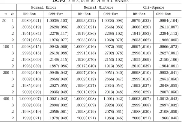
Table 5 presents the results based on DGP3, the FE-SDPD model with SL and STL, where H = H-I, T = 3 and SNR = 3. As the main focus of this set of Monte Carlo experiments is to compare the proposed robust M-estimator with the GMM estimator of Kuersteiner and Prucha (2018), we only report the empirical means and sds for these two estimators.9 The results show clear convergence patterns of both estimators: as sample size grows both estima-tors become less biased and less variable. The robust M-estimator has a smaller bias than the GMM estimator for all sample sizes and all three different error distributions. The empirical sds show that the robust M-estimator is much more efficient than the GMM estimator.
5. Empirical Application: Sovereign Risk Spillover
This section presents an empirical application of the proposed M-estimator for the FE-SDPD model under small T and unknown heteroskedasticity. We investigate international spillover of the sovereign bond spreads of 51 countries from 2007 to 2012, and we find that it is important to allow for heteroskedasticity in the estimation.
The increasing economic and financial integration worldwide has led to a continuous discussion of global transmission of risk in the past two decades, especially after the European sovereign debt crisis from 2010 to 2012. Many studies have applied the spatial econometrics frameworks to analyse risk spillovers. Sald´ıas (2013) uses a spatial error model to identify sector risk determinants. Favero (2013) uses a GVAR approach that incorporates the space-time lag to model the government bond spreads in the Euro area. Keiler and Eder (2015) use a spatial lag model to model the credit default swap (CDS) spreads of financial institutions, whereas Tonzer (2015) uses a spatial lag model to analyse the banking sector risk. Blasques et al. (2016) model sovereign CDS spreads using spatial Durbin panel data model with time-varying spatial dependence parameter. Debarsy et al. (2018) use a spatial dynamic panel data model to measure sovereign risk spillover considering different channels of risk transmission.
8Halleck Vega and Elhorst (2015) advocate spatial Durbin models. There can be issues of identification
and overfitting with Durbin models, especially when all spatial terms are included in the model and the same spatial weight matrix is used for all. See Elhorst (2012) and Lee and Yu (2016) for more details.
9
To implement the GMM in Kuersteiner and Prucha (2018) we use the code provided by the authors at:
All of these works are under the assumption that disturbances are homoskedastic. However, as different financial sectors vary greatly in size and depth, different countries vary greatly in so many aspects such as population, location, completeness of financial market, bureaucratic quality, government stability, openness to trade, and other social-economical characteristics, it is natural to think that we should allow the innovations to be heteroskedastic.
Our data covers 51 countries, including both advanced and emerging markets over six years from 2007 to 2012. The list of countries included in our analysis is presented in Ta-ble E1. Bond yield spread, credit default swap and credit ratings are three commonly used measures of sovereign risk in the literature. We follow the main body of the literature to measure the sovereign risk by sovereign bond yields spreads. For advanced economies, the spread is computed as the difference between the 10-year bond yields on the secondary market and the 10-year US treasury bond yield. We obtain the data from Datastream. For emerg-ing markets, we use Emergemerg-ing Market Bond Index Global (EMBIG) obtained from Global Economic Monitor of the World Bank database to measure the spreads in order to have a consistent measure for both advanced and emerging economies as in Beirne and Frazscher (2013) and Debarsy et al. (2018). In line with the literature, the set of exogenous explanatory variables we use contains debt-to-GDP ratio, deficit-to-GDP ratio, current account balance (CA) to GDP ratio, real GDP growth rate, inflation (CPI), real effective exchange rate and the volatility index (VIX). The first five variables control the macroeconomic and financial fundamentals of each country and the last variable controls the general market conditions. The data for these variables are collected from IMF World Economic Outlook (WEO). We use yearly data because it is the original frequency for most of the variables we consider. The original frequencies are daily for VIX and the bond yield spread, and monthly for real effective exchange rate. We use the average values over a year for those variables.
Table E1. List of Countries
Argentina Australia Austria Belgium Brazil Bulgaria Canada
Chile China Colombia Czech Republic Denmark Ecuador Egypt
Finland France Germany Ghana Greece Hungary Indonesia
Ireland Italy Jamaica Japan Kazakhstan Korea Malaysia
Mexico Netherlands New Zealand Norway Pakistan Panama Peru
Philippines Poland Portugal Russia Singapore South Africa Spain
Sweden Switzerland Tunisia Turkey Ukraine United Kingdom Uruguay
Venezuela Vietnam
We fit the data to the general model (2.1) and several sub-models, and report the results corresponding to the following two models that best fit the data: the SDPD model withSL andSTL:yt=ρyt−1+λ1W yt+λ2W yt−1+Xtβ+Zγ+µ+vt, and the SDPD model withSE
only: yt=ρyt−1+Xtβ+Zγ+µ+ut, ut=λ3W3ut+vt.
Both specifications are in fact widely used in empirical studies. In both models, yt is
observed time varying exogenous variables, Z is an n×kz matrix containing the observed
time invariant variables,µis ann×1 vector of unobserved country-specific fixed effects, and the elements{vit}ofvtare assumed to be iidacross time butinidacross country with mean
zero and varianceσ2vhi. We consider three different weight matrices to investigate three risk
transmission channels. The first weight matrix, Wtrade, represents the real linkage between
economies, and it is constructed using bilateral trade flow to measure the connectivity between countries. The (i, j) element ofWtrade,tisWijt= GDPMijtit+GDP+Xijtjt, whereMijtis the total import
of country i from country j in year t represented in US Dollars, Xijt is the total export of
country i to country j in year t, GDPit is the nominal gross domestic product for country i in year t and Wtrade is the time average of Wtrade,t. The data for bilateral trade volume
is collected from the World Integrated Trade Solution (WITS) database, and the data for GDP is available in the WEO database. The second and third weight matrices,Wdeficit and Wdebt, represent the information linkage between economies, and they are constructed using
similarities in debt or deficit level to measure the connectivity of government risk. Elements of these two weight matrices are the time average ofWijt= |Ait−A1jt|+1, whereAit is
debt-to-GDP ratio or deficit-to-debt-to-GDP ratio of countryiat time t. See Favero (2013) and Debarsy et al. (2018) for more discussions on the transmission channels.
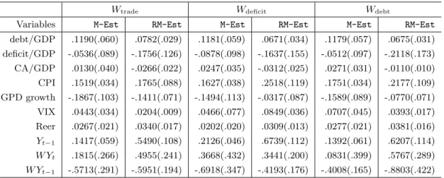
Table E2. Estimation Results of SDPD Model with SL and STL
Wtrade Wdeficit Wdebt
Variables M-Est RM-Est M-Est RM-Est M-Est RM-Est
debt/GDP .1190(.060) .0782(.029) .1181(.059) .0671(.034) .1179(.057) .0675(.031) deficit/GDP -.0536(.089) -.1756(.126) -.0878(.098) -.1637(.155) -.0512(.097) -.2118(.173) CA/GDP .0130(.040) -.0266(.022) .0247(.035) -.0312(.025) .0271(.031) -.0110(.010) CPI .1519(.034) .1765(.088) .1627(.038) .2518(.119) .1751(.034) .2177(.109) GPD growth -.1867(.103) -.1411(.071) -.1494(.113) -.0317(.087) -.1589(.089) -.0770(.071) VIX .0443(.034) .0204(.009) .0466(.077) .0849(.036) .0707(.045) .0393(.017) Reer .0267(.021) .0340(.017) .0202(.020) .0309(.013) .0277(.021) .0381(.016) Yt−1 .1417(.059) .5490(.108) .2126(.046) .6739(.112) .1392(.061) .6207(.114) W Yt .1815(.266) .4955(.241) .3668(.432) .3441(.200) .0831(.399) .5767(.289) W Yt−1 -.5713(.291) -.5951(.194) -.6918(.347) -.4193(.176) -.4008(.165) -.8803(.422)
Table E2 shows the estimation results when the data is fit toSL-STLmodel. We compare the results from the M-estimation of Yang (2018) and the proposed robust M-estimation in this paper under all three weight matrices. Under the robust M-estimation, the signs for all parameters are as expected and the parameter estimates for debt/GDP, CPI, VIX and real effective exchange rate are significant regardless of which weight matrix is used. The results are in line with the previous studies. Under the M-estimation, the sign of parameter estimate for CA/GDP is not as expected although insignificant, and only the parameters of debt/GDP and CPI are significant. The parameter of time-lag variable is estimated to be positive and significant under both methods but the magnitudes are much larger for robust
M-estimates. Under the robust M-estimation, the parameter of spatial-lag variable is estimated to be positive and significant whenWtrade andWdebtare used and insignificant whenWdeficit
is used. Under the M-estimation, the parameter estimates for spatial-lag variable are positive but insignificant under all three weight matrices and the magnitudes are smaller than those of the robust M-estimates. Parameter estimates for space-time lag variable are negative and significant for all weight matrices under the robust M-estimation, whereas it is insignificant whenWdeficit is used under the M-estimation.
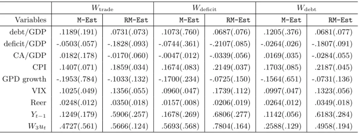
Table E3 shows the estimation results when the data is fit toSEmodel. First, we observe that the signs of parameter estimates for all variables stay the same and the magnitudes remain similar for both methods. The parameter estimate of debt/GDP becomes insignificant whereas the parameter estimate of deficit/GDP becomes significant under the robust M-estimation for all weight matrices. Under the M-M-estimation, both debt/GDP and deficit/GDP are insignificant in this model. The results for other variables are similar to those from STL model. The spatial error parameter and the dynamic parameter are estimated to be positive and significant by the robust M-estimation, but insignificant under the M-estimation.
Table E3. Estimation Results of SDPD Model with SE
Wtrade Wdeficit Wdebt
Variables M-Est RM-Est M-Est RM-Est M-Est RM-Est
debt/GDP .1189(.191) .0731(.073) .1073(.760) .0687(.076) .1205(.376) .0681(.077) deficit/GDP -.0503(.057) -.1828(.093) -.0744(.361) -.2107(.085) -.0264(.026) -.1807(.091) CA/GDP .0182(.178) -.0170(.060) -.0047(.012) -.0339(.056) .0169(.035) -.0284(.055) CPI .1407(.071) .1859(.034) .1674(.083) .2149(.037) .1703(.085) .2187(.045) GPD growth -.1953(.784) -.1033(.132) -.1700(.234) -.0725(.150) -.1564(.651) -.0731(.136) VIX .1025(.049) .1356(.055) .0960(.047) .1739(.112) .0997(.047) .1323(.056) Reer .0248(.012) .0350(.018) .0157(.008) .0206(.019) .0264(.012) .0349(.018) Yt−1 .1249(.179) .5906(.257) .1678(.269) .6806(.277) .1142(.056) .6183(.284) W3ut .4727(.561) .5666(.124) .5693(.568) .7804(.164) .2588(.129) .4958(.194)
6. Conclusion and Discussion
This paper considers the M-estimation and inference methods for the SDPD models with fixed effects and unknown heteroskedasticity, based on short panels. The estimation method extends the idea of Yang (2018) to allow for unknown heteroskedasticity by using modifi-cation terms that are quadratic in disturbances. The modified quasi-score function gives unbiased estimating equations. The statistical inferences are based on the outer-product-of-martingale-differences(OPMD) method proposed by Yang (2018). The asymptotic properties of the M-estimators and the estimators of VC matrix are studied. Monte Carlo experiments show that both the robust M-estimators and the estimators of standard errors perform very well and that ignoring the heteroskedasticity would cause significant bias. We apply our
methods to investigate the international government risk spillover through both real linkage and information channels. The results show that allowing for heteroskedastic disturbances can be important. The proposed methods, therefore, provide a useful set of econometrics tools for applied researchers.
We have studied the case where the disturbances are heteroskedastic across individuals. It would be interesting to further extend our method to allow for heteroskedasticity in both individual and time, and for serial correlation. It would also be interesting to extend our method to allow for endogenous regressors, interactive fixed effects, time varying weight matrices and time varying spatial parameters. These models would be more challenging and are beyond the scope of this paper, and will be studied in future works.
Appendix A: Some Basic Lemmas
The following lemmas are essential for the proofs of the main results in this paper, where Lemmas A.4 and A.5 extend those of Yang(2018) by allowingvit to be inid acrossi.
Lemma A.1. (Kelejian and Prucha, 1999; Lee, 2002): Let {An} and {Bn} be two
se-quences of n×nmatrices that are uniformly bounded in both row and column sums. Let Cn
be a sequence of conformable matrices whose elements are uniformlyO(ι−n1). Then (i) the sequence{AnBn} are uniformly bounded in both row and column sums,
(ii) the elements of An are uniformly bounded and tr(An) =O(n), and
(iii) the elements of AnCn and CnAn are uniformly O(ι−n1).
Lemma A.2. (Lee, 2004, p.1918): For W1 and B1 defined in Section 2, if kW1k and
kB10−1kare uniformly bounded, wherek · k is a matrix norm, thenkB1−1kis uniformly bounded in a neighborhood ofλ10.
Lemma A.3. (Lee, 2004, p.1918): Let Xn be an n×p matrix. If the elements Xn are
uniformly bounded andlimn→∞ n1Xn0Xnexists and is nonsingular, thenPn=Xn(Xn0Xn)−1Xn0
andMn=In−Pn are uniformly bounded in both row and column sums.
Lemma A.4. (Yang, 2018) Let{An} be a sequence ofn×n matrices that are uniformly
bounded in either row or column sums. Suppose that the elements an,ij of An are O(ι−1)
uniformly in alliand j. Let vn be a random n-vector of inid elements satisfying Assumption
B, and bn a constant n-vector of elements of uniform order O(ι−1/2). Then
(i) E(vn0Anvn) =O(ιnn), (ii) Var(v0nAnvn) =O(ιnn),
(iii) Var(vn0Anvn+b0nvn) =O(ιnn), (iv)vn0Anvn=Op(ιnn),
(v) vn0Anvn−E(vn0Anvn) =Op((ιnn) 1 2), (vi)v0 nAnbn=Op((ιnn) 1 2),
and (vii), the results(iii)and (vi) remain valid if bn is a randomn-vector independent ofvn
such that{E(b2ni)} are of uniform order O(ι−n1).
Lemma A.5. (Yang, 2018, Central Limit Theorem for bilinear quadratic forms): Let {Φn} be a sequence of n×n matrices with row and column sums uniformly bounded, and
elements of uniform order O(ι−n1). Let vn be a random n-vector satisfying Assumption B.
Let bn ={bni} be an n×1 random vector, independent of vn, such that (i) {E(b2ni)} are of
uniform order O(ι−1
n ), (ii) supiE|bni|2+0 <∞,(iii) ιnnPni=1[φn,ii(bni−Ebni)] =op(1) where
{φn,ii} are the diagonal elements of Φn, and (iv) ιnnPni=1[b2ni−E(b2ni)] = op(1). Let Hn=
diag(hn1, . . . , hnn). Define the bilinear-quadratic form:
Qn=b0nvn+vn0Φnvn−σ2vtr(ΦnHn),
and let σ2
Qn be the variance of Qn. If limn→∞ι
1+2/0
n /n= 0 and {ιnnσQ2n} are bounded away from zero, thenQn/σQn
d
Appendix B: Proofs of Theoretical Results
Proof of Lemma 3.1: By (2.3), ∆yt=B0∆yt−1+B10−1∆Xt+B10−1B
−1
30∆vt, t= 2, . . . , T,
backward substitution leads to E(∆yt∆v0t) =−σv02 (B0−2In)B−101B
−1 30H,t= 2, . . . , T, E(∆yt∆v0t+1) = −σ2 v0B −1 10B −1
30H,t= 1, . . . , T −1, and E(∆yt∆vs0) = 0 ifs≥t+ 2; and
E(∆yt∆vs0) =B0E(∆yt−1∆vs0) =B20E(∆yt−2∆vs0) = · · ·
=B0t−sE(∆ys∆vs0) +Bt0−s−1B −1 10B −1 30E(∆vs+1∆vs0) =B0t−s+1E(∆ys−1∆vs0) +Bt −s 0 B −1 10B −1 30E(∆vs∆vs0) +Bt −s−1 0 B −1 10B −1 30E(∆vs+1∆vs0) =B0t−s+1B10−1B30−1E(∆vs−1∆v0s) +Bt −s 0 B −1 10B −1 30E(∆vs∆v 0 s) +Bt −s−1 0 B −1 10B −1 30E(∆vs+1∆v 0 s) =−Bt0−s+1B10−1B30−1σv02 H+ 2B0t−sB10−1B30−1σv02 H − B0t−s−1B10−1B30−1σv02 H =−σv02 Bt0−s−1(B0−In)2B10−1B −1 30H,
ifs≤t−1. Summarizing above, we obtain the results of Lemma (3.1).
Proofs of the theorems need the following matrix results: (i) the eigenvalues of a projection matrix are either 0 or 1; (ii) the eigenvalues of a positive definite (p.d.) matrix are strictly positive; (iii) γmin(A)tr(B)≤tr(AB)≤γmax(A)tr(B) for symmetric matrix A and positive
semidefinite (p.s.d.) matrixB; (iv)γmax(A+B)≤γmax(A)+γmax(B) for symmetric matrices AandB; and (v)γmax(AB)≤γmax(A)γmax(B) for p.s.d. matricesAandB(Bernstein, 2009).
Proof of Theorem 3.1: Use ∆ˆu(δ) defined below (2.6) and ∆¯u(δ) defined below (3.23). Let B∗r = Ω−12Br, where Ω
1
2 is the square-root matrix of Ω. We can write ∆ˆu∗(δ) =
Ω−12∆ˆu(δ) = M(B∗
1∆Y −B∗2∆Y−1) and ∆¯u∗(δ) = Ω− 1
2∆¯u(δ) = M(B∗
1∆Y −B∗2∆Y−1) +
P[B∗1(∆Y−E(∆Y))−B2∗(∆Y−1−E(∆Y−1))], whereP= Ω− 1
2∆X(∆X0Ω−1∆X)−1∆X0Ω− 1 2,
andM=In(T−1)−P. By (3.14) and (3.23), we have
ˆ
σv,2M(δ) = n(T1−1)(B∗1∆Y −B∗2∆Y−1)0M(B∗1∆Y −B∗2∆Y−1),
¯
σv,2M(δ) = n(T1−1)tr[Var(B∗1∆Y −B∗2∆Y−1)]
+n(T1−1)(B∗1E∆Y −B∗2E∆Y−1)0M(B∗1E∆Y −B∗2E∆Y−1).
The second term in ¯σ2v,M(δ) is nonnegative uniformly inδ∈∆ asMis p.s.d. For the first term, by the definition of the matrix C, Assumption E(iv) and the assumption (ii) given in the theorem, n(T1−1)tr[Ω−1Var(B1∆Y−B2∆Y−1)]≥ n(T1−1)γmin(C−1)γmin(B30B3)tr[Var(B1∆Y−
B2∆Y−1)] > c >0, uniformly in δ ∈ ∆, implying infδ∈∆σ¯2v,M(δ) > c >0. It is easy to show
that supδ∈∆|σˆv,2M(δ)−σ¯v,2M(δ)|= op(1). Therefore, we can drop ˆσv,2M(δ) in the concentrated
AQS function (3.15) and ¯σv,2M(δ) in its population counter part (3.24) and write:
SSTLE∗c (δ)−S¯STLE∗c (δ) = ∆ˆu(δ)0Ω−1∆Y −1−E[∆¯u(δ)0Ω−1∆Y−1] + ∆ˆu0(δ)Eρ∆ˆu(δ)−E[∆¯u0(δ)Eρ∆¯u(δ)], ∆ˆu(δ)0Ω−1W1∆Y −E[∆¯u(δ)0Ω−1W1∆Y] + ∆ˆu(δ)0Eλ1∆ˆu(δ)−E[∆¯u(δ) 0E λ1∆¯u(δ)], ∆ˆu(δ)0Ω−1W2∆Y −1−E[∆¯u(δ)0Ω−1W2∆Y−1] + ∆ˆu(δ)0Eλ2∆ˆu(δ)−E[∆¯u(δ) 0E λ2∆¯u(δ)] ∆ˆu(δ)0Υ∆ˆu(δ)−E[∆¯u(δ)0Υ∆¯u(δ)],

![Table 1a. Empirical Mean(sd)[rse] ∗ of CQMLE, M-estimator, and Robust M-estimator, DGP1, T = 3, m = 10, H=H-I, SNR=1 ;](https://thumb-us.123doks.com/thumbv2/123dok_us/9470938.2821986/34.1262.134.1110.151.732/table-empirical-mean-cqmle-estimator-robust-estimator-dgp.webp)