Preconditioned optimization algorithms solving the problem of the non unitary joint block diagonalization: application to blind separation of convolutive mixtures

HAL Id: hal-01785915

https://hal-amu.archives-ouvertes.fr/hal-01785915

Submitted on 18 May 2018

HAL

is a multi-disciplinary open access

archive for the deposit and dissemination of

sci-entific research documents, whether they are

pub-lished or not. The documents may come from

teaching and research institutions in France or

abroad, or from public or private research centers.

L’archive ouverte pluridisciplinaire

HAL, est

destinée au dépôt et à la diffusion de documents

scientifiques de niveau recherche, publiés ou non,

émanant des établissements d’enseignement et de

recherche français ou étrangers, des laboratoires

publics ou privés.

Preconditioned optimization algorithms solving the

problem of the non unitary joint block diagonalization:

application to blind separation of convolutive mixtures

Omar Cherrak, Hicham Ghennioui, Nadège Thirion-Moreau, El Houssein

Abarkan

To cite this version:

Omar Cherrak, Hicham Ghennioui, Nadège Thirion-Moreau, El Houssein Abarkan. Preconditioned

optimization algorithms solving the problem of the non unitary joint block diagonalization: application

to blind separation of convolutive mixtures. Multidimensional Systems and Signal Processing, Springer

Verlag, 2017. �hal-01785915�

Preconditioned

optimization

algorithms

solving

the

problem

of

the

non

unitary

joint

block

diagonalization:

application

to

blind

separation

of

convolutive

mixtures

OmarCherrak1,2,3 ·HichamGhennioui1 · NadègeThirion-Moreau2,3 ·ElHossainAbarkan1

Abstract This article addresses the problem of the Non Unitary Joint Block

Diagonalization (NU −JBD) of a given set of complex matrices for the blind separation of convolutive mixtures of sources. We propose new different iterative optimization schemes based onConjugate Gradient, Preconditioned Conjugate Gradient,Levenberg–Marquardt and Quasi-Newton methods. We perform also a study to determine which of these algorithms offer the best compromise between efficiency and convergence speed in the studied context. To be able to derive all these algorithms, a preconditioner has to be computed which requires either the calculation of the complex Hessian matrices or the use ofan approximationto theseHessianmatrices. Furthermore,the optimal stepsizeis also computed algebraically to speed up the convergence of these algorithms. Computer simulations are provided in order to illustrate the behavior of the different algorithms in various contexts: when exactly block-diagonal matrices are considered but also when these matrices are progressively perturbed by an additive Gaussian noise. Finally, it is shown that these algorithms enable solving the blind separation of the convolutive mixtures of sources problem.

Keywords Joint block diagonalization ·Blind source separation ·Preconditioning ·

Complex Hessian matrices ·Convolutive mixtures ·Spatial quadratic time-frequency

B

1 _{Faculté des Sciences et Techniques de Fès, LSSC, Université Sidi Mohamed Ben Abdellah,}

Route Immouzzer, B.P. 2202, Fès, Maroc

2 _{CNRS, ENSAM, LSIS, UMR 7296, Aix-Marseille Université, 13397 Marseille, France} 3 _{CNRS, LSIS, UMR 7296, Université de Toulon, 83957 La Garde, France}

MathematicsSubjectClassification 60G35 ·65K10 ·15A69 ·65F08 ·65F10

1

Introduction

With the use of more antennas equipped with more receivers, the volume of available data iscontinuallyincreasingandadvancedsignalprocessingtechniquesareoftenrequiredtobe able to extract relevant information from this huge amount of data. The problem of the joint decomposition of matrices (or tensors) sets can come within this framework, that is why it has gained a growing attention from the signal processing scientific community over the recent years. Whatever the considered field of application (astronomy, geophysics, remote sensing, biomedical, etc.), algorithms addressing the aforementioned problem are of interest if the problemathandcanfinallybeformulatedasaproblemofArrayProcessingand Direction-Of-Arrival estimation, Blind Source Separation (BSS), blind multidimensional deconvolution or even data mining or analysis.

Because traditionally a pre-whitening stage was used, one of first problem to have been considered was the so-called Joint Diagonalization (JD)of a given matrix set under the uni-taryconstraint.Itledtothenowadayswell-knownJADE(JointApproximateDiagonalization of Eigenmatrices) CardosoandSouloumiac1993 and SOBI (Second Order Blind Identifi-cation) Belouchranietal.1997 algorithms. The following works have addressed either the problem of the JD of tensors (Comon1994; Moreau 2001) or the problem of the JD of matrix sets, discarding the unitary constraint (ChabrielandBarrère2012; Maurandietal. 2013; Souloumiac2009; Yeredor2002). A fairly exhaustive overview of all the suggested approachesisavailableinChabrieletal.2014.Thisfirstparticulartypeofmatrix decom-position proves useful to solve two kinds of problems i) those of sources localization and direction finding and ii) those of blind separation of instantaneous mixtures of sources.

At the same time, people have started to consider a second type of matrix decompositions -namely joint zero-diagonalization (JZD) -, since it is not uncommon to encounter this problem in different field of applications such as blind source separation (and more specifically spatial quadratic time-frequency domain methods (Belouchranietal.2001; Belouchranietal.2013)), telecommunications ChabrielandBarrère2011 and cryptography Walgateetal.2000. The first proposed algorithms operated under the unitary constraint Belouchranietal.2001, since once again, they were applied after a classical pre-whitening stage. But such a preliminary pre-whitening stage establishes a bound with regard to the best performances in the context ofBSSthatiswhytheunitaryconstraintwassoondiscarded,leadingtoseveralsolutions among which are (Fadailietal.2007; Chabrieletal.2008).

Recently, a more general problem has been addressed: that of the joint decomposition of a combination of given sets of complex matrices that can follow potentially different decompositions (for example when noncircular complex valued signals are considered and when people want to exploit additional statistical information by using both Hermitian and complexsymmetricmatricessimultaneously)(MoreauandAdali2013;TraininiandMoreau 2014; Zengetal.2009). Such issues can arise in various signal processing problems, among which are blind identification, separation or multidimensional deconvolution.

In this article, we focus on a fourth type of matrix decompositions, namely the Joint Block-Diagonalization (JBD). It is a rather general problem since the aforementioned JD problemisaspecialcaseofthisone,butitcouldbeseenasapartofthethirdproblemeven if - to our knowledge - only JD problems have been considered in that context up to this point. In such a decomposition, the matrices under consideration assume a specific algebraic structure,

being block diagonal matricesi.e.they are block matrices whose diagonal blocks are square matrices of any (possibly even) size while their off-diagonal blocks are all null. First, this problem was addressed considering positive definite and hermitian block-diagonal matrices and unitary joint-block diagonalizers. Jacobi like algorithms were suggested (Belouchrani et al. 1997;De Lathauwer et al. 2002). Then, different alternative methods achieving the same task but for a non unitary joint-block diagonaliser have been proposed (Cherrak et al. 2013b;Ghennioui et al. 2007;Ghennioui et al. 2010;Ghennioui et al. 2007b;Lahat et al. 2012a;Nion 2011;Tichavsky and Koldovsky 2012;Xu et al. 2010; (Zhang et al.(2016); Zhang and Zhang(2016) for video event recognition and object recognition)).

In this article, our goal is to investigate the impact/interest of the preconditioning process in theJBDalgorithms to be able to determine which method offers the best compromise between efficiency and convergence speed in the studied context (BSSand blind multidimensional deconvolution). But, first, to be able to derive the different algorithms, the preconditioner has to be determined. It is the reason why, we start with the theoretical calculation of the complex Hessian matrices. Then the different optimization algorithms can be derived and the optimal stepsize can be calculated. Computer simulations are provided in order to illustrate the behavior of the different algorithms in various contexts: when exactly block-diagonal matrices are considered but also when these matrices are progressively perturbed by an additive Gaussian noise. Finally, we show how these algorithms find applications in blind separation of a convolutive mixture of deterministic or random source signals, based on the use of Spatial Quadratic Time Frequency Spectra (SQTFS) or Spatial Quadratic Time Frequency Distributions (SQTFD).

This article is organized as follows: the general problem ofNU−JBDand the principle of preconditioning are reminded in Sect.2. In the Sect.3, we introduce the algebraic calculations of the Hessian matrices leading to the proposed possibly preconditionedNU−JBD algo-rithms. In Sect.4, we show the different classical deterministic iterative optimization schemes considered and we introduce the calculation of the optimal step-size. Computer simulations are provided in Sect.5in order to illustrate the behavior of the resulting preconditioned JBD(and possiblyJD) algorithms. To that aim, the different algorithms are compared in various contexts comparing them with “state-of the-art approaches”. The Sect.6enhance the usefulness of these algorithms through one of their possible applications, namely the blind separation of Finite Impulse Response (FIR) convolutive mixtures of non-stationary sources. Computer simulations are performed to illustrate the good performance of the suggested BSSmethods. Finally in Sect.7, a conclusion is drawn.

2 Problem statement and some recalls about optimization

2.1 The non unitary joint block-diagonalization problem and its assumptions

We recall that the problem of the non unitary joint block-diagonalization is stated in the following wayGhennioui et al. 2007. Provided that we have a setMofNmsquare matrices

Mi ∈CM×M, for alli ∈ {1, . . . ,Nm}that all admit the following decomposition:

Mi =ADiAH, (1)

where(·)H stands for the transpose conjugate (or Hermitian) operator and theNmsquare

Di= ⎛ ⎜ ⎜ ⎜ ⎜ ⎝ Di,11 012 . . . 01r 021 Di,22 ... ... ... ... ... 0r−1r 0r1 . . . 0rr−1 Di,rr ⎞ ⎟ ⎟ ⎟ ⎟ ⎠, (2)

withrthe number of considered blocks (r∈N∗),Di,j j,i ∈ {1, . . . ,Nm}, j ∈ {1, . . . ,r}

arenj×njsquare matrices so thatn1+ · · · +nr =N where0i jdenotes the(ni×nj)null

matrix.

Ais aM×N (M≥ N) full rank matrix whileA†_{is a pseudo-inverse ofA(or}

Moore-Penrose generalized matrix inverse). It is aN×Mmatrix denoted byB(B=A†). The set of theNmsquare matricesDi ∈CN×Nis denoted byD. The block sizesnjfor allj=1, . . . ,r

are assumed known. In the context of blind source separation,Ais known as the mixing matrix whereasBis called the separating matrix,N is the number of sources whileMis the number of sensors. ManyBSSmethods go through a joint matrix decomposition stage in order to estimate either the mixing matrix or the separating matrix even if other approaches have been considered too (direct or deflation methods for example). Moreover, this joint matrix decomposition problem often brings us back to a joint diagonalisation (resp. joint block diagonalisation) problem when instantaneous (resp. convolutive) mixtures of sources are considered. An unitary constraint on the matricesAorBis the result of a preprocessing stage called spatial whitening of the observations. But studies have proven that this step establishes a bound with regard to the best reachable performances in the context ofBSS. That is why recently, there has been a strong interest in methods discarding this constraint.

The general NU−JBD problem consists of estimating the matrix A and the block-diagonal matrices setD from only the matrix set M. It was shown inGhennioui et al. 2010, a standard way consists of minimizing the following quadratic objective function:

C(2) JBD(B,{Di})= Nm i=1 OffBdiag_(n){BMiBH}2F def =CJBD(B), (3)

where · Fstands for the Frobenius norm and the matrix operatorOffBdiag(n){·}can be defined as (Ghennioui et al. 2010):

OffBdiag_(n){M} =M−Bdiag_(n){M} = ⎛ ⎜ ⎜ ⎜ ⎜ ⎝ 011 M12 . . . M1r M21 ... ... ... ... ... ... ... Mr1 Mr2 . . . 0rr ⎞ ⎟ ⎟ ⎟ ⎟ ⎠, (4) where Bdiag_(n){M} = ⎛ ⎜ ⎜ ⎜ ⎜ ⎝ M11 012 . . . 01r 021 ... ... ... ... ... ... ... 0r1 0r2 . . . Mrr ⎞ ⎟ ⎟ ⎟ ⎟ ⎠. (5)

2.2Somerecallsaboutoptimizationandpreconditioning

In the literature, one can find many unconstrained optimization methods and some of them, namely gradient-descent, steepest descent, relative gradient and conjugate gradient methods

have already been studied and applied in this specific context ofJBD(Ghennioui et al. 2010; Nion 2011). They are known as first-order methods since they only depend on the gradient of the cost function and not on its second derivatives (i.e.the Hessian matrix denoted here byH_•. Notice that in the next section we will clarify this notation). To our knowledge, very few, if any, studies have been led on preconditioned optimization methods in such a framework. Yet, when one is designing an algorithm for a specific application, many conflicting requirements have to be taken into account (convergence rate (as few iterations as possible), computation time per iteration (as few floating point operations as possible), stability, sensitivity to numerical errors, robustness versus noise and/or model errors, problems of initialization, storage requirements, potential parallelization, ease of implementation, real time implementation, just to name a few), and at the end, for one given application, one must choose the algorithm which offers the best compromise between all those requirements. That is why we have chosen, here, to look specifically at preconditioned optimization methods to determine whether they are interesting or not for joint block diagonalization problems.

The main purposes for which preconditioning is generally used, are:

– to further accelerate the convergence since gradient-descent or steepest descent algo-rithms are well known for their sometimes slow convergence,

– to increase stability and robustness versus noise or model errors,

– to cope with the fact that variables have wildly different magnitudes (since the most simple form of preconditioning is a scaling of the variables (thanks to a diagonal preconditioner) with well chosen coefficients),

– to cope with the fact that the cost function can rapidly change in some directions and slowly in other ones,

– to be able to tackle ill-posed problems,

– to ensure certain constraints such as non-negativity (see for example the nonnegative matrix factorization algorithm (NMF) based on multiplicative updates suggested by Lee and SeungLee and Seung 2000bwhich can be interpreted as a preconditioned gradient algorithm).

Sometimes the preconditioning process just speed up the convergence, but there also exist some difficult cases which cannot be solved without good preconditioning. That is why several works have addressed the problem of the design of effective preconditioners. First, the preconditioning has been used in direct methods and, latter this concept has been extended to the case of iterative processes (Chebyschev acceleration) in (Evans 1968;Turing 1948). The key issue remains obviously the choice of the preconditioner denoted byP. In the literature, one can find many works on different types of preconditioners, among which are the Jacobi and Gauss-Seidel preconditionersWestlake 1968. The first one consists of using the diagonal of the desired matrix while the second one consists of decomposing the preconditioner matrix into a lower triangular matrix, a diagonal matrix, and an upper triangular matrix. Yet, for non-symmetric problems, such preconditioners are limited in their effectiveness and robustness Axelsson 1985.

The analysis of the convergence rate of the proposed preconditioned gradient-descent method provides a substantial help in the choice ofPand directions to follow. If the cost function is twice differentiable in the neighborhood of a local minimizer,i.e.with Hessian matrixH_• def= ∇_B2CJBD

def

= ∂2CJBD_∂B∂B(B,B∗ ∗) then the fastest convergence is obtained when the

preconditionerPminimizes the condition number, namelyκ, of the productPH_•. The con-dition number stands for the ratio of the largest singular value ofPH•divided by the smallest singular value of this matrixi.e.κ def= λmax(PH•)

pre-conditioner would beP=(H_•)−1so thatPH_• =Isince the identity matrixIpossesses the minimal (unity) condition number. But since it is not always easy to calculate or to compute (H_•)−1_{(especially whenNorMbecome large in our case), it remains interesting to develop}

preconditioners that approximate(H•)−1and that are cheaper to construct and to apply (Chen 2005a;Benzi 2002).

To be able to design a suitable preconditioning matrixPin the context ofJBD, we will start with the calculation of the four exact complex Hessian matrices. Then, we will be able to derive several new preconditioned algorithms among which is a preconditioned Conjugate Gradient algorithm. The conjugate gradient method is an iterative optimization method which has become really popular in nonlinear optimization (Hager and Zhang 2006;Paatero 1999) and its efficiency may be improved by a proper choice of the preconditioning matrixAxelsson 1985.

3 New preconditioned joint block-diagonalization algorithms

To estimate the complex matrixB∈CN×M_{, the cost function given in (3) has to be minimized.}

To that aim, the differentialdCJBDofCJBDhas to be derived, involving the calculation of the

partial derivatives_∂∂_·of the objective functionCJBDwith respect toBandB∗(it is the reason

why, from now on, the objective function is denoted byCJBD(B,B∗)whereB∗stands for

the complex conjugate of the complex matrixB, except in 4.4). Then, the complex gradient matrix can be derived. In fact, theN×Mcomplex gradient matrix of our real-valued scalar cost function given in (3) denoted∇BCJBDhas been calculated inGhennioui et al. 2010and

found to be equal to: ∂CJBD(B,B∗) ∂B∗ = Nm i=1 OffBdiag_(n){BMiBH}BMiH+ OffBdiag_(n){BMiBH} H BMi . (6) Eventually, the second order differentiald2_C

JBDcan be calculated too in order to derive

the complex Hessian matrices. The complex matrixHis a square 2N M ×2N M matrix constituted of fourN M×N Msquare blocks which are the Hessian matrices:

H= HB,B∗ HB∗,B∗ H_B,B HB∗,B . (7)

To calculate the aforementioned matrixH, we follow the same path as inHjorungnes, A. 2011(details of this calculation can be found in the Appendix). In short, we have to derive the expression of the second-order complex differential ofCJBD(B,B∗)which is then written

as: d2CJBD(B,B∗)= dvecT(B∗)dvecT(B) A00A01 A10A11 dvec(B) dvec(B∗) . (8)

As shown inHjorungnes, A. 2011, the fourN M×N Mcomplex matricesA00,A01,A10

andA11involved in the above expression are linked to the Hessian matrices by:

HB,B∗C_JBD(B,B∗)= A00+A T 11 2 = HB∗,B CJBD(B,B∗) T , (9) HB∗,B∗ CJBD(B,B∗) = A01+AT01 2 , (10)

H_B,BCJBD(B,B∗)

= A10+AT10

2 . (11)

There are shown to be equal to (see the Appendix1for the detailed mathematic develop-ments): A00= MT_iBT⊗IN TT_BoffB∗M∗_i ⊗IN+ M∗_iBT⊗IN TT_BoffB∗MT_i ⊗IN +M_i∗⊗OffBdiag_(n){BMiBH} +MiT⊗OffBdiag(n){BMiHBH} =A∗11, (12) A10=KTN,M IN⊗MiBH TT_BoffB∗M∗_i ⊗IN +KT_N,M IN⊗MiHBH T_BoffT B∗M_iT⊗IN =A∗₀₁, (13)

where the operator⊗denotes the Kronecker product,KN,Mis a square commutation matrix

of sizeN M×N MandTBoff=IN2−T_Diag, is theN2×N2“transformation” matrix, with

TDiag =diag{vec(BDiag{1N})},1N is theN ×N matrix whose components are all ones,

diag{a}is a square diagonal matrix whose diagonal elements are the elements of the vector

a,IN2 = Diag{1_N2}is the N2×N2 identity matrix, andDiag{A}is the square diagonal matrix with the same diagonal elements asA.

One can check that the bigger complex matrixHdefined in (7) is hermitian and that two parts can be distinguished in this matrixH: its block-diagonal part and its off-block diagonal part.

According toShewchuk 1994b, it is advisable to consider only the diagonal (real part) of the Hessian matrixi.e.(9) and (12) to ensure a non increase of the cost function, and to easily obtain its inverse. TheN M×N Mpreconditioning matrix, denoted byP, that we suggest thus, reads: P=(H)−1, (14) H=DiagH_B,B∗C_JBD(B,B∗)=DiagHB∗,B CJBD(B,B∗) . (15)

Hence in the next sections, we can focus on the different possibly preconditioned algo-rithms that can be derived, and try to better assess their behavior in different contexts.

4 Classical deterministic iterative optimization schemes

To estimate the joint block diagonalizerB, the cost function given in (3) has to be minimized. To that aim different deterministic iterative optimization schemes can be considered. It means thatB has to be re-estimated at each iterationm, so from now on, it will be denoted by

B(m)_{. This matrix can also be stored in a vector b}(m)_{if thevec(·)operator is appliedi.e.}

b(m) _{= vecB}(m)_{. Depending on the considered optimization scheme,B}(m) _{for allm is}

updated according to one of the following adaptation rules. For example, when a classical steepest descent approach is considered (gradient approach if the step size is a fixed positive scalari.e.μ(m)=μfor allm),Bis updated at each iterationm(m=1,2, . . .) according to:

B(m+1)=B(m)−μ(m)∇BCJBD(B(m),B∗(m)), (16)

or equivalently,

b(m+1)=b(m)−μ(m)g_B(m∗), (17)

where∇BCJBD(B(m),B∗(m))is the gradient matrix given in (6) org(_Bm∗)is its vectorized form i.e.g(_Bm∗)=

DB∗(CJBD(B(m),B∗(m)))

T

size (the problem of its choice is treated in the Sect.4.4). This algorithm may converge slowly, that is why we are interested in preconditioned algorithms in order to speed up the convergence.

4.1 Preconditioned non linear conjugate gradient

To further accelerate convergence, conjugate gradient methods modify the search directions to ensure that they are approximately mutually conjugatei.e.orthogonal with respect to an inner product related to the Hessian of the cost function. Thus, when the preconditioned conjugate gradient algorithm is considered, the search direction,d, is given at the first iteration by:

d(1)= −P(1)g(_B1∗). (18)

Then,∀m=2, . . ., the following adaptation rule is used:

b(m+1)=b(m)+μ(m)d(m),

d(m+1)= −P(m+1)g_B(m∗+1)+β(m)d(m),

(19) where the expression of the preconditionerPis given in (14)-(15). It should be a positive-definite matrix, so non positive diagonal elements are prohibited: if it occurs, the algorithm is no more preconditioned (Pis then set to the identity matrixIN Mand we come back to the

classical non linear conjugate gradient algorithm). In exact line search method, we use the Polak-Ribière (βPR) formulaPolak 1997awhich is given by:

β(m+1)

PR =

(g(_Bm∗+1)−g(_Bm∗))HP(m+1)g_B(m∗+1)

(g(_Bm∗))HP(m)g_B(m∗)

. (20)

However, several expressions for β are classically used: the Fletcher-Reeves (βFR)

Shewchuk 1994band the Dai-Yuan (βDY)Yuan 1999. The resulting algorithm is denoted

byJBDPCGEH(EHstands for Exact Hessian).

4.2 Levenberg–Marquardt algorithm

When the Hessian matrixHtends to lose its positive-definiteness property through the itera-tions, and hence may fail to construct descent direcitera-tions, it is better to stabilize it using trust region techniques that modifyHby adding a multiple of the identity matrix. It is the principle of the Levenberg–Marquardt approachLuenberger 1969a:

b(m+1)=b(m)−μ(m) H(m)+αINM −1 g(_Bm∗), (21)

where α is a relaxation coefficient. We notice that by setting H = IN M in (21) (or by

considering that αis chosen high enough), the gradient algorithm

in (17) may be obtained. It can also be seen as a variant of the preconditioned conjugate gradient algorithm given in (19) where β=0 and where the preconditioner is not directly the inverse of the Hessian but is slightly modified. With regards to H, we can use either our solution given in (14)-(15). The resulting algorithm is denoted by

JBDLMEH(again EH stands for Exact Hessian).

4.3Quasi-Newtonalgorithm

In (21), by setting α=0 and considering that the preconditioner Pis a N M×N M calculation

adaptation rule. In this case, the algorithm is initialized using forP(1)(orH(1)), a symmetric,

N M×N Mpositive-definite matrix. The resulting algorithm is denoted byJBDQNEH (QN

standing for Quasi-Newton).

4.4 Choice of the step size: Enhanced Line Search or seek of the optimal step-size

It remains essential to find a good stepsizeμin the given search directiond(m) at each iterationm. This stepsizeμ(m)can be found in different ways: it can be fixed or decreased versus the iterations, or we can opt for a global search with Enhanced Line Search (ELS) or for an approximation by a line search method like backtrackingVandenberghe 2004(which is a locally optimal stepsize method).

This subsection is dedicated to the calculation of the optimal stepsize which is denoted byμopt. When the preconditioned conjugate gradient algorithm is considered for

exam-ple, it implies the algebraical calculation of the following quantity: CJBD(B(m+1)) =

CJBD

B(m)_−μD(m)_{, where D}(m) _{= unvecd}(m) _{or equivalently d}(m) _{= vecD}(m)

where the vectord(m)_{is given in (19) (operatorunvecenables to come back to a matrix). It is}

a 4th-degree polynomial whose expression is given by (to simplify the different expressions, the dependency upon the iterationmis omitted):

CJBD(B−μD)=a0+a1μ+a2μ2+a3μ3+a4μ4, (22)

where the five coefficientsa0,a1,a2,a3anda4are found equal to (see the Appendix1for

the details mathematic developments), a0= Nm i=1 trCH₀OffBdiag₍n){C0} , (23) a1= − Nm i=1 trC₁HOffBdiag_(n){C0} +C0HOffBdiag(n){C1} , (24) a2= Nm i=1

trCH₂OffBdiag_(n){C0} +C1HOffBdiag(n){C1} +C0HOffBdiag(n){C2}

, (25) a3= − Nm i=1 trC₂HOffBdiag₍n){C1} +C1HOffBdiag(n){C2} , (26) a4= Nm i=1 trCH₂OffBdiag_(n){C2} , (27) with C0=BMiBH, (28) C1=BMiDH+DMiBH, (29) C2=DMiDH. (30)

Then, the third order polynomial (31) corresponding to the derivative with respect toμof the 4th-degree polynomial given in (22) is calculated and its three roots are derived:

∂CJBD(B−μD)

∂μ =4a4μ3+3a3μ2+2a2μ+a1. (31)

Finally the optimal stepsize,μopt, corresponds to the root that leads to the smallest value

4.5 Algorithms proposed

The non-unitaryJBDproposed algorithms are summarized below:

Data:Nmsquare matricesM1,M2, . . . ,MNm, stopping criterion, step-sizeμ, max. number of iterationsNmax, number used for restartN0, relaxation coefficientα

Result: Estimation of the joint block diagonalizerB

initialize:B(0);D(0);m=0;

repeat

if(For(P)CGalgorithms only) m mod N0=0then

restart

else

Calculate optimal step-sizeμ(_optm)(root of (31) leading to the smallest value of (22)) Compute gradient matrix∇BCJBD(B(m+1), (B(m+1))∗)given in (6)

Compute exact Hessian matrixHgiven in (15)

JBD_CGalgorithm

Compute matrixB(m+1)thanks to (16) or (17)

JBDPCG_EHalgorithm

Compute exact preconditionerP(m+1)given in (14) Compute matrixB(m+1)thanks to (19)

Computeβ_PR(m)given by (20)

Compute the search directionD(m+1)thanks to (19)

JBDLMEHalgorithm

Compute matrixB(m+1)thanks to (21) Calculate the errore(m+1)= _N1

mCJBD(B (m+1)₎ ife(m+1)>e(m+1)then α=10α,e(m+1)=e(m) else α=10α end JBDQN_EHalgorithm

Compute exact preconditionerP(m+1)given in (14) Compute matrixB(m+1)thanks to (21) withα=0 m=m+1;

end

until((B(m+1)−B(m)2_F≤) or (m≥Nmax));

4.6 Complexity of algorithms

To compute the gradient matrix∇BCJBD

B(m+1), (B(m+1))∗whose expression is given in (6), the algorithmic complexityC1is:

M=N 4NmN M(M+N)+2N2Nm

MN 4NmN M2

M=N 8NmN3+2NmN2

To compute the preconditioning matrix according toP=DiagH_B,B∗(C_JBD(B,B∗)), the complexityC2is:

M=N 2Nm(M N(4M+3N)+M N4(M+N))

MN 8NmM2N+2NmM2N4

M=N 8NmN3+2N6

To update the search direction given in (19), using the Polak-Ribière formulaβ(m)given in (20), the complexity is:

M=N 2M3N3+4Nm(M N(4M+3N)+2M N4(M+N))+2N M(M+N)

MN 2M3N3+16NmM2N+8NmM2N4+2N M2

M=N 8N6+28NmN3+4N4

To compute the coefficientsa₀(m), . . . ,a₄(m) thanks to (23)–(27), and then to obtain the optimal step-sizeμ(_optm)by the search of the root of the polynomial given in (31) attaining the minimum in the polynomial given in (22), the complexity is:

M=N 24M N Nm(M+N)+9N2Nm(1+N)

MN 24M2N Nm

M=N 57N3Nm+9N2Nm

Finally, the total complexity for the different algorithms that we were able to derive is summed up in the following table:

Algorithm Algorithmic cost

JBDCG M=N 28NmN M(M+N)+11N2Nm+2N3M3+N M(M+N)+9N3Nm MN 11N2Nm+28NmN M2+2N3M3+9N3Nm+N M2 M=N 17NmN3+11N2Nm+2N6+2N3+48NmN3 JBDPCGEH M=N 2NmN M(20M+17N+5N 3_(M+N))+2N3_M3_+19N2_N m+9N3Nm MN 40NmN M2+10M2N4+2N3M3+19N2Nm+9N3Nm M=N 83NmN3+20N4+2N6+19N2Nm JBDLMEH M=N 2NmN M(18M+17N+N 3_(M+N))+11N2_N m+2N3M3+9N3Nm MN 36NmM2N+11N2Nm+2NmM2N4+2N3M3+9N3Nm M=N 88NmN3+4NmN6+2N6+2N2Nm JBDQNEH M=N 2NmN M(18M+17N)+11N 2_N m+2NmM N4(M+N)+9N3Nm MN 36NmN M2+11N2Nm+2NmM2N4+9N3Nm M=N 69NmN3+11N2Nm+4NmN6

Finally, notice that the global complexity of the different algorithms has to be multiplied by the total number of iterationsNineeded to reach the convergence. In the case of practical

applications, the computational time necessary to build the set of theNmmatrices should be

5 Computer simulations and comparisons

In this section, we present simulations to illustrate the behavior of the suggested precondi-tionedJBDalgorithms (JBDPCGEH,JBDLMEHandJBDQNEH but also of theJBDCG). All

these algorithms are compared with the conjugate gradientJBDCGNION proposed inNion

2011and other algorithms proposed inGhennioui et al. 2010andGhennioui et al. 2008a: The first one is based on a relative gradient approach denotedJBDRGradand the second

one is based on a (absolute) gradient approach denotedJBDAbsGrad. To that aim, we build a

setDofNmcomplex block-diagonal matricesDi(for alli =1, . . . ,Nm), randomly drawn

according to a Gaussian law with zero mean and unit variance. Initially, these matrices are considered as exactly block-diagonal, then, a random noise matrix of mean 0 and variance σ2

N is added on the off-diagonal blocks of the matricesDi, for alli =1, . . . ,Nm. The signal

to noise ratio is defined asSNR=10 log( 1 σ2 N

).

To better assess the quality of the estimation and to be able to compare the different algorithms, an error index is required. We are using the one, I(G) (G = ˆBA), that we introduced inGhennioui et al. 2007and defined as :

1 r(r−1) ⎡ ⎣ r i=1 ⎛ ⎝ r j=1 (G)i,j2F max(G)i, 2F −1 ⎞ ⎠₊ r j=1 ⎛ ⎝ r i=1 (G)i,j2F max(G) ,j2F −1 ⎞ ⎠ ⎤ ⎦_,

where(G)i,jfor alli,j∈ {1, . . . ,r}is the(i,j)-th (square) block matrix ofG= ˆBA. This

error index will be used again in theBSSapplication (Sect.6). The best results are obtained when the error indexI(·)is found to be close to 0 in linear scale (−∞in logarithmic scale). Regarding to the charts,I(·)is given in dB and is then defined byI(·)dB=10 log(I(·)). The matrixAhas been randomly chosen in all simulations. Moreover, all displayed results have been averaged over 30 Monte-Carlo trials.

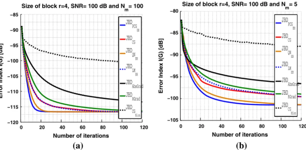
We considerM = N = 8 (Ais square) andr =4 (withr =4 for all j =1, . . . ,4). The setMofNmsquare matricesMi,i=1, . . . ,Nmconsists ofNm=100 (resp.Nm=5)

M×Mmatrices. All algorithms are initialized using the same initialization provided by the generalized eigenvalue decomposition (GEVD) as suggested inNion 2011. Notice that the maximal number of iterations allowed is set atNmax=120 iterations.

The evolution of the error index versus the number of iterations is illustrated emphasizing the influence of i) the numberNmof matrices to be block diagonalized, ii) andSNR. In fact,

two cases are considered: i) on the leftNm=100 ii) and on the rightNm=5 for the considered

matrices set. In addition, we illustrate in the Fig.1(resp. the Fig.2) the evolution of the error index versus the number of iterations in the noiseless case (SNR=100 dB) (resp. the noisy case (SNR=30 dB)).

From these curves, several observations can be drawn. First we observe that the conver-genceofalgorithmsbasedonanexactpreconditioningnamelyJBDPCGEH,JBDLMEH and

JBDQNEHare the fastest algorithms. Moreover, comparing the convergence of different

gra-dient approaches namely JBDCGNIONand JBDRGrad, we check the interest of our proposed

preconditioner based on the exact Hessian matrices. Furthermore, we deduce that the conver-gence speed of the algorithm JBD_CG is higher than JBDRGrad, JBDAbsGrad and especially

the algorithm JBDCGNIONwhich follows the same adaptation rule but operates on a different

costfunction.However,thebestperformancesaregenerallyachievedusingtheJBDPCGEH

algorithm in difficult contexts: with noise and a set containing a small number of matrices to be joint block diagonalized. In addition, we note that JBDPCGEHand JBDQNEHconverge

0 20 40 60 80 100 120 −120 −115 −110 −105 −100 −95 −90 −85

Number of iterations Number of iterations

Size of block r=4, SNR= 100 dB and N m= 100 JBD PCG EH JBD CG JBD QN EH JBD LM EH JBD AbsGrad JBD RGrad JBD CG Nion (a) 0 20 40 60 80 100 120 −105 −100 −95 −90 −85 −80

Error Index I(G) [dB]

Error Index I(G) [dB]

Size of block r=4, SNR= 100 dB and N m= 5 JBD PCG EH JBD CG JBD QN EH JBD LM EH JBD AbsGrad JBD RGrad JBD CG Nion (b)

Fig. 1 Comparison of the different algorithms: evolution of the error indexI(G)versus the number of iterations in the noiseless case (SNR=100 dB) for different sizes of the matrix sets.aNm=100,bNm=5

0 20 40 60 80 100 120 −50 −45 −40 −35 −30 −25 −20 −15

Size of block r=4, SNR= 30 dB and N m= 100

Number of iterations

Error Index I(G) [dB]

JBD PCG EH JBD CG JBD QN EH JBD LM EH JBD AbsGrad JBD RGrad JBD CG Nion (a) 0 20 40 60 80 100 120 −35 −30 −25 −20 −15 −10

Size of block r=4, SNR= 30 dB and N m= 5 Number of iterations JBD PCG EH JBD CG JBD QN EH JBD LM EH JBD AbsGrad JBD RGrad JBD CG Nion (b)

Error Index I(G) [dB]

Fig. 2 Comparison of the different algorithms: evolution of the error indexI(G)versus the number of iterations in the noisy case (SNR=30 dB) for different sizes of the matrix sets.aNm=100,bNm=5

to the same solution approximately. However, the others require more iterations to reach the same performances.

We observe also that the more matrices to be joint block-diagonalized we have, the best the obtained results are. In addition, whatever the considered algorithm, they all reach the same level of performance (which not too surprising either), yet, theJBDCGNION,JBDRGradand

JBDAbsGradalgorithms need more iterations. Even though when smaller subsets of matrices

and theSNRvalue are considered, the results remain relatively good. Not too surprisingly, the noise affects the performances.

6 Application to blind source separation

In this section, we show how to use the proposedJBDalgorithms for solving the FIR con-volution of non-stationary sources. We recall that the principle of theBSSproblem is to

restore multiple sources mixed through an unknown mixing system that we must estimate from the system outputs only called “the observations”‘. To do this, we are basically inter-ested in methods based on spatial time-frequency distributions or spectra. It is well known that this kind ofBSSmethods generally need four main steps to guarantee successful signal separation.

6.1 The matrix model of the source separation problem

Consideringm(m ∈N∗) observation signalsxi(t), i =1, . . . ,m, t ∈Z, andn(n∈N∗)

sourcessj(t), for allj=1, . . . ,nwhich are mixed through a linearFIRmultichannel system

and represented byH(t)=(Hi j(t)). The convolutive model can be simply described by the

following expression : xi(t)= n j=1 L =0 Hi j( )sj(t− )+nj(t), (32)

whereHi j(t)is the impulse response function between thei-th sensor andj-th source with an

overall extent ofL+1 taps andni(t), for alli =1, . . . ,mare noises. Hence, the convolutive

system can be written as an instantaneous model of source separation problem:

X(t)=AS(t)+N(t), (33) where:

– The(M×N)mixing matrixAis a block-matrix given byA=Ai j

for alli=1, . . . ,m

and j=1, . . . ,nwhose blocksAi jare(L×Q)Toeplitz matrices:

Ai j= ⎛ ⎜ ⎜ ⎜ ⎜ ⎝ Hi j(0) . . . Hi j(L) 0 . . . 0 0 ... ... ... ... ... ... ... ... ... ... 0 0 . . . 0 Hi j(0) . . . Hi j(L) ⎞ ⎟ ⎟ ⎟ ⎟ ⎠. (34)

– The(N ×1)vectorS(t)= [s1(t)T,s2(t)T, . . . ,sn(t)T]T containing sources where the

(Q×1) vectorssi(t)(for alli=1, . . . ,n) stands forsi(t)= [si(t),si(t−1), . . . ,si(t−

Q+1)]T,

– The (M ×1) vectorX(t) = [x1(t)T,x2(t)T, . . . ,xm(t)T]T (resp.N(t) = [n1(t)T, n2(t)T, . . . ,nm(t)T]T) containing the observed signals (resp. the noise signals) where the

(L×1) vectorsxi(t)(resp.ni(t)) stands forxi(t)= [xi(t),xi(t−1), . . . ,xi(t−L+1)]T

(resp.ni(t)= [ni(t),ni(t−1), . . . ,ni(t−L+1)]T),

– M =m L,N =n(L+L) =n Q(withQ = L+LandL ∈N∗) and Lis chosen such thatM≥N to maintain an over-determined model.

We assume that the noises are stationary, white, centered random signals, mutually uncor-relatedandindependentfromthesourcesignals.

6.2Constructionofthet-f matricessettobejointblock-diagonalized

The Spatial Quadratic Time-Frequency Spectrum (SQTFS) of the observations across the array at a given t-f point is a (M×M)matrix, admits the following decomposition:

DX(t, ν)=ADS(t, ν)AH+DN(t, ν)+ADSN(t, ν)+DNS(t, ν)AH

=ADS(t, ν)AH+DN(t, ν), (35)

where,

– DS(t, ν)(resp.DN(t, ν)) is the (N × N)source SQTFS (resp. the(M× M) noise SQTFS).

– DSN(t, ν)andDNS(t, ν)are the Spatial Bilinear Time-Frequency Spectrum (SBTFS) between the sources and the noises. TheseSBTFSare null since the noises are indepen-dent from the source signals.

We have to recall a very important property, as expressed inGhennioui et al. 2010, which allows to solve theBSS problem such that the matrixDS(t, ν)takes a specific algebraic structure. In fact, it is block-diagonal with one single non null(Q×Q) block on the block-diagonal. Moreover, the block-diagonal matrix with one single non null block is the only possibility of block-diagonal matrix when these matrices outcome of spatial time-frequency distributions or spectrum (SQTFD(orS)).

In order to build the set of matrices denotedMJBDfor joint block-diagonalization. We

fol-low the same procedures for the detector proposed inGhennioui et al. 2010denotedCConvGH.

All the matrices from the setMJBDadmit the decomposition given by equation (35) or (1)

(after the noise reducing processGhennioui et al. 2010), where the sourceSQTFD(orS) matricesDS(t, ν)assume a very specific algebraic structure (block diagonal matrices). As a result, to tackle theBSSproblem, we use our proposedJBDalgorithms.

6.3 Estimation of the separation matrix

The matrices belonging to the setMJBD of sizeNm (Nm ∈ N∗) can be decomposed into

ADS(t, ν)AH withDS(t, ν)a block-diagonal matrix with only one non null (Q×Q) block on its block-diagonal. One possible way to be able to recover the mixing matrixA(or its pseudo-inverse: the separation matrixB) is to directly joint block diagonalize the matrices setMJBD. As known, the sources recovered are obtained up to a permutation and up to a

filter which are the classical indeterminations of theBSSin the convolutive context. FourBSSmethods can be then derived: the first one is denotedJBDPCGEH−TFsince it

com-bines theJBDalgorithm based on a preconditioned conjugate gradient approachJBDPCGEH

together with the automatic time-frequency points detectorCConvGH. The three other

meth-ods denoted respectivelyJBDQNEH−TF,JBDLMEH−TF andJBDCGTF consist of replacing the

preconditioned conjugate gradient-basedJBDalgorithm by respectively the Quasi-Newton algorithmJBDQNEH, the Levenberg–Marquardt algorithmJBDLMEHand the conjugate

gra-dient algorithmJBDCG. 6.4 Computer simulations

In this section, computer simulations are performed in order to illustrate the good perfor-mance of the four suggested methods and to compare them again with the same kind of existing approaches: the first one is denoted byJBDCGNION−TFand combines the non-unitary

JBDalgorithm proposed inNion 2011with thet-f point detectorCConvGH. The other

algo-rithms denotedJBDRGrad−TF andJBDAbsGrad−TF combine respectively the non-unitary

JBDalgorithm proposed inGhennioui et al. 2010and the non-unitaryJBDalgorithm pro-posed inGhennioui et al. 2008awith the same detector.

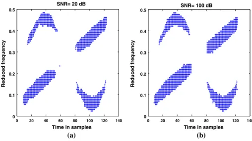
We considerm = 4 mixtures ofn = 2 sources of 128 time samples. The first source (resp. the second source) is a sinusoidal frequency modulation (resp. a linear frequency

0 20 40 60 80 100 120 140 0 0.1 0.2 0.3 0.4 0.5 Time in samples Reduced frequency SNR= 20 dB (a) 0 20 40 60 80 100 120 140 0 0.1 0.2 0.3 0.4 0.5 Time in samples Reduced frequency SNR= 100 dB (b) Fig. 3 The selectedt-fpoints with automatic points detectorC_Conv

GH

modulation),L=3 andL=2. These sources are mixed according to a mixture matrixA(t)

whose components were randomly generated and whose z-transformA[z]is given by:

⎛ ⎜ ⎜ ⎝ −0.0134+0.2221z−1+0.9749z−2 −0.6579+0.7521z−1−0.0382z−2 −0.7425−0.6639z−1_−0.0891z−2 _{0.7287+0.6049z}−1_−0.3210z−2 0.6173+0.3921z−1−0.6820z−2 0.9477−0.2211z−1−0.2301z−2 0.7119−0.6532z−1_−0.2578z−2 _{0.2533−0.7511z}−1_−0.6096z−2 ⎞ ⎟ ⎟ ⎠,

We use the Spatial Pseudo Wigner-Ville Spectra (SPWVS) with a Hamming smoothing window of size 128 and 64 frequency bins. In this example, 30 realizations of signals are computed. Then, theSPWVSof each realization is calculated. For the noises, we use random entries chosen from a Gaussian distribution with zero mean and varianceσ2

N.

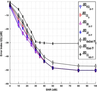
In the Fig.4, we have plotted the error indexI(G)versus theSNR(≈1410 time-frequency matrices were selected whenSNR≥20 dB (see the Fig.3for the selectedt-fpoints). In fact, the more theSNRdecreases (forSNR≤20 dB), the more the performance decreases too. The resulting error index shows that the four proposed methods show the best performances. We observe again that the performances of proposed algorithms based on an exact precon-ditioning namelyJBDPCGEH−TF,JBDQNEH−TF andJBDLMEH−TF are the fastest algorithms.

TheJBDCGTF method still performs better thanJBDCGNION−TF based on conjugate

gradi-ent and which exhibits, in this simulation, the worst performances especially in the noisy context. However, theJBDPCGEH−TF andJBDQNEH−TFmethods that provide the best results

in the same context. Finally, allt-f methods reach the same performances especially when SNR≥40 dB except, logically,JBDCGNION−TF which operates on a different cost function

Nion 2011.

7 Discussion and conclusion

In this article, we are interested in non unitary joint block diagonalization problem which is of great interest in different fields of application such that array processing for wide-band signals and blind sources separation when convolutive mixtures are considered. Our

0 10 20 30 40 50 60 70 80 90 100 −60 −50 −40 −30 −20 −10 0 SNR [dB]

Error Index I(G) [dB]

JBD

JBD

JBD

JBD

JBD

JBD

JBD

Fig. 4 Comparison of the different algorithms in the BSS context: evolution of the error indexI(G)versus the SNR

aim, here, was to investigate the relevance/interest of a preconditioning for those algorithms. Such a procedure usually requires either the calculation of the exact complex Hessian matrix at each iteration. In this article, the exact calculation has been performed. Then, different iterative preconditioned joint block diagonalization algorithms have been derived and com-pared. We have focused our attention on Quasi-Newton, Preconditioned Conjugate Gradient and Levenberg–Marquardt algorithms. Computer simulations presented in difficult contexts (noise and/or very few matrices to be joint block diagonalized) have emphasized the good behavior of the preconditioned conjugate gradient algorithm. This algorithm offers the best compromise between good performance and fast convergence speed even in complicated scenarios. The main advantage of the approach suggested here remains its really general aspect. In fact, it does not rely on restrictive assumptions neither about the considered matrix set (they only have to be complex but not necessarily hermitian matrices) nor about the joint block-diagonalizer (it is not necessarily an unitary matrix). Finally, we have used the proposed algorithms to show their usefulness in theBSScontext. All these algorithms have brought four time-frequency basedBSSmethods combined with at-fpoints detectorCConvGH.

Appendix A: Calculation of the complex Hessian matrices

We consider three square matrices,D1,D2andD3inCM×M and five rectangular matrices

D4,D5,D6inCN×M,D7inCM×NandD8inCF×G. Lettr{·},d(·)(or sometimes simplyd), vec(·),OffBdiag_(n){·}andTBoffrespectively denote the trace operator of a square matrix, the differential operator, the vectorization operator that stacks the columns of a matrix in a

long column vector, the zero-block-diagonal operator defined inGhennioui et al. 2010and the N2_×N2_{“transformation” matrix defined before. Our developments are based on the}

following properties (they can be found in (Ghennioui et al. 2010;Hjorungnes, A. 2011; Brewer 1978) orMagnus and Neudecker 1999b):

P0. OffBdiag₍n){D1}2F=tr DH 1OffBdiag(n){D1} . P1. (D4+D5)T =DT₄ +DT₅. P2. (D4D7)T =D7TD4T. P3. (D4D7)∗=D∗₄D∗₇. P4. tr{D1+D2} =tr{D1} +tr{D2}. P5. tr DH₄D5 =(vec(D4))Hvec(D5). P6. d(tr{D1})=tr{d(D1)}.

P7. vec(D1D2D3) = (DT3 ⊗ D1)vec(D2) ⇒ vec(D1D2) = (IN ⊗ D1)vec(D2)

=(DT₂ ⊗IN)vec{D1}

P7b. vec(D4D1D7) = (DT₇ ⊗ D4)vec(D1) ⇒ vec(D4D1) = (IM ⊗ D4)vec(D1)

=(DT₁ ⊗IN)vec{D4}

P8. vec

D₄T=KN,Mvec(D4)withKN,Mthe unique squareN M×N Mcommutation

matrix defined as:KN,M= N

n M

m Enm⊗ETnmwhereEnmareN×Mmatrices with

a 1 in the(n,m)position and zeros elsewhere:(Enm)=(δnm)(δnmstanding for the

Kronecker Delta). As a consequence, the permutation matrixKN,Mhas one single “1”

in each row and in each column.

P8b. KN,MKM,N =IM N andKN,M =K−M1,N =KTM,N.

P9. vec(OffBdiag{D1})=TBoffvec(D1). P10. d(vec(D4})=vec(d(D4)). P11. d(D4+D5)=d(D4)+d(D5). P12. d(D4D7)=d(D4)D7+D4d(D7). P13. dD∗₄=d(D4)∗. P14. tr{D1)=trDT₁. P15. (D4⊗D8)T =DT4 ⊗DT8. P16. (D4⊗D8)H =D₄H⊗D₈H.

P17. vec(D4+D5)=vec(D4)+vec(D5). P18. D4H = D∗₄T. P19. (D4D7)H =D7HD4H. P20. (D1⊗D2) (D3⊗D7)=(D1D3⊗D2D7). P21. (D4+D5)H=D₄H+DH₅.

P22. OffBdiag_(n){D1+D2} =OffBdiag_(n){D1} +OffBdiag_(n){D2}.

P23. dD∗4=(dD4)∗.

According to Hjorungnes, A. 2011, the first-order differential of the cost function CJBD(B,B∗)defined in (3) is given by:

dCJBD(B,B∗)=DB CJBD(B,B∗) dvec(B)+DB∗ CJBD(B,B∗) dvec(B∗), (36) if the 1×N Mcomplex vectorsDB(CJBD(B,B∗))andDB∗(CJBD(B,B∗))are defined as:

DB CJBD(B,B∗) =vecT ∂CJBD(B,B∗) ∂B , DB∗ CJBD(B,B∗) =vecT ∂CJBD(B,B∗) ∂B∗ . (37)

We also recall that the two partial derivatives that are involved i.e. ∂CJBD_∂B(B,B∗) and ∂CJBD(B,B∗₎

∂B∗ were calculated inGhennioui et al. 2010using some of the previous

proper-tiesP0-P20. They were found to be equal to:

∂CJBD(B,B∗) ∂B = Nm i=1 OffBdiag₍n){BMiBH} T B∗M∗_i +OffBdiag₍n){BMiBH} ∗ B∗M_iT , (38) ∂CJBD(B,B∗) ∂B∗ = Nm i=1 OffBdiag_(n){BMiBH}BMiH+ OffBdiag_(n){BMiBH} H BMi = ∂CJBD(B,B∗) ∂B ∗ . (39) DB∗ CJBD(B,B∗) =(DB(CJBD(B,B∗)))∗. (40)

As shown inHjorungnes, A. 2011, the second order differential is then given by:

d2CJBD(B,B∗)=dDB CJBD(B,B∗) dvec(B)+dDB∗ CJBD(B,B∗) dvec(B∗). (41) Thus, we have to evaluate the differential of the two derivativesDBandDB∗,i.e. dDBand

dDB∗. We start withdDB. Using the propertiesP2,P3,P10-P14,P17-P19in (38), we have: dDB CJBD(B,B∗) = Nm i=1 vecT OffBdiag_(n){dB∗M_iTBT} B∗M∗_i +OffBdiag_(n){B∗MT_i dBT} B∗M_i∗ +vecT OffBdiag_(n){dB∗M∗_iBT} B∗MT_i +OffBdiag_(n){B∗M∗_idBT} B∗MT_i +vecTOffBdiag_(n){BMiBH} T dB∗M∗_i + OffBdiag_(n){BM_iHBH} T dB∗M_iT . (42)

Then, using the propertiesP1,P7, andP17we obtain:

dDB CJBD(B,B∗) = Nm i=1 B∗M∗_iT ⊗IN vec OffBdiag_(n){dB∗M_iTBT} +B∗M∗_iT⊗IN vec OffBdiag_(n){B∗MT_i dBT} +B∗M_iT T ⊗IN vec OffBdiag_(n){dB∗M∗_iBT} +B∗M_iT T ⊗IN vec OffBdiag_(n){B∗M∗_idBT} + IN ⊗ OffBdiag_(n){BMiBH} T M_iH⊗IN vecdB∗

+ IN ⊗ OffBdiag_(n){BM_iHBH} T (Mi⊗IN)vec dB∗ T . (43) While propertiesP2,P3,P7,P8,P9, andP18involve:

dDB CJBD(B,B∗) = Nm i=1 M_iHBH⊗IN TBoff(BMi⊗IN)vec(dB∗) +M_iHBH⊗IN TBoff IN ⊗B∗MiT KN,Mvec(dB) +MiBH⊗IN TBoff BM_iH⊗IN vec(dB∗) +MiBH⊗IN TBoff IN ⊗B∗Mi∗ KN,Mvec(dB) + IN⊗ OffBdiag_(n){BMiBH} T M_iH⊗IN vec(dB∗) + IN⊗ OffBdiag_(n){BM_iHBH} T (Mi⊗IN)vec(dB∗) T . (44) The propertiesP1,P2,P3,P15,P16,P17,P18,P19, andP20imply the following result:

dDB CJBD(B,B∗) = Nm i=1 vecT(dB) KN,M T IN⊗MiBH TT_BoffB∗M∗_i ⊗IN +KN,M T IN⊗MiHBH TT_Boff B∗MT_i ⊗IN ! +vecTdB∗ MT_i BT ⊗IN T_BoffT B∗M∗_i ⊗IN +M_i∗BT⊗IN TT_Boff B∗M_iT⊗IN +M_i∗⊗ OffBdiag_(n){BMiBH} +M_iT⊗ OffBdiag_(n){BM_iHBH} ! . (45)

Finally this 1×N Mvector can be rewritten as follows:

dDB

CJBD(B,B∗)

=dvecT_(B∗_)dvecT_(B) A00

A10

, (46)

which leads to the expressions ofA00andA10given in (12)-(13).

Concerning the second differentialdDB∗, we are taking advantage of (40). Using property

P23, we finally havedDB∗ =(dDB(CJBD(B,B∗)))∗, which leads to: dDB∗ CJBD(B,B∗) =dvecT(B)dvecT(B∗) A∗00 A∗₁₀ . (47)

But this 1×N Mvector was supposed to be written as:

dDB∗

CJBD(B,B∗)

=dvecT_(B∗_)dvecT_(B) A01

A11

, (48)