MPRA
Munich Personal RePEc Archive
Introducing the Net Present Value
Profile
Peter Bell
17 June 2017
Online at
https://mpra.ub.uni-muenchen.de/79764/
Abstract
The Net Present Value is an important statistic in the evaluation of investment opportunities. Analysts often consider the sensitivity of NPV to different parameters in an economic model, but always seem to consider the NPV of a project at the single instant before the project is launched. This short note introduces the idea of a NPV Profile, which shows how the NPV of a project changes over the life of that project. The note calculates the NPV Profile for a simplified cash flow model and briefly discusses how this statistic can be used to consider returns in possible takeover scenarios.
Keywords: Net Present Value, Project Valuation, Takeovers
The Net Present Value (NPV) is a basic building block in mathematical economics. It is used in the investment industry for the valuation of projects, such as the development of a mine. Analysts generally focus on NPV at initial period before the project has been launched and, in doing so, overlook how the NPV of the project may change over time. This paper considers how the NPV may change over the life of project in a simplified setting.
To begin, I present the Cash Flow Profile for a hypothetical project. Figure 1 shows the net cash flow on an annual basis. Note that the project begins with negative cash flow in Year 1 and then then provides positive cash flow over an extended period. The project ends with zero cash flow for simplicity. This stylized Cash Flow Profile is meant to represent a “good” mine project with long mine life.
I created this Cash Flow Profile to have certain stylized features. One such feature is that the initial NPV is slightly greater than the initial capital expenditure. To achieve that, I set the initial expenditure equal to $100 and annual cash flow $30. Another such feature is that the project has a sufficiently long life that the terminal period contributes a small amount to initial the NPV. To achieve that, I set the terminal period as Year 30. This Cash Flow Profile is meant to be a generous but not unrealistic description of a good mining project.
The following table contains some summary information regarding this project. As shown in this table, the initial expenditure of $100, initial NPV of $140, Internal Rate of Return (IRR) is 24%, and payback period is 3.33 Years. Again, these conventional statistics provide further evidence that the project has strong economics.
Initial Capital Expenditure
($) Annual Cash Flow ($) Initial NPV ($) IRR (%) Payback period (Years)
100 30 140 24% 3.33
The NPV Profile is calculated as the NPV from a particular base year through to the end of the project’s life across a series of base years. I denote the NPV at time t as NPV(t) and calculate the NPV Profile as follows:
𝑁𝑃𝑉(𝑡) = ∑ 𝐶𝐹(𝑖) (1 + 𝑟)𝑖 𝑇
𝑖=𝑡
Where CF(i) denotes cash flow at time i, and r is the discount rate. I assume the discount rate r=10% for simplicity.
Figure 2 shows the NPV Profile for the Cash Flow Profile above. As in the table above, the initial NPV is $140. However, things get a bit more interesting after that.
begins. The NPV peaks at $280 in year 3, which is the same time that cash flow begins. At its peak, the NPV is twice as large as the initial NPV. The NPV increases in this way because the initial expenditures have already been incurred and the valuation is based solely on the positive cash flow. However, the NPV decreases after that time as the end of the project becomes more near.
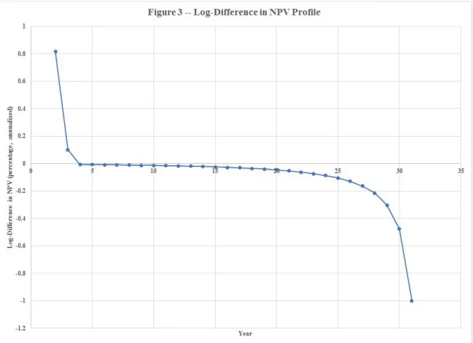
Figure 3 shows the rate of change of NPV Profile. I refer to it as the “log-difference in NPV profile” because it shows the percentage change in NPV profile each year.
As noted above, the NPV increases very quickly at the start of the project: the NPV actually increases by over 80% after the expenses are made in the first year. However, the NPV starts to decrease after that as the end of the project approaches and ultimately decreases by -100% in the final year.
Figure 4 shows the second derivative of the NPV Profile, which is calculated as a percentage change. This figure shows that the initial increase in the NPV Profile is deaccelerating and but the subsequent decrease in NPV is accelerating.
In conclusion, I believe that the NPV Profile can be used in several ways. For one, it can be used to explore the potential valuation of the project in a simplified takeover scenario. This discussion can get a little complicated based on the assumptions that go along with it, but I believe the NPV Profile can be helpful for providing an additional dimension to the modelling of the financial returns associated with the project.
If you owned the project and only had to incur the initial expenditures of $100, then you could earn a greater return by selling it in Year 3 than holding it to termination. Specifically, you would have paid $100 in Year 1, received $0 in Year 2, and sold the project for $280 in Year 3, which provides an IRR of 67%. However, if you also had to buy the project for the initial NPV of $140 in Year 1, then things look a bit different. You would have paid $240 in Year 1 and your IRR would be 8%, which is lower than the 24% IRR associated with holding the project to termination.
I suspect that the NPV Profile can be used in other ways, such as comparing different projects with the same initial NPV. I would encourage researchers to explore this line of thinking and to develop the connection between the NPV Profile and the valuation of projects based on multiples of cash flow, which is an important method that is mathematically related to the NPV formula.
Time Cash Flow NPV D-NPV D2-NPV 1 -100 $139.83 2 0 $253.82 0.82 3 30 $279.20 0.10 -0.88 4 30 $277.12 -0.01 -1.07 5 30 $274.83 -0.01 0.11 6 30 $272.31 -0.01 0.11 7 30 $269.54 -0.01 0.11 8 30 $266.50 -0.01 0.11 9 30 $263.15 -0.01 0.11 10 30 $259.46 -0.01 0.11 11 30 $255.41 -0.02 0.12 12 30 $250.95 -0.02 0.12 13 30 $246.04 -0.02 0.12 14 30 $240.65 -0.02 0.12 15 30 $234.71 -0.02 0.12 16 30 $228.18 -0.03 0.13 17 30 $221.00 -0.03 0.13 18 30 $213.10 -0.04 0.14 19 30 $204.41 -0.04 0.14 20 30 $194.85 -0.05 0.15 21 30 $184.34 -0.05 0.15 22 30 $172.77 -0.06 0.16 23 30 $160.05 -0.07 0.17 24 30 $146.05 -0.09 0.19 25 30 $130.66 -0.11 0.21 26 30 $113.72 -0.13 0.23 27 30 $95.10 -0.16 0.26 28 30 $74.61 -0.22 0.32 29 30 $52.07 -0.30 0.40 30 30 $27.27 -0.48 0.58 31 0 $0.00 -1.00 1.10