CEP Discussion Paper No 748
August 2006
Assessing the Effects of Local Taxation
Using Microgeographic Data
Gilles Duranton, Laurent Gobillon
and Henry G. Overman
Abstract
We study the impact of local taxation on the location and growth of firms. Our empirical methodology pairs establishments across jurisdictional boundaries to estimate the impact of taxation. Our approach improves on existing work as it corrects for unobserved establishment heterogeneity, for unobserved time-varying site specific effects, and for the endogeneity of local taxation. Applied to data for English manufacturing establishments we find that local taxation has a negative impact on employment growth, but no effect on entry.
Keywords: Local taxation, spatial differencing, borders JEL Classifications: H22, H71, R38
Data: ARD, British Local Election Database
This paper was produced as part of the Centre’s Globalisation Programme. The Centre for Economic Performance is financed by the Economic and Social Research Council.
Acknowledgements
Thanks to Tom Davidoff, Tom Holmes, Thomas Klier, Thierry Mayer, John Quigley, Helen Simpson and to seminar and conferences participants in Berkeley, Boston, Ghent, Glasgow, Hamburg, Kansas City, Kiel, Kyoto, London, Paris, Seattle, Vancouver, and Venice. We also owe special gratitude to Tim Besley. Financial support from the Economic and Social Research Council (Grant R000239878) and the Leverhulme Trust is gratefully acknowledged. This paper uses data that are Crown Copyright and reproduced with the permission of the HMSO Controller and the Queen's Printer for Scotland. However, the use of these data does not imply ONS endorsement of either the interpretation or the analysis in this paper.
Gilles Duranton is an Associate member of the Centre for Economic Performance, London School of Economics; Associate Professor of Economics and Noranda Chair in International Trade and Development at the University of Toronto, Canada and a CEPR Research Affiliate. Email: [email protected]. Laurent Gobillon is a Researcher at the French Institute of Demographics (Institut National d’Etudes Démographiques, INED). He is also an Associate Researcher at the London School of Economics. Email: [email protected]. Henry G. Overman is an Associate member of the Centre for Economic Performance, London School of Economics; Lecturer in the Department of Geography and Environment, LSE and a CEPR Affiliate. Email: [email protected]
Published by
Centre for Economic Performance
London School of Economics and Political Science Houghton Street
London WC2A 2AE
All rights reserved. No part of this publication may be reproduced, stored in a retrieval system or transmitted in any form or by any means without the prior permission in writing of the publisher nor be issued to the public or circulated in any form other than that in which it is published.
Requests for permission to reproduce any article or part of the Working Paper should be sent to the editor at the above address.
© G. Duranton, L. Gobillon and H. G. Overman, submitted 2006 ISBN 0 7530 2054 8
1. Introduction
This paper develops new empirical methodologies to provide evidence on the effects of local taxation on the location and growth of firms. This issue has been the focus of an extensive theoretical literature and our paper is clearly not the first paper to consider these issues empirically.1 Bartik (1991) summarises results from the earlier literature. Evidence from the 1960s and 1970s suggested there was no effect of taxes on firm location decisions. Bartik’s own work focusing on the 1980s suggested that there was a negative relationship and a number of subsequent papers have confirmed that general finding. Much of this work used fairly large spatial units (mostlyUSstates). More recent work (e.g., Guimaraes, Figueiredo, and Woodward, 2004) has started to move towards smaller spatial units such asUScounties with similar results.
The existing literature, however, has failed to satisfactorily resolve three main problems when attempting to assess this impact. First, firms are faced with a choice of a large number of heterogenous locations when deciding where and how to produce. Many of these site characteristics are unobserved and are likely to be correlated with other explanatory variables such as plant characteristics and local taxation, thus biasing the results. Second, firms themselves are also heterogenous. Again much of this heterogeneity is unobservable so that the sorting of firms according to these characteristics provides another possible source of bias. Third, some aspects of the tax system may be endogenous to firm production and location decisions, which may lead to a reverse causality bias.
This paper attempts to deal with all three of these problems. The crux of our approach is to use spatial differencing between neighbouring firms across borders to control for the first source of bias. Incorporating standard panel and instrumental variable techniques
1One can identify at least three strands of theoretical literature. The issue of tax competition has received
considerable attention with the race to the bottom argument prominent in many discussions. See Wilson (1999) for a review. A similarly lengthy debate has centred around the issue of local public good provision and the Tiebout (1956) hypothesis that inter-jurisdictional competition helps achieve the efficient provision of local public goods. See Epple and Nechyba (2004) for a recent review. Finally, capitalisation of local taxes and the possibility of the efficient taxation of land are key concerns for urban economists. This has been a subject of discussion since George (1884). See Fujita (1989) for a thorough presentation of the arguments and Arnott (2004) for a recent discussion of its applicability.
then allows us to deal with the other two possible biases. When applying the resulting methodology to data for English manufacturing establishments we find that local taxation has a negative impact on employment growth, but no effect on entry. We also show that standard methodologies that do not address these three key problems give substantively different results.
The rest of the paper is structured as follows. In section 2 we outline our methodology and relate it to the existing literature. Section 3 outlines our data. Section 4 presents our findings on the impact of local taxation on employment while section 5 presents results on entries. Section 6 concludes.
2. Methodology
A. Heterogenous locations
When locating, establishments are faced with a large number of heterogenous sites.2 These sites come at very different rental prices. For instance, Thompson and Tsolacos (2001) document a sixfold difference in the rental price per square metre between indus-trial sites close to Heathrow airport and those in the suburbs of Leeds. Once located, many variables may then impact on production decisions. Traditional empirical approaches have worried about the fact that the costs of labour and other factors of production differ across geographical regions. We will address this issue, but are also concerned with heterogeneity at a much finer geographical scale. A wide variety of factors will affect both the attractiveness of particular sites and the success of establishments once they have chosen their site. For example, the attractiveness of a site may depend on access to the road network while changes to that network may affect the performance of establishments at that site. Hence, we expect considerable site heterogeneity, possibly at a very fine spatial scale, and this heterogeneity may well vary over time.
2We use the term establishments to refer to our basic units of observation. In the data that we use, these
If this is the case, assessing the impact of local taxation will require us to control for both fixed and time-varying site characteristics since they are likely to be correlated with local taxes or other establishment characteristics. Some of these site characteristics may be observable and thus can be controlled for directly. However many are likely to be unobservable. Because we expect unobserved site characteristics to vary smoothly across space, neighbouring sites are likely to have similar values of these unobserved characteristics. Within jurisdictions, neighbouring sites also have similar tax rates. This raises the possibility that unobserved site characteristics may be correlated with the very variable in which we are interested. Unobserved site characteristics are also potentially correlated with establishment characteristics if, for instance, better establishments tend to locate on better sites. Thus, for example, if more productive owners help to ensure establishment survival and also choose better sites then age may be correlated with unob-served site characteristics. More complex interactions are also possible if establishments sort according to both site characteristics and taxation. For these reasons, dealing with these unobservable site characteristics is the first key step in developing a methodology to assess the impact of local taxation.
A typical solution to this problem would be to assume that the unobservable effects are common across siteswithinjurisdictions and to include dummy variables to condition out these effects. Using longitudinal data, these jurisdictional dummies should pick up any unobserved, time-invariant fixed effects common to all establishments in the jurisdiction.3 For unobserved site characteristics that vary strongly across jurisdictions (as a result, for instance, of very different institutional contexts), the assumption that unobserved effects are constant within jurisdictions may be a natural one. Our approach will control for such differences. However, to assess the impact of local taxation within a given institutional context, this is unlikely to be sufficient since many, if not most, unobserved site character-istics are likely to vary within juridictions and across time.
3In the location literature this approach has proved difficult to implement in situations with a large
number of jurisdictions, because non-linear models (e.g., conditional logit) do not allow one to difference out the large number of dummy variables before estimation. See section 5 for further discussion.
The novelty in our approach is to exploit the fact that, although unobserved site characteristics vary across space, they are likely to be highly spatially correlated. Using ideas from Holmes (1998) we identify establishments that are close to one another, but on different sides of jurisdictional boundaries.4 Because of the spatial correlation in site characteristics, these establishments will have very similar unobserved site characteristics, but will face different tax rates. We look at the extent to which differences in employment between these pairs of establishments can be explained by different local tax rates. This spatial differencing allows us to control for unobserved site characteristics, be they fixed or time-varying. Hence, compared to standard approaches, ours has the added advantage that it can control for variations in site characteristics that occur within jurisdictions as well as the fact that these unobserved effects may vary over time.
B. Heterogenous establishments
We also expect production establishments to be very heterogenous and much of this heterogeneity to be unobservable. This is a second likely source of bias if establishments with different unobserved characteristics sort across jurisdictions with different tax rates.
Our approach to dealing with the existence of heterogenous establishments is more standard. Because we have a panel of establishment level data, we are able to control for observed time-varying characteristics of establishments, as well as condition out unobserved time-invariant characteristics through the inclusion of establishment fixed effects. Note that the inclusion of establishment fixed effects should also control for unobserved time-invariant site-specific effects (if establishments do not move) leaving our spatial differencing to control for unobserved time-varyingsite-specific effects. Although there is nothing particularly innovative in the method we use to deal with establishment
4See also Black (1999). The methodology proposed by Holmes (1998) and Black (1999) has been repeated
elsewhere, but most applications only use cross-sectional data and do not address endogeneity issues. The two exceptions are Gibbons and Machin (2003) who consider endogeneity and Kahn (2004) who uses some longitudinal information. As will become clear below, our analysis improves on these existing methodolo-gies by incorporating instrumented panel data techniques into the spatial discontinuity approach.
heterogeneity, as far as we are aware panel data techniques have not been used in the existing literature on the impact of local taxation.5
C. The endogeneity of taxation
Another issue that we need to confront is the endogeneity of tax rates to employment and location decisions. To do this, we will argue that the nature of the UK business rates system (the local tax that we consider in this paper) allows us to instrument the levels of local taxation by local political variables. We provide further details below.
D. A model of the employment impact of local taxation
To make this discussion concrete, we consider the impact of local taxation on establish-ment employestablish-ment decisions (the main focus of this paper). Because the specific tax that we look at in this paper, the UKbusiness rates, is essentially a property tax that applies to all commercial properties, we model it as changing the rental cost of buildings.
Take location as given.6 The establishment occupies one of many sites indexed by z. The jurisdiction that sets the tax for this establishment depends on the site occupied. Jurisdictions are indexed bya.
Establishments use buildings, K, and labour, L, to produce a final good. We take the final good as numeraire and assume that the price is common across all jurisdictions. The wage rate, wz, is site-specific. The rental cost of building comprises two elements: the
rent, τz, which is site-specific, and the tax, ra, which may vary across jurisdictions. This
specification mirrors the working of theUKrates system as described below. Note that this specification is very flexible and allows for establishments to face site-specific factor costs. Ignoring time subscripts for simplicity, the establishment’s profit maximisation problem
5Berman and Bui (2001) use panel data methods to estimate the effects of local environmental regulations
(but not taxes) on the labour demand ofUSoil refineries.
6Allowing establishments to chose location involves a simple extension. The problem can be solved
backward through a two-stage maximisation. First, calculate maximum profits at each location. Second, maximise with respect to location. See section 5 for further details.
can be written as:
MaxLi,KiΠi = AiBaF(Li,Ki)−wzLi−(1+ra)τzKi (1)
whereFis the production function,Aiis an establishment-specific productivity effect, and
Ba is a jurisdiction productivity effect. Under standard regularity conditions, a sufficient
condition for profit maximisation is that the following first-order conditions hold: ∂Πi ∂Li = AiBa ∂F(Li,Ki) ∂Li −wz =0 (2) ∂Πi ∂Ki = AiBa∂F(Li,Ki) ∂Ki −(1+ra)τz =0 (3)
Again, using standard regularity conditions and focusing only on labour demand we have
Li =g( + Ai + Ba, − wz,(1+ ? ra) ? τz) (4)
where gis some (possibly non-linear) function and the expected signs of the cross-partial derivatives are indicated above each variable.
Several important issues arise. First, an increase in the cost of buildings, either through the rent,τ, or through the tax,r, will have two effects on the demand for labour: a positive substitution effect and a negative output effect. The sign of the sum of these two effects is theoretically ambiguous. However, we expect building and labour to complement each other in most manufacturing industries. Situations where, on average, manufacturing es-tablishments reduce their use of space and increase their employment following a higher cost of building strike us as implausible. Employment growth means that ultimately new employees need to be accommodated and more space is needed. Hence, we expect an increase in the cost of buildings to have a negative effect on employment.
Second, we could extend our framework to incorporate other factors of production. Taxes on buildings could clearly cause establishments to change the amount of these other inputs that they use, which in turn could impact on employment through changes to the marginal product of labour. Because of these omitted inputs, we need to be cautious about the interpretation of our results. Specifically, we are only able to estimate the overall
effect of taxation on employment even though more cross-factor effects may be at work. Note that we could also have the price of the additional inputs vary across locations or have productivity shifters that are site-specific. Provided that these factors are highly spatially correlated our empirical strategy deals with these issues as it controls for site-specific effects.
Third, it may also be the case that the effects of taxation vary across places. For instance, in Baldwin, Forslid, Martin, Ottaviano, and Robert-Nicoud (2004), the effects of local taxation are non-linear and depend on the local market potential. We leave these issues for future work and in this paper only estimate an average effect.
Finally, we also need to keep in mind that establishments are potentially mobile. Hence an increase in local taxation,ramay imply a decrease in rents,τz(forz∈ a). Put differently,
an increase in local taxation may be capitalised into the rent. Full capitalisation occurs only under restrictive circumstances (Fujita, 1989). For the tax we consider, the first major obstacle to full capitalisation is that this is a tax on building (i.e., a property tax) and not only on land. Improvements (e.g., building expansions) were taxed whereas full capital-isation requires that they should not be. Further possible obstacles to full capitalcapital-isation are discussed in section 3. In relation to this, note that we can only assess the overall effect of a change in taxation on labour demand without being able to break it down in to a direct effect (an increase in tax keeping rents constant) and an indirect capitalisation effect.
Overall we expect a negative effect of taxation on employment, which may be quite small since taxes could be largely capitalised into rents.
E. Econometric specification
Denote byeitthe log employment of establishmentiat timet, the empirical counterpart of Li in equations (1)-(4). As can be seen from equation (4), employment will depend on the
estimate this labour demand equation, we assume a log-linear relationship and specify:7
eit =αrat+Xitβ+µi+γa+θzt+ǫit (5)
The main parameter of interest, α, captures the (net) effect on employment of the (log) local tax, ra. Then, β is a vector of parameters that captures the effect of time-varying
establishment-specific observable variables, Xit. The establishment also experiences an establishment-specific productivity effect that is captured by a time-invariant establish-ment fixed effect µi. This corresponds to the time-invariant component of the establish-ment effect Aiin equation (4).
Equation (5) also contains two local effects,γaandθzt. The first,γa, is the effect of being
located in jurisdiction a.8 It is thus the direct empirical counterpart to the productivity termBain equation (4). This term will, for instance, capture the fact that establishments in
(or around ) Cambridge may enjoy a productivity boost caused by the presence of a major research university nearby. The second local effect, θzt, is both time-varying and specific
to the site z that the establishment occupies. This empirical term is extremely important since it captures the effects of all the site-specific terms in the labour demand function (4): the rent,τz, the site-specific wage,wz, and any site-specific productivity effect omitted
from (4).
Note that estimating (5) and ignoring the unobservable effects will give inconsistent estimators of the effect of bothαand β. To get consistent estimators we need first to elim-inate the unobservable time-invariant establishment and jurisdictional effects and then to control for the local time-varying effects. To control for establishment and jurisdictional fixed effects we can use the panel dimension of our data to calculate the withinestimator (alternatively, we could calculate the first-difference estimator). Thewithintransformation is obtained, as usual, by centring all observations around their mean. For any variabley,
7Equivalently, take the log-linearisation of the non-linear relationship around the equilibrium point. 8Empirically, we cannot separately identify the time-invariant establishment-specific and
jurisdiction-specific effects because we condition both out using establishment fixed effects. Separately identifying these effects would be possible if we assumed that establishment-specific effects were independent of location and we observed sufficiently many establishments moving jurisdictions over time. As this will not affect our results on taxation, we do not consider this identification issue further.
for observation i, let yi denote the time average and define ˜yit ≡ yit−yi. We can then rewrite equation (5) as:
˜
eit =αr˜at+X˜itβ+θ˜zt+ǫ˜it (6)
Note that we still cannot get consistent estimators ofαandβfrom this equation if changes in the unobserved site specific variables ˜θzt are correlated with any of the other
explan-atory variables (e.g., the local tax rate). To solve this problem, we proceed as follows. Define ∆d as the spatial difference operator which takes the difference between each establishment and any other establishment located at distancedfrom that establishment.9 Applying this spatial difference operator to (6) gives:
∆de˜it =α∆dr˜at+∆dX˜itβ+∆dθ˜zt+∆dǫ˜it (7)
Now, we impose the crucial identifying assumption that site-specific effects change smoothly across space. That is, for dsufficiently small ∆dθ˜zt ≈ 0. Noting also that taxes
will be the same for establishments within the same jurisdiction, this gives us:
∆de˜it =∆dX˜itβ+∆dǫ˜it (8) for establishments in the same jurisdiction and:
∆de˜it =α∆dr˜at+β∆dX˜it+∆dǫ˜it (9)
for establishments across jurisdictional boundaries. This shows that we can use neigh-bouring establishments located across jurisdictional boundaries to identify the effects of local taxation. We can also use neighbouring establishments within the same jurisdiction to improve our estimates of the effect of establishment-specific variables.
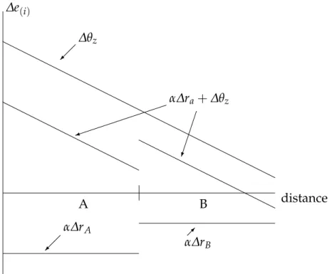
The easiest way to understand how the methodology works is to consider two neigh-bouring jurisdictions (A, B) where all sites are located on a straight line running through the two jurisdictions. With distance from the left hand end of jurisdiction A represented on the horizontal axis, figure 1 shows the change in the site specific effect at each location. Assume that the increase in the site-specific effect is highest for sites at the left hand end
A B distance ∆e(i) ∆θz α∆rA α∆rB α∆ra+∆θz )
Figure 1. Boundary discontinuities
of jurisdiction A and lowest at the right hand end of B. The line ∆θz shows the effect
on establishment employment at each location holding everything else equal. Everything else is not equal, however. Assume that jurisdictions base their tax increases on theaverage
change in site characteristics in their jurisdiction. Jurisdiction A sees larger increases in taxes than jurisdiction B. The impact on employment (again ceteris paribus) is shown as α∆ra. The overall employment effect is then represented by∆θz+α∆ra. Notice, that we
have assumed that the impact of site-specific effects tends to outweigh the increase in taxation, so thaton averageemployment growth in A is higher than in B. Thus, even after conditioning out establishment-specific effects, it appears that employment is positively related to taxes. Put differently, to estimate the effect of local taxation on employment one needs to condition out site-specific effects properly.
To do this, consider two sites on the border between A and B. By assumption, the establishments experience approximately the same site-specific effect. All else equal, their employment would grow by roughly the same amount. However, the establishment in
A sees a higher tax increase and this offsets the impact of the improved site. The overall effect on employment is given by α∆ra+∆θz which is larger for the establishment in B
than in A. The difference between the two isα(∆ra−∆rb). Since our procedure compares
the growth in employment in the establishment on the boundary in A to the growth in employment in the establishment on the boundary in B, we now correctly identify the negative relationship between increased taxation and employment. Of course, this ex-ample is just one possibility, but it does serve to emphasise exactly how our methodology allows us to correctly identify the impact of local taxes on employment.
Finally, before turning to the implementation, note that space differencing and the
within transformation have implications for the error structure. As usual, directly im-plementing (9) would yield consistent estimates for the coefficients but does not give the correct standard errors. Appendix A shows how to correct the standard errors when estimating (9).
To summarise, we use the panel dimension of our data to remove establishment and jurisdiction fixed effects. We then identify establishments with similar site-specific effects but that face different tax rates. These are establishments that are located close to one another but in different jurisdictions. We use these establishments to identify the impact of local taxation on employment. Later in the paper, we use similar ideas to consider the impact of local taxation on the entry of new establishments. As there are some differences in the implementation, we leave the details to section 5 and for now turn to outlining our data and the results for employment.
3. Data
To implement our methodology, our data needs to satisfy a number of requirements. First, we need to have a panel of individual establishment level data. Cross-sectional data do not allow us to use the within transformation to remove establishment and jurisdiction-specific effects. We then need to be able to precisely locate these establishments so that we can identify which pairs of establishments are neighbours. Finally, we need to identify
a local tax which is time-varying. We would prefer this local tax to be economically significant to increase the chances of detecting any impact on location and employment decisions. Data satisfying all of these requirements is available for England for the six year period from 1984 to 1989. We first describe the establishment level data set we use before turning to details of the particular local tax that we consider.
A. Establishment data
Our empirical analysis uses establishment level data for years 1984 to 1989 from the Annual Respondent Database (ARD) which is the data underlying the Annual Census of Production in the UK. Collected by the Office for National Statistics (ONS), the ARD is an extremely rich data set which contains information about all UK establishments from 1973 onwards. We face two restrictions on time period. Changes to the tax system restrict our focus to years before 1990, while changes to theARDrestrict us to years after 1983. We restrict ourselves to English manufacturing establishments.10 For every establishment, we know postcode, five-digit industrial classification, and number of employees. In our ana-lysis of employment we use only the information coming from a sub-sample of ‘selected’ establishments. These are the establishments that are requested to make a detailed return in any year. These establishments are generally larger and their employment information is of better quality than for non selected establishments.11 The precise sampling frame for selected establishments and further description of this data can be found in Griffith (1999). In our analysis of entry we use the exhaustive data (that includes ‘selected’ and ‘non-selected’ establishments).
The postcode reported in the ARD is very useful for locating establishments. In the UK, postcodes typically refer to one property or a very small group of dwellings. The CODE-POINT data set from the Ordnance Survey (OS) gives spatial coordinates (Eastings
10We ignore Scotland because it operated a different local tax system, Wales because it is not covered by
the data set that provides our instruments, and Northern Ireland because special permission is required to accessARDdata for establishments located there.
11The better quality of data is not the only reason to focus on selected establishments. Implementation of
the algorithm to identify neighbours and calculate data for pairs of neighbouring establishments is infeasible with the large samples that include non-selected establishments.
and Northings) for allUKpostcodes.12 By merging this data with theARDwe can generate very detailed information about the location of all English manufacturing establishments. For all but a tiny percentage of matched establishments the OSacknowledges a potential location error below 100 metres. For the remaining observations, the maximum error is a few kilometres. Overall, we expect a very high level of precision for our location data (see Duranton and Overman, 2005, for further discussion).
As the data requirements for our spatial differencing methodology are already some-what restrictive, we only consider establishment specific variables that can be calculated for all establishments. For the ARD, this means only controlling for establishment age. For establishments already in the panel in 1976 (the earliest year for which we have information), we are unable to assess their exact age. With our regressions running over 1984-1989, this truncation of the data implies that age is censored for establishments above 8 years in 1984. For consistency across years, we thus construct three age variables. One is a dummy for establishments that are 8 years or older. The other two are age and age squared defined only for establishments younger than 8 years old. The dummy captures the effect of being ‘old’ although it does not allow us to assess differences between old establishments and very old establishments. Age and its square for establishments less than 8 years old capture a non-linear effect of age for new establishments.
There are 25,579 establishments in theARD that are located in England and that report employment at least once within our study period. We make several sample restrictions. We deleted 122 establishments where the Local Authority code was missing since we need this to append the tax rate and political variables. We then dropped 374 establish-ments where we could not identify coordinates based on postcode as we cannot identify
neighbours for these establishments.13 A further 723 establishments change sector during the period and 2,547 move site (i.e., change coordinates). In both cases these changes frequently reflect coding errors rather than genuine changes in activity or location, so we drop these establishments. This leaves us with a sample of 21,813 establishments and a total of 61,785 observations.
B. Local taxation
The local tax that we consider is a property tax on non-residential property known as the UKbusiness rate, set and collected by jurisdictions called Local Authorities (hereafterLAs). Before 1990, tax rates varied over time and jurisdictions. We are fortunate because this tax consisted only of a flat rate that applied to all non-residential properties. This simplicity implies that the only source of variation is the tax rate itself.
TheUKbusiness rates were subject to a major reform in 1990 which essentially elimin-ated jurisdictional variation. This reform provides a large amount of exogenous variation in the tax rate. Unfortunately we cannot exploit it because all properties were also reval-ued in 1990. Since we do not know by how much each property was revalreval-ued, we cannot compute the change in taxation faced by each establishment. Hence, as mentioned above, while the production data restricts our study period to start in 1984, the reforms to the tax system mean it must end in 1989.
UK business rates are levied on the occupiers(not owners) of non-domestic properties according to the rental value of the property. These taxes represented a considerable tax on business. To give some idea of the economic significance of the tax, note that in 1990 the average annual rates bill per square foot was over £4, compared with an average rent bill per square foot of just over £13 (Bond, Denny, Hall, and McCluskey, 1996). Hence
13We directly identified Eastings and Northings for around 90% of establishments. The main problem for
the remaining 10% results from the creation of new postcodes not reported in our version of CODE-POINT. To increase matching rates, we checked our data against a data set of postcode updates. For observations with postcodes still unmatched, we imputed co-ordinates as follows. In theUK, a postcode is either six or seven digits. We first drop the last digit and assign establishments the mean coordinates of all postcodes sharing the same truncated postcode. If this failed to produce a match, we dropped two, then three digits from the postcode and again matched on mean coordinates where possible. This left us with a small percentage (1.4%) of establishments that could not be given a grid reference.
rates bills make up roughly 25 per cent of the total occupancy costs of rented commercial property. In 1992 business paid £13bn in local rates. A figure that was almost equal to the £15bn that they paid in corporation tax for the same year.
It is important to note that, as a first approximation, none of this money was used to finance local services for businesses. The responsibilities of LAs include social and health services for their residents, community safety, some aspects of education, housing, arts, culture, and environment. Nothing is directly provided to businesses.14 Even basic services such as refuse collection need to be separately organised by businesses.15 The only area of responsibility ofLAs that can affect businesses directly is planning (and some trading regulations that will affect mostly retail). Despite a mostly national set of planning regulations, LAs may differ in their speed of processing applications. It is hard to believe, however, that there were substantial within jurisdictional changes in the efficiency of local planning offices over the time period we consider. Instead, differences with respect to planning efficiency and restrictiveness, if they matter at all, are expected to be part of the fixed effect of these jurisdictions.
During our period of study, tax rates were set locally by the 366LAs in England, which entirely covered its land area. Large cities comprise several such LAs (e.g., 33 for London and 10 for Manchester). The tax paid depended on the value of the buildings occupied. The tax rates were known as ‘rate poundages’ and the value of the buildings as the ‘rateable value’. The tax rate was changed yearly. Rateable values of buildings were fixed in 1973 and did not change until 1990. The average rate for 1987 was 229.5 pence per pound of 1970 rateable value with a standard deviation of 32.2 pence. The ratio between the highest business rate (Oldham in Manchester) and the lowest (Kensington and Chelsea in London) was about three. These two LAs are of course far from each other and this
14Clearly, there may be some indirect effects through, for instance, crime or education. However we
expect these effects to spill over across jurisdictions so that establishments on both sides of any border face similar conditions. This argument is reinforced by the fact that LAs had only very limited autonomy on crime, because police districts usually comprise severalLAs.
15One of the key reasons why the Central government decided to take this tax setting power away from LAs in 1990 was that it acknowledged it was a taxation without representation nor services. Another reason
for this reform is that large increases in business rates suggested that UK LAs were engaged in something very much like a ‘race to the top’ rather than the often feared ‘race to the bottom’.
difference will not be taken into account in our estimation when we spatial difference. The largest ratio between two neighbouringLAs is nearly two. There was also significant time-series variation. There was for instance an average increase in the business rates of nearly 10 per cent between 1988 and 1989. Over the entire period (1984 −89) the average increase was 45 per cent with a standard deviation of 0.15. Again looking at neighbouringLAs, we observe a 25 per cent decrease in Kensington and Chelsea against a 31 percent increase in neighbouring Hammersmith over the period. We think this is more than sufficient variation to perform our estimations.
4. Results
We use log employment (eit) as the dependent variable. As explanatory variables we include log tax rate (rat), the three variables described above to capture the impact of
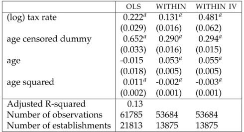
age (Xit) and a full set of industry-year dummies (two-digit industries) for which we do not report coefficients. To show the difference that our estimation strategy makes, we also estimate the effects of local taxation using standard techniques. Results for the non-spatial specifications (i.e., using standard techniques and ignoring the micro-spatial nature of the data) are reported in table 1. Table 2 reports results for comparable specifications that use spatial differencing. For the sake of comparison, we have restricted the sample to be the same for all specifications by only including those establishments that we use to estimate our preferred specification: the instrumented, fixed effect spatial-differencing specification discussed below (the final specification in table 2). This restriction requires establishments to be in a pair in which both establishments simultaneously report em-ployment in at least two years.16
16Consider an establishment that reports employment for (say) only 1987 and 1988. It is in the sample if it
has at least one neighbour and that neighbour also reports employment for these two years. It is not in the sample if it has no neighbours or if it has neighbours but they do not also report employment in 1987 and 1988. We impose this restriction because our implementation of spatial-differencing uses fixed effects for pairs, rather than estimating the fixed effect for establishments and then spatial differencing. Furthermore, an establishment can be part of more than one pair satisfying this condition. However, we only use each establishment once in estimating the non-spatial specifications.
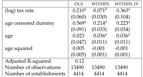
OLS WITHIN WITHIN IV (log) tax rate 0.210a 0.071b 0.363a
(0.060) (0.030) (0.104) age censored dummy 0.569a 0.214a 0.223a (0.091) (0.033) (0.034) age 0.023 0.036a 0.036a (0.047) (0.011) (0.011) age squared 0.005 -0.001 -0.001 (0.005) (0.001) (0.001) Adjusted R-squared 0.12 Number of observations 13490 13490 13490 Number of establishments 4414 4414 4414
Notes: Regression of (log) employment on (log) local tax rates and age variables. First column reports results from OLS, second column (WITHIN)
allows for establishment specific fixed effects, third column (WITHIN IV)
further instruments local tax using local political variables. Standard errors under coefficients. a,bandcdenote significance at the 1%, 5% and 10% level respectively.
Table 1. Non-spatial regression results
Starting with 21,813 establishments, 7,938 of them are dropped because they only report employment once, independently of whether they are in a pair. Of the remaining 13,875 establishments, 8,792 have a neighbour within 1 kilometre (the distance threshold that we use for our reported results). However, only 4,414 of these establishments are in at least one pair where both establishments simultaneously report employment in at least two years. These establishments form the restricted sample for which we report results in the text. To show that this sample is representative, Appendix B reports results for the same specifications but without imposing this sample restriction.
The first regression in table 1 reports the results from estimating equation (5) using pooled OLS for all six years 1984-1989. The results on the age variables show that, as expected, older establishments have higher employment. Our main focus, however, is on the role of taxation and from our results we see that in the cross-section, higher tax rates are associated with higher employment.
As we noted above in our discussion of equation (5), one possible explanation of this positive correlation is that some establishments are larger than others for unobserved reasons and larger establishments happen to be located in higher tax jurisdictions. The
second specification in table 1 allows for this possibility by introducing an establishment-specific fixed effect and calculating thewithinestimator. From the table we can see that the coefficient on tax rate is divided by three suggesting that much of the positive correlation between employment and local tax rate is indeed due to unobserved characteristics of establishments. Note, however, that the effect remains positive and significant.
The remaining problem that we need to tackle is that the tax rate may be correlated with the error in equation (6). There are two possible sources for this correlation. First, there may be a feedback from local employment to local tax rate. This feedback will be positive when local politicians feel able to tax local business more when it is doing well. Alternatively, and working in the opposite direction, it could be that LAs can afford to keep taxes low during ’good times’. In the UK context, this alternative may arise because some redistribution takes place locally so that good times may imply a lesser need for social expenditure. This being said, we do expect the first effect to dominate and taxation to go up when local business is doing well. Second, there may be other time-varying characteristics that are positively correlated with both employment and tax rates and that we do not control for through the use of establishment-specific fixed effects. Recall that the establishment fixed effects only condition out time-invariant unobserved heterogeneity.
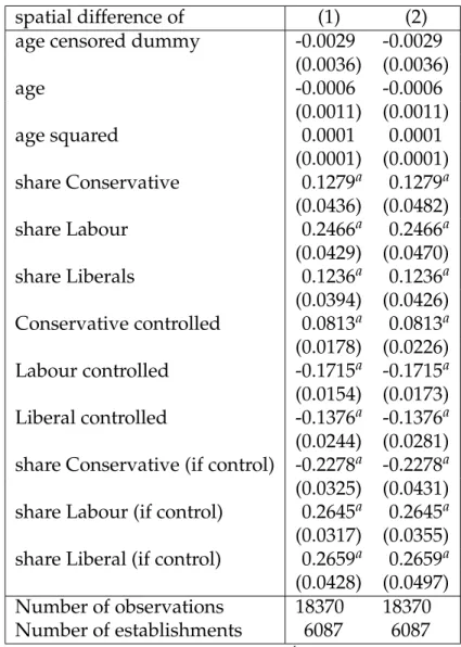
To solve these problems we take an instrumental variable approach. More specifically, we use local political variables to instrument for local tax rates.17 The full set of instru-ments includes the share of local politicians affiliated with the Conservative, Labour and Liberal Democrat parties, a set of dummies indicating whether the LA is controlled by the Conservative, Labour or Liberals and a set of interactions giving the share of the Conservatives, Labour and Liberals if they control the LA.18 The R-squared of the first stage regression is 69%. For the interested reader Appendix C provides further details on
17The data is from the British Local Election Database which is available through theUKData Archive. 18These are the three main political parties. There are many smaller parties that play a role in local politics
the first stage regression.19
The third column in table 1 shows what happens when we use these instruments for the level of taxation in the fixed effects specification that we reported in column 2. Sur-prisingly, perhaps, the coefficient on local taxation actually increases after instrumenting. It would be tempting to conclude that, contrary to most priors, UK LAs taxed businesses according to jurisdictions (social) needs rather than local business’ capacity to pay. That is, there is a negative correlation between local tax rates and the omitted variables so that instrumenting leads to a higher coefficient on local taxation. Nonetheless, a positive effect of local taxation on employment with an elasticity close to 0.4 strikes us as implausible. As we will see below it appears that this increase in the coefficient on local taxation following instrumentation occurs because the unobserved time-varying site-specific effect is correlated with both employment and local political variables.20
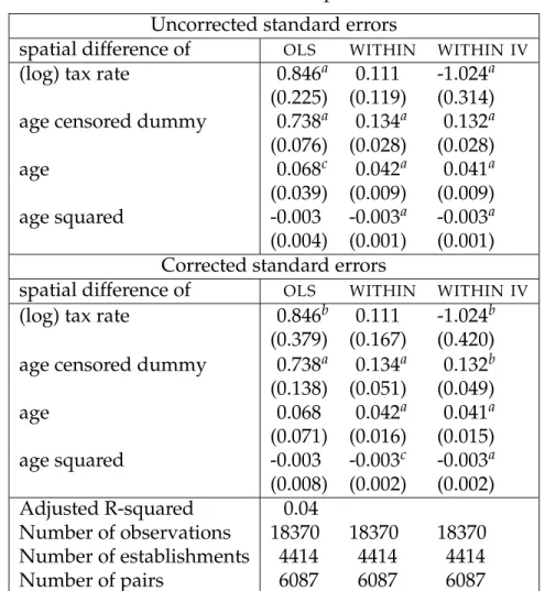
In table 2 we present two sets of results (with and without corrected standard errors) for three different spatial specifications that parallel those presented in table 1. In the first column, we spatial difference equation (5) and then estimate it using OLS. In the second, we spatial difference (6) and then estimate it using a fixed effect for each pair of establishments.21 Finally in the third column, we instrument the tax rate in the spatially differencedwithinspecification using spatially differenced political variables as in the non-spatial specification.
The results that we report use a distance threshold of 1 kilometre to identify neighbours. In our choice of threshold, we face a tradeoff between sample size and the extent to which the spatially varying site-specific effects are equal across neighbouring sites. We chose the minimum threshold which gives us sufficient observations to identify the effect of local
19One might be tempted to test for the validity of instruments given that we have more instruments than
endogenous regressors. We would argue, however, that such a test is invalid because all our instruments are based on the same underlying assumption (that local politics is independent of changes to establishments’ employment).
20One possible solution would be to use lagged values of the political variables as instruments. However,
this would mean dropping years from a short panel and would only solve the problem if there is no correlation in the unobserved factors and the political variables over time. Instead, we use our spatial differencing strategy to control for these unobserved time-varying effects.
21Our pairing algorithm only matches establishments if they are in the same 2 digit sic, so we do not need
taxes (remembering that the identification of the tax effect comes from cross jurisdiction border pairs). We use neighbouring establishments within the same jurisdiction to im-prove our estimates of the effect of establishment-specific variables.22
Uncorrected standard errors
spatial difference of OLS WITHIN WITHIN IV (log) tax rate 0.846a 0.111 -1.024a
(0.225) (0.119) (0.314) age censored dummy 0.738a 0.134a 0.132a (0.076) (0.028) (0.028) age 0.068c 0.042a 0.041a (0.039) (0.009) (0.009) age squared -0.003 -0.003a -0.003a (0.004) (0.001) (0.001) Corrected standard errors
spatial difference of OLS WITHIN WITHIN IV (log) tax rate 0.846b 0.111 -1.024b
(0.379) (0.167) (0.420) age censored dummy 0.738a 0.134a 0.132b (0.138) (0.051) (0.049) age 0.068 0.042a 0.041a (0.071) (0.016) (0.015) age squared -0.003 -0.003c -0.003a (0.008) (0.002) (0.002) Adjusted R-squared 0.04 Number of observations 18370 18370 18370 Number of establishments 4414 4414 4414 Number of pairs 6087 6087 6087
Notes: Regression of spatial difference of (log) employment on spatial difference of (log) local tax rates and age variables. First column reports results fromOLS, second column (WITHIN) allows for establishment specific fixed effects, third column (WITHIN IV) further instruments local tax using local political variables. Standard errors under coefficients. First block of results report uncorrected standard errors. Second block of results report standard errors corrected according to Appendix A. a, b and c denote significance at the 1%, 5% and 10% level respectively.
Table 2. Spatial differencing regression results
Note that, although the overall sample of establishments is restricted to be identical for both the spatial and non-spatial specifications, the number of observations is higher for the spatially differenced specifications (18,370 compared to 13,490). This is because each
22We get the same results if we restrict attention only to the 164 establishments that are part of
cross-jurisdiction border pairs. The spatially differenced withinIV specification gives a coefficient of −1.072 as opposed to the−1.024 reported in the text. Both coefficients are significant at the 1% level.
establishment can be involved in more than one pair. Specifically, we have 6,087 unique pairs as compared to 4,414 unique establishments suggesting that each establishment has on average three neighbours.23
Before turning to the individual coefficients, comparing the two blocks of results (with and without corrected standard errors), we see the corrections outlined in Appendix A generally increases estimates of standard errors by around 50%. In our particular context, this results in some minor changes in significance levels, but does not change our overall findings. In other contexts it clearly could, suggesting that the correction outlined in the appendix should usually be implemented. Turning to the coefficients, we see that, apart from changes in significance levels, the results on the age variables are essentially unchanged. As before, we focus on the impact of the local tax rate and note that after spatial differencing we get a higher correlation between (spatially differenced) local tax rate and (spatially differenced) employment than previously, with a coefficient of 0.846 compared to 0.210 with OLS. These coefficients have the same probability limit when there are no unobserved establishment or site-specific effects, or when these effects are uncorrelated with tax rates or other included explanatory variables. A possible reason for the higher correlation between employment and taxation after controlling out site-specific effects is that areas with poor sites had higher local tax rates thus biasing downward the coefficient on local taxes in the non-spatial OLS estimation which ignores these local site-specific effects. A correlation between having ’poor sites’ (following bad local economic conditions during the period) and higher taxes is certainly believable given the political economy of UK LAs: de-industrialisingLAs tended to vote for very left-wing councils that then greatly increased local taxation.24
However, this interpretation is based on the assumption that establishment fixed effects are either absent or uncorrelated with local tax rates. To account for the possible
correl-23Working against this, is the fact that both establishments in the pair must simultaneously report
em-ployment data in at least two years. For this distance threshold the first effect dominates. That need not be the case for other distance thresholds.
24For instance, Sheffield council under the leadership of the (then) leftwing firebrand David Blunkett
ended up with the highest business rate in the country in 1990 and Liverpool council led by the equally notorious Derek Hatton ranked 12th.
ation between establishment fixed effects and local tax rates we use, as before, the panel dimension of our data. This controls for unobserved establishment heterogeneity. We do that in the column 2 of table 2 which reports results when we both spatially difference and allow for fixed effects for pairs of establishments. Note that these pair fixed effects not only control for time-invariant unobserved establishment heterogeneity but also for other time-invariant local effects such as the (possible though unlikely) propensity of some jurisdictions to provide better services and thus have consistently better performing establishments.
Comparing results across the non-spatial and spatially differenced specifications we see that after controlling for establishments fixed effects, the coefficient on local tax rate is again higher after we spatial difference. However because of higher standard errors, it is hard to provide a definitive interpretation for this comparison. More significantly, comparing across the spatially differenced specifications, we see that allowing for pair fixed effects reduces our estimate of the positive correlation between local taxation and employment relative to the spatially differencedOLSresults. The coefficient even becomes insignificant. This confirms our finding from the non-spatial specifications that estab-lishment fixed effects appear to be positively correlated with tax rates: LAs with ‘good’ establishments charge higher taxes.
As with the non-spatial fixed effects specifications, we still want to control for the fact that local tax rates may be endogenous. To do this, we instrument using the spatial difference of the same set of political variables that we use for the non-spatial specification. Results are shown in column 3 of table 2. We now see that local taxation has a negative effect on establishment employment. As argued above, the difference between the spatial and non-spatial results suggests that the unobserved time-varying site specific effects are correlated with both employment and local political variables. Spatial differencing re-moves these site-specific effects, ensuring that our instruments are valid and thus allowing us to identify the negative effect of local taxes on establishment employment.
over existing methodologies. First, comparing the instrumented spatial and non-spatial regressions allows us to identify the nature of the relationship between site-specific effects and local taxation. Second, and more importantly, because spatial differencing removes unobserved time-varying site-specific effects it makes it far easier to find a valid set of instruments that allows us to identify the negative relationship between local tax-ation and employment. Quantitatively, spatial differencing greatly affects the results. In what is arguably the best estimation using standard techniques (again one that does not control for time-varying site-specific effects), we find a positive elasticity around 0.4. Our preferred specification with spatial differencing reverses the sign of the coefficient and leads to an elasticity around−1 (although it is not very precisely estimated). In a nutshell, instead of a positive effect of local taxation on employment, we find, thanks to our spatial differencing approach, a significant negative effect of local taxation on local employment. The negative effect of local taxation on employment is possibly stronger than one would have thought since this tax is not far from an ideal land tax. There are, however, two differences with a non-distortionary land tax. The first is that building extensions were taxed. This could have had an especially important effect because expansions would typically lead to a complete building re-assessment with the risk of an increase in taxation on the already existing facilities as well as the new ones. The second distortion is more subtle. It finds its root in the reciprocal hold-up problem which occurs because most manufacturing facilities are fairly specific to their tenant and conversely. With a vast majority of manufacturing firms renting their facilities, this hold-up problem is mitigated in UK manufacturing by having long-term rental contracts (typically 20 years) that are renegotiated only every five years or so. These long lags between rent negotiations probably meant that tax increases would not capitalise very fast and thus fall primarily on the (mobile) occupier who had to pay them. We believe that both these distortions help explain our finding of a negative effect of local taxation on employment.
5. Entries
A. Methodology and data
We now turn to the effects of local taxation on entry decisions. This is an important issue for two reasons. First, the rate at which new establishments enter LAs is an important economic outcome that deserves specific attention. Second, spatial differencing provides solutions to the same three problems (establishment heterogeneity, site heterogeneity, and endogeneity) that we addressed when looking at employment growth. However, there are subtle differences which we believe are worth highlighting.
Consider establishmentithat wishes to enter in yeart. It can choose between all avail-able sites, indexed by z. As before, the jurisdiction that sets the tax for the establishment depends on the site occupied, and is indexed bya. Profit maximisation can be performed in two stages. First, establishmenticomputes the highest profit it can achieve,Πiz, at each sitez. It then selects the site offering the highest profit.25 We assume that the highest profit for establishmentientering in yeartat sitezcan be written as:
Πizt =λrat+Zitζ+νi+κa+ϕzt+ǫizt (10)
whereνiis an establishment fixed effect,κais a jurisdiction fixed effect,Zitare explanatory
variables at the establishment level, ϕztis a site-specific effect, andǫiztis an establishment
site-specific shock.26 Establishmentiwill choose the sitezthat gives the highest expected profit. When the shocks ǫiz follow an appropriate iid extreme value distribution, the probability of choosing sitez, Pizt, is logistic and is given by
Pizt = expE(Πizt)
∑Zz=1expE(Πizt) (11)
25We ignore any possible interaction between the location decisions of entrants. Constraints on site choices
aside, this seems reasonable in established manufacturing industries where existing establishments drive local wages, determine product market competition etc. As discussed in the text, the fact that the effect on profits of these factors will be highly correlated across neighbouring sites then justifies our approach.
26The establishment fixed effect, ν
i, mirrors µi in (5). Similarly the jurisdiction effect, κa, and the
site-specific effect, ϕzt, are the counterparts ofγaandθzt. Finally both (10) and (5) contain coefficients for the
effect of local taxation (λandα) and establishment-level variables (ζand β). Note that our approach for entries is also consistent with a more general setting where the specification includes variables that are individual-site specific,φizt, in addition to individual effects,νi, and site effects,ϕzt.
where E(·)is the expectation operator and the summation is across all possible sitesZ. The standard approach to estimating the coefficients on tax rate and establishment spe-cific variables (λandζ) is to ignore the site-specific effect, ϕzt, and estimate a conditional
logit model. To do this, one creates a set of establishment-jurisdiction observations and defines cia = 1 if establishment i locates in jurisdiction a and cia = 0 otherwise. The coefficients can then be estimated by maximising the log likelihood of the conditional logit model: logLcl = I
∑
i=1 A∑
a=1 cia logPia (12)where for simplicity we have dropped the time subscripts as establishments only enter once.
As is well recognised in the literature, application of the conditional logit model can be problematic when the set of possible jurisdictions is large. One possible solution is then to take a random sub-sample of jurisdictions, although this clearly has implications for the efficiency of the estimator and the small sample properties are unknown. Another possibility, recently proposed by Guimaraes, Figueiredo, and Woodward (2003) is to use the fact that, under certain conditions, the log likelihood of the Poisson model is identical to that of the conditional log likelihood. Estimating a Poisson regression is computa-tionally much easier though the equivalence between the likelihoods only holds in the absence of establishment specific variables (i.e., Zit).27 In any case both solutions ignore the site-specific effects. As we now show, spatial differencing provides an alternative which controls for site-specific effects and which, in other contexts, would allow for the inclusion of establishment specific variables.
Our approach is as follows. Consider two neighbouring sites close to the border between two jurisdictions a1anda2. One site, denotedz1, is located in jurisdictiona1. The other, z2, is located in jurisdiction a2. Since the two locations are very close, we assume that ϕz1t ≈ ϕz2t. This is the same identification assumption made in section 2 to derive
our employment specification (9). To repeat, this assumption is justified by the fact that
27Guimaraeset al. (2003) show that the Poisson regression can also be used to simplify computation in
site-specific effects (labour market conditions, access to markets and major facilities, etc) vary smoothly across space. The probability of choosingz1conditional on locating in one of these two neighbouring sites is:
P(i∈ z1|i∈ {z1,z2}) = Piz1
Piz1 +Piz2
(13) Note that unlike equation (11) above, this specification conditions out both establishment-and site-specific effects. This occurs because these effects are the same at both locationsz1
and z2.28 In relation to this, recall that in standard conditional logit models observed site-specific factors are computationally hard to deal with. By contrast our approach directly conditions out both observed and unobserved site-specific factors in a way that is computationally easy to implement. In addition, we do not need to rely on the assump-tion of the Independence of Irrelevant Alternatives which underlies the condiassump-tional logit model. This is a distinct advantage as it is often argued that this assumption is unlikely to hold in spatial settings (see, for example, Head and Mayer, 2004).
When the shocksǫizt follow an appropriateiidextreme value distribution, the probab-ility of choosing one of the sites is logistic and is given by:
P(i ∈ z1|i ∈ {z1,z2}) = 1
1+exp(λ(ra2t−ra1t) +κa2 −κa1)
(14) In our particular application, equation (14) only involves jurisdictional level variables so we can estimateλdirectly from an aggregate logit model where the observation units are the (border-side, time) pairs. In the estimation, the observations are weighted by the number of entrants for consistency with equation (14).
In a nutshell, we select entrants located close to jurisdictional boundaries and examine their decision to choose to locate on one particular side of the border. The main conceptual difference with our employment regression (9) is that we consider the location decision of a new establishment choosing between neighbouring jurisdictionsrather than comparing
28We assumed in (10) that the effect of establishment characteristics did not depend on location. However
our spatial differentiation approach is more powerful than this since any interaction between establishment and site characteristics is conditioned out by spatial differencing provided the characteristics of the local environment vary smoothly over space.
the employment outcomes for (existing) neighbouring establishments. For entry, this is the appropriate way to control for both time invariant establishment specific effects and any unobserved site-specific effects common to both sides of a border.29 As local tax rates do not vary smoothly across space at jurisdictional boundaries, we can use entrants on either side of these boundaries to identify the effect of taxes after conditioning out time-varying site-specific factors and time-invariant establishment-specific effects. In-terestingly one step is enough to eliminate both establishment and site effects for entry, whereas two steps are necessary when studying employment. This reflects the fact that instead of comparing each establishment with a matched establishment on the other side of the border we compare each establishment with itself on the two sides of the border making thewithintransformation redundant.
As with the employment specifications, endogeneity must also be addressed since the local rate of taxation may be simultaneously determined with the rate of entry. To control for this, we estimate a two-stage IV logit model instrumenting the difference in tax rate,
ra2t −ra1t, in the logit specification, with the predicted difference in tax rate from a first
stage regression using spatially-differenced local political variables. The simplicity of this method comes at a price because, as is well known, correcting the errors to allow for possible correlation between the residual of the instrumentation equation and that of the entry equation is far from straightforward.30
B. Results
To construct the entry data, we need to detect all entrants in theARD. Because of a change in 1984 in the way the registry of establishments was constructed, there is a large amount of artificial entry in 1984 and 1985 (i.e., establishments enter the data set for the first time
29To see this, note that when choosing between two neighbouring sites, the entrant compares profits
between them. Time-varying site-specific factors, which vary smoothly across space, will affect profits at both sites in the same way. Hence, these factors do not enter into the location decision. A similar argument applies to unobserved time-invariant establishment characteristics.
30As an alternative, we used an IV probitmodel that estimates the entry and instrumenting equation
simultaneously. This approach provides us with the correct standard errors but at the cost that it is not fully consistent with the theoretical specification. The results are the same as with the two-stagelogitmodel.
during those two years even though they already existed prior to 1984). See Griffith (1999) for further discussion. As a result, we ignore entries for these two years and focus instead on all newly reporting establishments between 1986 and 1989. There are 81,042 entrants between 1986 and 1989.
For consistency with the employment regressions we would like to identify all entrants within 1 kilometre either side of jurisdiction boundaries. The easiest way to do this would be to draw 1 kilometre buffers around boundaries. Lacking a set of digital boundaries for this time period, we instead proceed indirectly and identify the set of border entrants from theARD itself. To do this, for each entrant we searched for the closest establishment located in each of the neighbouringLAs and retained only those entrants that had such a neighbour within one kilometre. Since this detection procedure is only meant to compute distances to the LA border for each entrant (rather than find a match for a pair), we considered all possible establishments in all sectors and all years as potential neighbours. We expect this procedure to catch nearly all entrants that are located within one kilometre of a border.
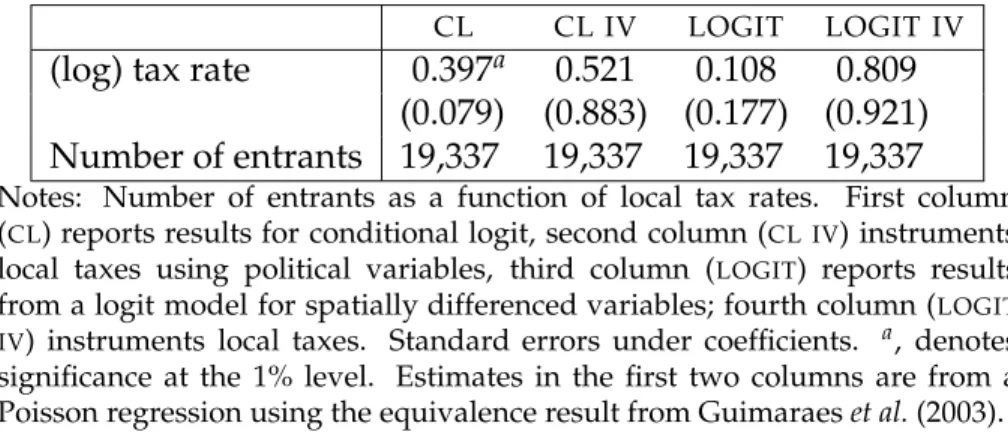
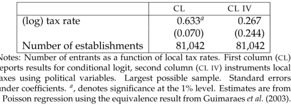
As for employment, we implement both the standard methodology (i.e., conditional logit) and our spatial differencing approach. Results for two non-spatial specifications, are given in columns 1 and 2 of table 3 while columns 3 and 4 report results for two comparable spatial specifications. Again, for the sake of comparison, we have restricted the sample to be the same for all specifications. This restriction requires establishments to locate within 1 kilometre of a boundary between two English LAs between 1986 and 1989. Imposing this requirement leaves us with a sample of 19,337 establishments. To show that this sample is representative, Appendix B once again reports results for the same specifications but without imposing this restriction.
Starting with the conditional logit we see, from the results reported in column 1, that there appears to be a positive effect of tax rates on entry. As discussed above this positive relationship may be driven by endogeneity. Column 2 shows what happens when we cor-rect for this by replacing the actual tax rates with the predicted tax rates from a first stage
CL CL IV LOGIT LOGIT IV (log) tax rate 0.397a 0.521 0.108 0.809
(0.079) (0.883) (0.177) (0.921) Number of entrants 19,337 19,337 19,337 19,337 Notes: Number of entrants as a function of local tax rates. First column (CL) reports results for conditional logit, second column (CL IV) instruments local taxes using political variables, third column (LOGIT) reports results from a logit model for spatially differenced variables; fourth column (LOGIT IV) instruments local taxes. Standard errors under coefficients. a, denotes significance at the 1% level. Estimates in the first two columns are from a Poisson regression using the equivalence result from Guimaraeset al.(2003).
Table 3. Results for entries
regression of tax rates on political variables. Once instrumenting, we find no significant relationship between tax rates and entry. Correcting the standard errors to allow for the fact that we are instrumenting would only reinforce this finding.31 Columns 3 and 4 show that we reach exactly the same conclusions on the irrelevance of tax rates for entry using our spatially differenced approach.
This lack of effect of local taxation on entry is consistent with the interpretation we gave above for our employment results. Recall that the negative effect of local taxation on firm growth was attributed to imperfect capitalisation of the local tax rate into property rental prices. In turn, imperfect capitalisation was attributed to the imperfect mobility of existing firms and the lags between rent negotiations. Unlike existing firms, new entrants are mobile and negotiate their rents upon entry so that the capitalisation of local taxation is expected to be near perfect. In such case, the burden of local taxation should fall only on the landlords and leave the behaviour of firms undistorted.
6. Conclusion
We propose a new approach to assess the effects of local taxation. Our results point to the importance of controlling for both unobserved establishment-specific and unob-served site-specific characteristics and possible simultaneity. Simple OLS results
sug-31Hence our decision only to implement the theoretically consistent two stage conditional logit procedure
gest a positive relationship between employment and taxes. Allowing for unobserved establishment-specific effects and instrumenting for local taxation, we still find a positive relationship between employment and taxes. Allowing for unobserved location-specific effects and instrumenting for local taxation, we find a negative significant relationship between employment and taxes. By contrast we find that local taxation has no effect on the entry of new establishments.
Beyond our methodological contribution, this analysis also suggests that the study of local taxation and, more broadly, that of decentralised public intervention faces serious endogeneity problems whereby local public decisions depend strongly on very local con-ditions, which are extremely difficult to control for. As shown here, properly controlling for such local conditions is a necessary condition to obtain reliable estimates.
The second broad lesson is that even taxes that are seemingly close to an ‘ideal’ tax that would be free of distortion can in practice generate significant distortions. Despite the fact that the UKbusiness rates were close to George’s 1884 ’pure’ land tax, frictions in the rental market implied that increases in local taxation were not fully capitalised into the rents and thus had an adverse effect on employment.