Research Online
Research Online
University of Wollongong Thesis Collection
1954-2016 University of Wollongong Thesis Collections
2016
Pricing American-style Parisian options
Pricing American-style Parisian options
Tan Nhat Le
University of Wollongong, [email protected]
Follow this and additional works at: https://ro.uow.edu.au/theses
University of Wollongong University of Wollongong
Copyright Warning Copyright Warning
You may print or download ONE copy of this document for the purpose of your own research or study. The University does not authorise you to copy, communicate or otherwise make available electronically to any other person any
copyright material contained on this site.
You are reminded of the following: This work is copyright. Apart from any use permitted under the Copyright Act 1968, no part of this work may be reproduced by any process, nor may any other exclusive right be exercised, without the permission of the author. Copyright owners are entitled to take legal action against persons who infringe
their copyright. A reproduction of material that is protected by copyright may be a copyright infringement. A court may impose penalties and award damages in relation to offences and infringements relating to copyright material.
Higher penalties may apply, and higher damages may be awarded, for offences and infringements involving the conversion of material into digital or electronic form.
Unless otherwise indicated, the views expressed in this thesis are those of the author and do not necessarily Unless otherwise indicated, the views expressed in this thesis are those of the author and do not necessarily represent the views of the University of Wollongong.
represent the views of the University of Wollongong. Recommended Citation
Recommended Citation
Le, Tan Nhat, Pricing American-style Parisian options, Doctor of Philosophy thesis, School of
Mathematics and Applied Statistics, University of Wollongong, 2016. https://ro.uow.edu.au/theses/4654
Research Online is the open access institutional repository for the University of Wollongong. For further information contact the UOW Library: [email protected]
A thesis submitted in fulfilment of the requirements for the award of the degree
Doctor of Philosophy
fromUniversity of Wollongong
by LENhat TanI,LE Nhat Tan, declare that this thesis, submitted in partial fulfilment of the requirements for the award of Doctor of Philosophy, in the School of Mathematics and Applied Statistics, University of Wollongong, is wholly my own work unless otherwise referenced or acknowledged. The document has not been submitted for qualifications at any other academic institution.
LE Nhat Tan
Barrier options are the most common path-dependent options traded in financial markets. They are particularly attractive to investors, because not only are they cheaper than vanilla options but they also offer different choices of investment, which allow investors to bet their views on the movement of the underlying asset prices. The “one-touch” breaching barrier however is prone to market manipulations which can be made by influential agents in order to free them from their liabilities to the option holders. Aiming to prevent such market ma-nipulations, Parisian options were introduced, with an extended trigger clause, which makes the knock-in or knock-out feature much harder to be activated. Pricing Parisian options has become an increasingly important problem from both financial and mathematical per-spectives. Financially, the introduction of Parisian options, which makes the market fairer in the sense that it protects the holder of Parisian options from deliberate action taken by the writer, requires an efficient way to precisely evaluate the option prices. On the other hand, due to the presence of the newly-added trigger clause, the valuation of Parisian op-tions becomes a three-dimensional problem, a challenging problem, which has hindered the application of various mathematical methods. In this thesis, we explore the integral equation method and the “moving window” technique to price different types of Parisian options under the Black-Scholes framework.
Firstly, we price an American-style down-and-out call, which can be considered as a spe-cial Parisian option with zero “option window”. Instead of using the probability theory as used in the literature, we use the continuous Fourier sine transform to solve the partial dif-ferential equation system governing the option price. As a way of validating our approach, we show that the “early exercise premium representation” for American-style down-and-out calls without rebate can be re-derived by using our approach. We then examine the case that time-dependent rebates are included in the contract of American-style down-and-out calls. As a result, a more general integral representation for the price of an American-style down-and-out call, with the presence of an extra term associated with the rebate, can be obtained. Our numerical method based on the newly-derived integral representation appears to be efficient
in computing the price and the hedging parameters for American-style down-and-out calls with rebates. In addition, significant effects of rebates on the option prices and the optimal exercise boundaries are illustrated through selected numerical results.
Secondly, in Chapters 4 and 5, we price two different types of American-style Parisian knock-in call options: up-type and down-type, respectively. Usually, pricing an American-style option is much more difficult than pricing its European-American-style counterpart because of the appearance of the optimal exercise boundary in the former. Fortunately, the optimal exercise boundary associated with an American-style Parisian knock-in option only appears
implicitly in its pricing partial differential equation systems, instead ofexplicitly as in the case of an American-style Parisian knock-out option. As a result, the “moving window” technique developed for pricing European-style Parisian knock-out call options can be adopted to price American-style Parisian knock-in options as well. In particular, we have obtained simple analytical solutions for American-style Parisian knock-in call options, which can be easily computed numerically.
Thirdly, in Chapters 6 and 7, we propose an integral equation approach for pricing two different types of American-style Parisian knock-out call options: up-type and down-type, respectively. The corresponding three-dimensional pricing problem is first reduced to solv-ing a pair of coupled two-dimensional partial differential equations by applysolv-ing the “movsolv-ing window” technique. The newly-derived two-dimensional systems are then analytically solved separately as if they were not coupled. As a result, we can obtain integral representations for the option prices at any asset price, in terms of unknown quantities: the option prices at the asset barrier and the optimal exercise prices. These unknown quantities are in turn governed by a pair of coupled integral equations, which can be efficiently solved by using the Newton-Raphson iterative procedure. Consequently, the option prices and the hedging parameters can be obtained both accurately and efficiently. Numerical results are also examined in or-der to provide new insight into interesting features about prices of American-style Parisian knock-out call options and the behavior of the associated optimal exercise boundaries.
Finally, in the last chapter, we briefly summarize the main results achieved in this thesis and propose future research directions to extend these results.
First and foremost, I would like to sincerely thank my principal supervisor, Prof. Song-Ping Zhu, for his insightful supervision and substantial advice during my doctoral study. I, in particular, appreciate him for introducing me into financial mathematics, a very interesting research area. His high professional standard and rigorous attitude towards research have exceptionally inspired and transformed me from a raw beginner to a potential researcher. I am indebted to him more than what I can say.
To my dear co-supervisor, Dr. Xiaoping Lu, I am truly thankful for her guidance, encour-agement and warm care throughout the research. She is always patient and gives me abundant time to have consultation. My thanks also go to Dr. Wenting Chen, my former co-supervisor, for being such an excellent example of a highly successful early career researcher, which I wish to be in the near future.
My deep appreciation goes to Dr. Nguyen An Khuong for encouraging me to study abroad and getting me started on my research journey. Needless to say, I am extremely grateful for financial support from the Australian government, who have provided me an AusAID scholarship to pursue my dream of being an academic researcher.
To all my mathematics teachers at Le Loi high school and Quy Nhon university, you all have helped me to fall in love with mathematics, for that I am truly grateful. My thanks also go to my friends at English conversation group and Vietnamese dynamic society in Wollongong, you have been a great support network to me.
Words actually fail to express my appreciation to my parents, Mr. Dinh and Ms. Thu, for their endless support, encouragement and love. Thank you for educating me to be a good person and always supporting me to pursue my dream. I would also like to thank my beautiful and intelligent wife, Ms. Tram, for her dedication, love and persistent confidence in me.
1 Introduction 1
1.1 Options and option pricing problems . . . 1
1.2 Literature review . . . 2 1.2.1 Vanilla options . . . 2 1.2.2 Barrier options . . . 5 1.2.3 Parisian options . . . 7 1.3 Structure of Thesis . . . 10 2 Theoretical background 12 2.1 Asset price dynamics and stochastic processes . . . 12
2.2 The Black-Scholes model . . . 15
2.2.1 The Black-Scholes equation . . . 15
2.2.2 The governing PDE system . . . 17
2.2.3 Initial-value heat problem in the infinite domain . . . 18
2.2.4 The Black-Scholes formula . . . 20
2.3 The integral representation of American vanilla options . . . 21
2.4 Integral equations . . . 29
2.5 Pricing European barrier options . . . 37
2.5.1 Formulation . . . 37
2.5.2 Initial-value heat problem in a semi-infinite domain . . . 39
2.5.3 A closed-form solution of European down-and-out calls options . . . 41
3 Pricing American-style down-and-out calls with rebates 43
3.1 Introduction . . . 43
3.2 The governing PDE system . . . 45
3.3 Our analytical solution procedure . . . 46
3.3.1 Applying the Fourier sine transform . . . 47
3.3.2 Inverting the Fourier sine transform . . . 50
3.3.3 Integral representation . . . 53
3.3.4 Hedging parameters . . . 55
3.4 Numerical implementation . . . 59
3.4.1 The optimal exercise boundary just prior to expiry . . . 59
3.4.2 Numerical procedure . . . 62
3.5 Numerical results . . . 63
3.5.1 Validation of our numerical scheme . . . 63
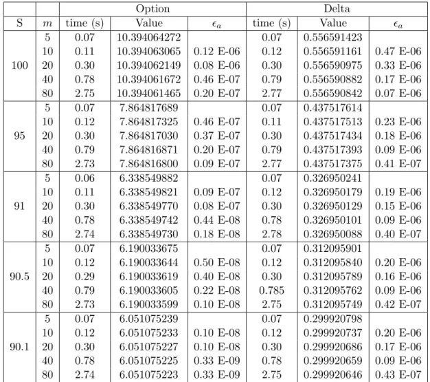
3.5.2 The accuracy and efficiency of our numerical scheme . . . 64
3.5.3 Effects of rebates on the optimal exercise price . . . 66
3.5.4 Effects of rebates on the option price . . . 68
3.6 Conclusion . . . 72
4 Pricing American-style Parisian up-and-in options 73 4.1 Introduction . . . 73
4.2 Formulation . . . 75
4.3 Solution procedure . . . 77
4.4 Numerical example and discussion . . . 84
4.5 Conclusion . . . 87
5 Pricing American-style Parisian down-and-in options 88 5.1 Introduction . . . 88
5.2 The PDE systems . . . 89
5.3 Solution of the coupled PDE systems . . . 90
5.4 Numerical example and discussion . . . 94
6 Pricing American-style Parisian up-and-out call options 97
6.1 Introduction . . . 97
6.2 Formulation . . . 99
6.3 Our solution procedure . . . 107
6.3.1 The dimensionless heat systems . . . 108
6.3.2 Integral representations of the option prices . . . 110
6.3.3 Coupled integral equations . . . 112
6.4 Numerical implementation . . . 116
6.5 Numerical examples and discussions . . . 119
6.5.1 Validation of our IEM . . . 119
6.5.2 The option price . . . 121
6.5.3 The optimal exercise price . . . 122
6.6 Conclusion . . . 124
7 Pricing American-style Parisian down-and-out call options 125 7.1 Introduction . . . 125
7.2 Formulation . . . 126
7.3 Solution procedure . . . 130
7.3.1 The dimensionless heat systems . . . 131
7.3.2 Integral representations of the option prices . . . 133
7.3.3 Coupled integral equations . . . 134
7.4 Numerical procedure . . . 137
7.5 Numerical examples and discussions . . . 140
7.5.1 The optimal exercise price . . . 140
7.5.2 The option price . . . 142
7.6 Conclusion . . . 144
8 Conclusion 145 A Proofs of some propositions 148 A.1 Solving a classical heat problem in a semi-finite domain . . . 148
Bibliography 154
2.1 Solution of a nonlinear Fredhom equation . . . 31
2.2 Solution of a nonlinear Volterra equation . . . 33
2.3 Optimal exercise price of an American call . . . 35
2.4 Price of an American call . . . 35
2.5 Solution of a pair of coupled Volterra integral equations . . . 37
2.6 Solution of an initial-value heat problem in a semi-infinite domain . . . 40
3.1 Optimal exercise prices associated with monotonically increasing rebates . . . . 67
3.2 Optimal exercise prices associated with non-monotonically increasing rebates . 68 3.3 Effect of the barrier on the optimal exercise prices . . . 69
3.4 Option prices change with time and monotonically increasing rebates . . . 69
3.5 Option prices change with time and non-monotonically increasing rebates . . . 70
3.6 Option prices change with asset price and monotonically increasing rebates . . 71
3.7 Effect of the barrier on the option prices . . . 72
4.1 Price of a Parisian up-and-in call . . . 85
4.2 Prices of European and American Parisian up-and-in calls . . . 86
5.1 Price of a Parisian up-and-in call . . . 94
5.2 Prices of European and American Parisian up-and-in calls . . . 95
6.1 Pricing domain of the case: ¯S < SfV(T) . . . 101
6.2 Pricing domain of the case: SfA(T)≤S¯≤SfA(0) . . . 105
6.3 Differences between results calculated by the IEM and C-N scheme . . . 120
6.4 Price of an American-style Parisian up-and-out call as a function of S . . . 121 v
6.5 Optimal exercise boundary of an American-style Parisian up-and-out call . . . 123 7.1 Pricing domain of American-style Parisian down-and-out call options . . . 127 7.2 Optimal exercise boundary of an American-style Parisian down-and-out call. . 141 7.3 Price of an American-style Parisian down-and-out call as a function of τ . . . . 142 7.4 Price of an American-style Parisian down-and-out call as a function of S . . . . 143
3.1 Validation test for our numerical scheme . . . 64 3.2 Prices and Deltas of American down-and-out call options with rebates . . . 65 6.1 Comparison of option prices calculated from the IEM and FDM . . . 119
Introduction
1.1 Options and option pricing problems
Since the establishment of the first exchange-traded options market, the Chicago Board of Options Exchange (CBOE), in 1973, that the option industry has developed rapidly. More specifically, the total option trading volumes in the six options exchanges in the US (CBOE, American Stock Exchange, Pacific Stock Exchange, Philadelphia Stock Exchange, Midwest Stock Exchange and New York Stock Exchange) increased more than one hundred times from 1973 to 1982 [80, p. 6]. Huge volumes of options, worth many billions of US dollars, have been now traded daily on both global exchanges and over-the-counter markets [47, 80]. As pointed out by Hunt and Kennedy [48], there have been two main factors behind this phenomenal growth.
The first factor is that options can fulfil two of the main demands from investors: hedging and speculating. Nowadays, many individuals and financial organizations are exposed to unavoidable financial risks associated with the movement of the world markets, which are beyond their control. For instance, companies are usually susceptible to the increase in the price of the raw materials; multinational corporations are exposed to the unfavourable changes in exchange rates; pension funds are exposed to high inflation rates and low interest rates. Suitable options can not only reduce effectively these risks but also help the option holders gain profits when the markets moves favourably. Alternatively, options can also be used for speculation. Typically, investors have their own views about the movement of markets. Depending on whether their views are right or wrong, they can earn high profits or suffer
great losses. By investing in options, investors may earn high profits but at a much cheaper cost, in comparison with the cost of investing directly in the underlying assets. For example, if investors believe the price of some stocks will go up for a certain period of time, then using suitable call options can produce a higher return for the investors than buying the stocks directly [47, p. 14].
The second factor is the parallel development of the financial mathematics, which provides powerful tools for pricing options. Since the introduction of the Black-Scholes formula [6], the option pricing theory has experienced rapid growth and become a major area in today’s quantitative finance research. To meet various needs of customers, variety of option types have been created by adding additional features to the financial contracts of plain vanilla options. Consequently, the corresponding pricing problems have become much more challenging and thus there are obvious needs for more research effort on how to determine the reasonable prices of newly-created options.
1.2 Literature review
There are many types of options in the option markets. In this thesis, we however limit ourselves to three common option types: vanilla options, barrier options and Parisian options, written on stocks. This section will present the literature review of the pricing of these options under the well-known Black-Scholes framework.
1.2.1 Vanilla options
A European vanilla call (put) option is a financial contract that gives the option holder (the buyer) a right, but no obligation, to buy (sell) a certain amount of a specified asset (the underlying asset) at a predetermined price (the exercise price) only on a certain date (the expiry date). The option writer (the seller), on the other hand, has an obligation to take part in the transaction if the option holder decides to exercise the option. It is clear that the option writer might suffer an arbitrarily large loss if the market goes unfavorably against the option writer. To compensate for this potential risk, the option writer should be paid up front some payment, which is called an option price. A fair option price, which does not allow the existence of any risk-free arbitrage opportunity, needs to be determined before the option can
be traded.
It is clear that the value of a European vanilla option depends heavily on the future random movement of the underlying stock price. For instance, if the stock price increases and ends up at a position that is far beyond the exercise price, then the call option holder will earn great profit while the holder of the corresponding put option will earn nothing. As a result, in this case, the call option has a great value, while the put option is worth almost nothing. A mathematical model that reasonably describes the behavior of the stock price is obviously needed to analytically price European vanilla options.
In 1973, Black and Scholes [6] and Merton [62] proposed such a model, which assumes that the underlying stock price follows a geometric Brownian motion with constant drift and volatility. This model, which is known as the Black-Scholes model (or Black-Scholes-Merton model), is perhaps the world’s most well-known option pricing model. An elegant formula for pricing European vanilla call, under the Black-Scholes framework, was derived by Black and Scholes [6], and Merton [62]. This formula has been widely used in global financial markets by traders and investors to calculate the theoretical price of European options, which has been demonstrated to be very close to the observed market prices. It is the introduction of this formula that has led to the development of pricing formulas for more complicated options, such as American vanilla options.
American vanilla options are very similar to their European option counterparts, except that they can be exercised at any time before and up to expiry. It is the additional flexibility of the early exercise right that makes American vanilla options become more valuable than their European option counterparts. On the other hand, this additional right has also caused much greater difficulties for pricing American-style options than pricing their European op-tion counterparts [46, 51, 59, 73]. More precisely, this early exercise right has changed the pricing problem of American-style options into a so-called free boundary problem because the boundary of the pricing domain usually varies with time and needs to be determined as part of the solution. The valuation of American-style options therefore becomes a highly nonlinear problem and far more difficult to deal with, in comparison with European-style options.
In 2006, Zhu [81] made a great breakthrough by successfully showing the existence of an exact solution for the pricing problem of American vanilla options. A key idea behind the
author’s approach is to reduce the original highly nonlinear pricing problem to a solvable linear one. As a result, an analytical pricing formula, in the form of a Taylor series expansion, for the price of American put options can be obtained. By evaluating this closed-form pricing formula, the price of the vanilla options can be achieved within any desired accuracy, a feature that none of the existing approximation methods can match. To evaluate the pricing formula however takes a relatively long time.
By contrast, approximation methods usually produce the prices of vanilla options faster with acceptable accuracy. In the literature, there are predominately two types of approxi-mation methods for the valuation of an American-style option. They are numerical methods and analytical approximations. The numerical methods typically include: the finite differ-ence method [63, 73, 79, 84], the binomial tree method [25], the moving boundary approach [65], the Monte Carlo simulation technique [36], and the least square approach [59]. On the other hand, the analytical approximations commonly are: the compound-option approxima-tion method [38], the quadratic approximaapproxima-tion method [4, 60], the randomizaapproxima-tion approach [13], the integral equation method [20, 21, 23, 49, 52, 54, 61], and the Laplace transform method [82]. Even though the resulting formulas obtained from these analytical approxima-tion methods still require a certain degree of computaapproxima-tion to numerically realize the soluapproxima-tion at the end, the computational workload is reduced significantly, compared with the numerical methods.
Among the above approximation methods, the integral equation method has been a very useful tool for pricing American vanilla options. For instance, Kim [54] formulated the optimal exercise boundary of an American vanilla option as an integral equation, which shows clearly that the value of an American vanilla option is equal to that of the corresponding European option plus an early exercise premium. The quantity of this extra premium showing the difference between the values of an American vanilla option and its European counterpart however is not easy to achieve at all from other approximation methods. By using Gaussian quadrature, the integral equation can be cast into a system of algebraic equations, which can be easily solved using the Newton-Raphson iterative procedure [52]. The resulting numerical solution, which reveals interesting features about the price of an American call option and the behavior of the associated free boundary, fits well with the results gained from other methods,
such as the binomial method and finite difference method [20].
1.2.2 Barrier options
Theoretically, the holder of a vanilla option can earn large profit if the underlying stock price goes far beyond the exercise price, i.e., increases to infinity or decreases to zero. In practice, the stock price however usually varies only around the exercise price. In exchange for a cheaper price, some investors therefore are willing to lose the exercise right of the vanilla option in the event that the underlying stock price touches a certain price level, the asset barrier, which could be above or below the exercise price. To meet such a demand, barrier options were introduced in the option market.
A barrier option is an option whose payoff depends on whether or not the underlying asset price momentarily touches a pre-specified level, the barrier, during the life of the option. Barrier options can be classified as either out options or in options. A knock-out option is very similar to its vanilla counterpart, except that it will cease to exist when the underlying asset price reaches a predetermined constant barrier. A knock-in option, on the other hand, becomes the embedded vanilla option only if the knock-in feature is activated, i.e., the underlying asset price touches a predetermined constant barrier. It should be emphasized that the holder of the knock-in option does not have any exercise right to buy or sell the underlying stock until the knock-in feature is activated. Barrier options can be further categorized as either down-type options (i.e., in options or down-and-out options) or up-type options (i.e., up-and-in options or up-and-down-and-out options), depending on whether the barrier is set below or above the underlying price at inception, respectively. All these contracts exist in the form of puts and calls. It should be noted that the knock-out or knock-in feature will be activated immediately when the price of the underlying asset momentarily touches the asset barrier, no matter how briefly the breaching occurs. That is why this type of barrier options is also called “one-touch” barrier options.
Like the relationship between an American vanilla option and its European counterpart, the valuation problem of American barrier options in general is much more difficult than that of their European counterparts. While a simple closed-form solution of the latter has already been found by Merton [62], Rich [68], Rubinstein and Reiner [70], no such simple solution exists
for the former. The extra difficulty of pricing American barrier options, in comparison with their European counterparts, mainly stems from the early exercise right, which has changed the pricing problem of American barrier options into a so-called free boundary problem.
It should also be noted that the sum of the prices of a European down-and-in option and its European down-and-out option counterpart is equal to the price of the embedded European vanilla option (cf.[56, 78]). The value of a European down-and-out option can therefore be easily found once the value of its down-and-in option counterpart is available, or vice versa. Such “in-out parity” relation however does not hold in the case of American barrier options (cf.[17, 27]). Thus, the values of both American out options and their knock-in counterparts are usually solved separately, usknock-ing different pricknock-ing solution procedures. It is interesting to mention here that the level of complexity of pricing American-style barrier options varies a lot between knock-in or knock-out options.
For a knock-in American option, one does not need to deal directly with its optimal exercise boundary. This is because the holder does not have any exercise right until the “knock-in” feature is triggered, and once this happens, the optimal exercise boundary of the knock-in option is the same as that of the embedded American vanilla option, the calculation of which has been thoroughly studied in the literature (see Section 1.2.1). Dai and Kwok [27] successfully derived the pricing formulas of knock-in American options. These formulas take different analytical forms, depending on the relation between the asset barrier and the optimal exercise price of the embedded American vanilla option.
For an American knock-out option, one has to deal directly with the unknown optimal exercise boundary. Because of the risk of being knocked-out, the value of the knock-out option should be somewhat less than that of its embedded vanilla option. This in turn implies that the optimal exercise boundary of the knock-out option is lower than that of its embedded vanilla option. Until now, two main approaches for pricing an American-style knock-out option have been proposed. The first one is to use numerical methods such as the binomial tree method [7, 19, 33, 69] and the finite difference method (FDM) [8, 85, 86]. These lattice/grid-based methods are easy to be implemented. They however cannot handle the knock-out feature very well, especially for asset prices near the barrier, as pointed out in a number of articles [19, 33, 35]. As a result, the obtained results for the option prices and the hedging parameters
are not reliable in the region near the barrier. This issue indeed forms the main motivation for the second approach: the probabilistic approach developed by AitSahlia et al. [3], Detemple [31], Gao et al. [35], Kwok [56]. This approach has been used to decompose the price of an American-style knock-out option without rebate into the sum of the price of its European counterpart and the early exercise premium associated with the early exercise right. Gao et al. [35] claimed that the above probabilistic approach can be easily extended to price an American-style knock-out option with a rebate but they have not presented any results for this case. In Chapter 3, we adopt a different approach, an integral equation approach, for pricing American-style down-and-out calls with time-dependent rebates.
1.2.3 Parisian options
As discussed in Section 1.2.2, barrier options are common path-dependent options traded in financial markets. They provide a more flexible and cheaper way for hedging and speculating than vanilla options because the option buyers only pay a premium for scenarios they perceive as likely. The “one-touch” breaching barrier however is prone to market manipulations. For instance, an influential agent in the financial market, who has written a barrier option and has noticed the underlying asset price approaching the predetermined asset barrier, could try to push or pull the underlying price across the barrier, even momentarily. This will make the barrier option worthless so that the agent can eliminate its liabilities to the option holder.
To partially prevent such market manipulations, Parisian options were first introduced by Chesney et al. [18]. Parisian options are very similar to their barrier option counterparts, except that it is much harder to activate their knock-in or knock-out features: the underlying asset has to continually stay above or below the asset barrier for a prescribed amount of time, which is called the “option window” [18]. Such a requirement certainly makes the market fairer in the sense that it protects the holder of Parisian options from deliberate action taken by the writer. This extended trigger clause, the “option window”, can also be found in some derivative contracts, such as callable convertible bonds and executive warrants [27]. The “option window” can also be useful in studying an optimal decision to invest in a project when delays are involved [37]. It is also worthwhile to note that Parisian options can be a useful tool in corporate finance [5], credit risk and life insurance [15, 64].
Under the Black-Scholes model, the price of a Parisian option depends not only on the current asset price, the current time but also on the “excursion time”, which starts counting from 0 each time the underlying asset price touches the asset barrier from below (above) and stops counting when the underlying asset price touches the barrier from above (below). The pricing problem of Parisian options is therefore a three-dimensional (3-D) problem and it is no doubt much more complicated to solve than the two-dimensional (2-D) pricing problem of barrier options.
In the literature, many works have been devoted for pricing European-style Parisian op-tions. More specifically, in [18, 29, 72], the price of a European-style Parisian option can be found after performing the inverse Laplace transform of the “Parisian stopping time”, which is the first time the length of the excursion reaches the predetermined option window. Numeri-cally performing Laplace inversion however could be unstable and sensitive to round-off errors [16, 57]. Several researchers have also studied techniques to improve the accuracy of the in-verse Laplace transforms that need to be performed in order to obtain the option price [5, 58]. An alternative way is to directly use the Laplace transform to obtain a recursive formula for the density of the “Parisian stopping time”. As a result, Dassios and Lim [28] obtained the option price without numerically performing Laplace inversion. This significantly increases the speed and accuracy of calculating the Parisian option price. Even more, a closed-form pricing formula for European-style Parisian options has also been found by Zhu and Chen [83]. A key idea behind their work is to reduce the 3-D pricing problem to a solvable 2-D one by using the “moving window” technique.
It is interesting to point out that the solution procedure for pricing a European-style Parisian knock-in option can be used to price its American-style counterpart. In fact, before the knock-in feature is activated, the two options are the same as both of them do not offer to their holders any exercise right to buy or sell the underlying stock. The difference between the two options appears only after the knock-in feature is activated, one becomes an American vanilla option, and the other becomes a European vanilla option. As a result, the valuation of an American-style Parisian knock-in option is very similar to that of its European-style counterpart. In particular, the “moving window” technique proposed by Zhu and Chen [83] could be applied to find analytical solutions for both American-style and European-style
Parisian knock-in options. In Chapters 4 and 5, this technique is applied to find simple analytical solutions for Parisian down-and-in calls and Parisian up-and-in calls, respectively.
Unlike knock-in cases, the valuation problem of American-style Parisian knock-out options is much more difficult than that of their European-style option counterparts because of the complexity of the determination of the optimal exercise price. For example, in the case of an American-style Parisian up-and-out call option, the complexity of determining the optimal exercise price is financially due to the conflict between the early exercise policy and the risk of losing the option when the asset price stays above the barrier. On one hand, the option holder has the incentive to wait for the asset price to further increase, hoping to gain more profit when exercising the option. On the other hand, the option holder also has to bear a higher risk of losing the option altogether if the asset price continue to stay above the asset barrier for “too long” and eventually the “knock-out” mechanism is triggered. The optimal exercise price now depends not only on the current time but also on the “excursion time”. In other words, the optimal exercise boundary is mathematically now a 3-D surface, instead of a 2-D curve as for the case of an American barrier option. Consequently, determining the 3-D optimal exercise boundary, which needs to be done in order to obtain the option value, becomes the primary source of difficulty for pricing an American-style Parisian up-and-out option.
Only few researchers have studied American-style Parisian knock-out options. Until now, two main approaches for pricing American-style Parisian knock-out options were proposed. The first one was to use numerical methods such as finite difference method, as was studied in detail by Haber et al. [39]. In their paper, a pair of two partial differential equation (PDE) systems governing the prices of Parisian options was established and then solved by using the explicit finite difference scheme. While this method is flexible and easy to implement, there are some limitations in their pricing systems, as pointed out in [83].
The second approach was to use analytical methods such as the probabilistic method [17]. More specifically, Chesney and Gauthier [17] first reduced the pricing problem of American-style Parisian options to finding the Laplace transform of the distribution of the “Parisian stopping time”. This Laplace transform was then obtained by using the Brownian meander and the Azema martingale. As a result, the option price can be computed by numerically
inverting the Laplace transform. As discussed in [16, 57], numerically performing Laplace inversion sometimes could be unstable and sensitive to round-off errors. In addition, the inverse Laplace transform techniques developed in [5, 58] for European-style Parisian options have not been extended for American-style Parisian options. There is a need to find a new method that can eliminate drawbacks in the previous methods. This is the main motivation for Chapters 6 and 7, which propose a new approach, an integral equation approach, for pricing American-style Parisian knock-out options.
1.3 Structure of Thesis
In Chapter 2, we provide basic knowledge needed for pricing options, especially for pricing American-style Parisian options. We recall some stochastic processes, which can be used to model the asset price dynamics. We then re-derive the well-known Black-Scholes equation and Black-Scholes formula of European vanilla calls. We also present the derivations of the well-known integral representation of American vanilla calls and the closed form pricing formula for European down-and-out calls with rebates. Some of the techniques used in these derivations will be extended for pricing different types of Parisian options in the subsequent chapters.
In Chapter 3, an integral equation approach is adopted to price American-style down-and-out calls, which is a special type of Parisian options. Using this approach, the price of an American-style down-and-out call with time-dependent rebate can be decomposed into two components: the price of its European counterpart with the given rebate and an early exercise premium associated with the American-style early exercise right. Interesting numerical results are provided to illustrate the effects of time-dependent rebates on the prices of American-style down-and-out calls as well as their optimal exercise boundaries.
In Chapters 4 and 5, we price style Parisian up-and-in call options and American-style Parisian down-and-in call options, respectively. We adopt the “moving window” tech-nique developed by Zhu and Chen [83] for pricing European-style Parisian up-and-out call options to price these types of American-style Parisian knock-in options. As a result, we ob-tain simple analytical solutions for American-style Parisian knock-in call options, which can be easily computed numerically.
American-style Parisian up-and-out call options and American-American-style Parisian down-and-out call options, respectively. The corresponding three-dimensional pricing problems are first reduced to two-dimensional ones by applying the “moving window” technique developed by Zhu and Chen [83]. The two-dimensional problems are then further simplified to solving pairs of two coupled integral equations, which govern two unknown quantities: the option price at the asset barrier and the optimal exercise price. As a result, once these two unknown quantities are efficiently solved by using the Newton-Raphson iterative procedure, the option price and the hedging parameters can be obtained both accurately and efficiently. Selected numerical results are also used to validate our approach as well as to illustrate interesting features about the option prices and the optimal exercise boundaries.
The thesis ends with some concluding remarks about the main results achieved in this thesis as well as some future research directions in Chapter 8.
Theoretical background
In this chapter, we provide some theoretical background needed for pricing options. We start with the discussion on stochastic processes, which can be used to model unpredictable movements of the underlying asset prices. We then discuss on the Black-Scholes model, which is the simplest and most well-known model in option pricing theory. This model is the main option pricing model used in this thesis. In the subsequent sections, through re-deriving the well-known pricing formulas of some simple options (European vanilla calls, American vanilla calls and European down-and-out calls with rebates), we introduce some fundamental mathematical techniques used in option pricing theory. Some of these techniques will be extended for pricing more complicated exotic options, such as Parisian options, in the subsequent chapters.
2.1 Asset price dynamics and stochastic processes
By definition, the price of an option depends heavily on the price of its underlying asset. The knowledge about the value of the underlying asset therefore plays a critical role in determining the option price. In an efficient market, any information relevant to the determination of the underlying asset price is rapidly assimilated by rational traders and the asset price is then adjusted accordingly [26, p.54]. More precisely, the current and past information is assumed to be immediately incorporated into the current asset price and future changes in the asset price are caused by future information. As a result, the movements of the asset price are unpredictable simply because future information is by definition unpredictable. This is
consistent with the fact that in practice, no one can actually predict exactly the underlying asset price at some point in the future. Mathematically, the price of the underlying asset at a future time tcan be considered as a random variable Stand the asset price dynamics over a continuous time interval, i.e., a collection of {St}t≥0, can be modeled as a continuous-time
stochastic process.
Bachelier made one of the first attempts to use continuous-time stochastic processes for pricing options. On March 19, 1900, Bachelier successfully defended his doctoral thesis, enti-tled “The Theory of Speculation”, which was credited with a high degree of originality. He introduced many important concepts which were developed and named after other mathe-maticians working at considerably later dates, such as Brownian motion, Markov property, Chapman-Kolmogorov equation [30]. These concepts play a critical role in our understand-ing of the random nature of asset price fluctuations. Bachelier also initiated the quest for a rigorous option valuation formula. He assumed that the asset price was normally distributed and that the asset price followed an arithmetic Brownian motion, defined by:
dS =µdt+σdW, (2.1.1)
whereµandσare constant drift and diffusion terms, respectively. HereW denotes a standard Brownian motion (Wiener process), which is a continuous-time stochastic process satisfying the following properties [50, 74]:
1. Continuity path: W(0) = 0, W(t) is a continuous function oft.
2. Normal increments: for 0 ≤ s < t, W(t)−W(s) is normally distributed with mean 0 and variance t−s, i.e.,W(t)−W(s)∽N(0, t−s).
3. Independence of increments: W(v)−W(u) is independent of W(t)−W(s), ∀v > u≥ t > s.
Bachelier was able to derive a closed-form pricing formula by equating the option price to the expected difference between the stock price and the exercise price [55]. He also showed some intuition about how to use combinations of futures and options [40].
Although Bachelier’s work laid a strong foundation for the development of the theory of option pricing, Bachelier’s model has fundamental flaws: the model permits negative
under-lying asset prices as well as option values in excess the prices of the underunder-lying assets, neither of which is possible. To remedy these drawbacks, Samuelson [71] used asset returns (returns obtained by investing in assets) to replace asset prices in the model of Bachelier. More specif-ically, asset prices were assumed to be log-normally distributed and that asset prices followed a geometric Brownian motion, defined by:
dS =µSdt+σSdW, (2.1.2) where µ and σ are constant expected rate and standard deviation (volatility) of the asset return, respectively. Here W denotes a standard Brownian motion. By using this model, Samuelson [71] derived a pricing formula for a European call option. LetC(S, τ) be the price of a call option written on the underlying priceS at time to expiryτ,E be the exercise price, then:
C =Se(µ−w)τN(d1)−Ee−wτN(d2), (2.1.3)
wherew is the expected return on the call option and
d1 =
ln(S/E) + (µ+σ2/2)τ
σ√τ , d2=d1−σ
√
τ . (2.1.4)
The formula (2.1.3) involves two parameters µandw, which are difficult to determine due to the dependence on the risk preference of individual investors. As a result, this formula has not been widely used in the real world trading [40].
In 1973, Black and Scholes [6] and Merton [62] revolutionalized the theory of option pricing by deriving an elegant pricing formula for European calls, which is independent of the risk preference of individual investors. More specifically, the formula is given by:
C=SN(d1)−Ee−rτN(d2), (2.1.5)
where the notations are the same as those used in the formula (2.1.4), exceptµis replaced by
r, which denotes the risk-free interest rate. It is interesting to point out that the Black-Scholes formula (2.1.5) can be derived from the Samuelson formula (2.1.3) by putting all investors in a risk-neutral world where both the expected returns on the underlying asset and the option
equals the risk-free interest rate [50]. The Black-Scholes formula can quickly produce the price of a call option at inception once all the necessary inputs, which includes: the current asset price, the exercise price, the expiry date, the risk-free interest rate and the volatility, are provided. Almost all of these inputs, except the current volatility, can be obtained from the specification of the option contract (the exercise price, the expiry date) or from the current information in the market (the current asset price, the risk-free interest rate). To estimate the current volatility, one can use the historical volatility, which measures the variability of past prices. Alternatively, one can calculate the implied volatility by inserting the option market price in the Black-Scholes formula and then solving for the volatility.
The Black-Scholes model has been one of the most widely used models in practice. It has been used as the benchmark model for pricing options written on different underlying assets such as stocks, currencies, and futures. The introduction of the Black-Scholes formula has led to high growth of the option market, from a sparse and thinly traded option market to one of the largest and most active security markets [47]. In the next section, we provide more details on the derivation of the Black-Scholes formula (2.1.5).
2.2 The Black-Scholes model
In this section, the derivations of the Black-Scholes partial differential equation (PDE) and the Black-Scholes formula for European vanilla calls are given.
2.2.1 The Black-Scholes equation
The assumptions used in the Black-Scholes model are given as follows [78]:
1. The underlying asset pays a continuous dividend yield δ, that is proportional to the asset’s price.
2. The risk-free interest rater and the volatility rateσ are known and constant during the option life.
3. The underlying asset priceS follows a geometric Brownian motion governed by:
where µ is the expected return on the underlying asset andZ is a standard Brownian motion.
4. There are no risk-free arbitrage opportunities. 5. Security trading is continuous.
6. There are no transaction costs or taxes in option trading.
7. Short selling of securities is permitted and all securities are perfectly divisible.
It should be noted that Black and Scholes [6] and Merton [62] originally assumed that under-lying assets pay no dividend. In practice however this is rarely the case. A typical extension of the Black-Scholes model is to assume underlying assets pay a continuous dividend yieldδ. This assumption certainly allows us to apply the model to price a wider range of options.
Under the above assumptions, the price of a European vanilla call then depends on the asset price S, the current time t, the exercise price E, in addition to other parameters such as the volatility rateσ, the risk-free interest rater and the expiry timeT. LetV(S, t) be the price the European call associated with the underlying priceS and timet. Because the value of S is random, V(S, t) is also random. The following well-known Ito’s lemma [47] plays a critical role in our understanding about the changes ofV over time.
Lemma 2.2.1. Suppose that the value of a random variableSfollows the following Ito process:
dS =a(S, t)dt+b(S, t)dZ, (2.2.7)
where Z is a standard Brownian motion anda,b are given well-behaved functions ofS andt. Then any function of S andt, say G(S, t), follows the corresponding Ito process defined by:
dG= a(S, t)∂G ∂S(S, t) + ∂G ∂t (S, t) + 1 2b 2(S, t)∂2G ∂S2(S, t) dt+b(S, t)∂G ∂S(S, t)dZ, (2.2.8)
where Z is the same standard Brownian motion used in (2.2.7).
following Ito process: dV = (µ−δ)S∂V ∂S + ∂V ∂t + 1 2σ 2S2∂2V ∂S2 dt+σS∂V ∂SdZ, (2.2.9)
whereZ is the same standard Brownian motion used in (2.2.6). Therefore, bothS and V are governed by the same underlying source of uncertainty. This allows us to construct a risk-free portfolio, which includes one unit of the call option and ∂V
∂S unit of the underlying asset. By
using the no arbitrage assumption, the Black-Scholes equation governing the price of the call option can be obtained as [56, 78]:
∂V ∂t + σ2S2 2 ∂2V ∂S2 + (r−δ)S ∂V ∂S −rV = 0. (2.2.10)
It should be noted this important PDE will be used through out this thesis for pricing different types of options under the Black-Scholes framework.
2.2.2 The governing PDE system
We now derive the governing PDE system of the price V of a European vanilla call option. First, the terminal condition is given by the payoff at expiry, i.e.,
V(S, T) = max(S−E,0). (2.2.11)
When S approaches zero, the option is deeply out-of-money so that its value is worth almost nothing. That means:
lim
S→0V(S, t) = 0. (2.2.12)
On the other hand, if S approaches infinity at any time t then the option is deeply in-the-money and its value is virtually the same with the payoff received upon exercising the option immediately. Mathematically, this can be expressed as:
Equations (2.2.10)-(2.2.13) constitute the PDE system governing the value of a European vanilla call at anyS, and any t. For convenience, they are summarized as:
A ∂V ∂t + σ2S2 2 ∂2V ∂S2 + (r−δ)S ∂V ∂S −rV = 0, V(S, T) = max(S−E,0), lim S→0V(S, t) = 0, V(S, t)∼S−E asS→ ∞ (2.2.14) whereA is defined ont∈[0, T], S ∈[0,∞).
To make the system Aeven simpler, we introduce the following dimensionless variables:
x= ln S E, τ = σ2 2 (T−t), γ= 2r σ2, q= 2δ σ2, k=γ−q−1, α=−k 2, β=− k2 4 −γ, C(x, τ) =E −1e−αx−βτV(S, t). (2.2.15) System (2.2.14) now becomes a dimensionless system, which includes a standard heat equation together with the corresponding initial and boundary conditions:
B ∂C ∂τ (x, τ) = ∂2C ∂x2(x, τ), C(x,0) =e−αxmax(ex−1,0), lim x→−∞C(x, τ) = 0, C(x, τ)∼e(1−α)x−e−αx asx→+∞. (2.2.16)
2.2.3 Initial-value heat problem in the infinite domain
The pricing of European vanilla options is now reduced to solving the corresponding initial-value heat problem in the infinite domain. This standard problem has been studied in a number of text books [24, 32, 42, 53]. We recall here some useful results on this problem.
The general form of an initial-value heat problem in the infinite interval is [53, p.6] ∂u ∂τ(x, τ) =a 2∂2u ∂x2(x, τ),−∞< x <+∞, τ >0, a >0 u(x,0) =f(x), u(x, τ)∼f(x) asx→ ±∞, (2.2.17)
where f is an arbitrarily prescribed function. The solution of this problem is given by [32, p.43]: u(x, τ) = 1 2a√πτ Z +∞ −∞ f(ξ)e−(x4−a2ξτ)2dξ. (2.2.18)
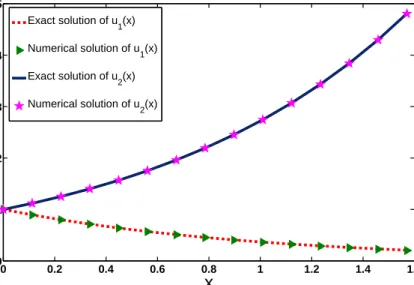
We now consider an example to illustrate how to solve an initial-value heat problem in the infinite domain. More specifically, we consider the following system:
∂u ∂τ(x, τ) = 4 ∂2u ∂x2(x, τ),−∞< x <+∞, τ >0, u(x,0) =ex, u(x, τ)∼ex asx→ ±∞, (2.2.19)
which has a unique solution u(x, τ) =ex+4τ.
Using the formula (2.2.18) with a= 2 and f(x) =ex, we easily obtain the solution of the system (2.2.19) as follows: u(x, τ) = 1 4√πτ Z +∞ −∞ eξe−(x16−ξτ)2dξ= 1 4√πτ Z +∞ −∞ e−(x−ξ16+8ττ)2+4τ+xdξ.
Using the variable transformation: z= x−ξ+ 8τ
4√τ , the solution of the system (2.2.19) can be
expressed as: u(x, τ) = √1 π Z +∞ −∞ e−z2ex+4τdz =ex+4τ.
Therefore, we obtain the unique solution of the system.
We are now ready to solve the system (2.2.16) to obtain the closed-form Black-Scholes formula for European vanilla options.
2.2.4 The Black-Scholes formula
Using the formula (2.2.18) with a= 1 and f(x) = max(e(1−α)x−e−αx,0), we easily obtain the solution of the system (2.2.16) as follows:
C(x, τ) = Z +∞ −∞ max(e(1−α)ξ−e−αξ,0)e− (x−ξ)2 4τ 2√πτ dξ= Z +∞ 0 (e(1−α)ξ−e−αξ)e− (x−ξ)2 4τ 2√πτ dξ = 1 2√πτ Z +∞ 0 e−(x−ξ+2(14τ−α)τ)2+(1−α)2τ+(1−α)xdξ | {z } I −2√1 πτ Z +∞ 0 e−(x−ξ−4τ2ατ)2+α2τ−αxdξ | {z } J .
Using the variable transformations: u = x−ξ+ 2(1√ −α)τ
2τ and v =
x−ξ−2ατ
√
2τ to the
integrals I and J, respectively, C(x, τ) can be expressed as:
C(x, τ) = e(1−α)2τ+(1−α)x√1 2π Z x+2(1−α)τ √ 2τ −∞ e−u22du−eα2τ−αx√1 2π Z x−2ατ √ 2τ −∞ e−v22dv = e(1−α)2τ+(1−α)x N(x+ 2(1√ −α)τ 2τ )−e α2τ−αx N(x−√2ατ 2τ ), where N(x) = √1 2π Z x −∞
e−u2/2du, the cumulative distribution function of the standard nor-mal distribution.
Converting the solution to the original coordinate space (S, t), with the notice that
α2+β=−γ, (1−α)2+β =−q, we obtain: V(S, t) = Eeαx+βτC(x, τ) =M1(S, T −t, E), where M1(x, y, z) =xe−δyN(d1(x, y, z))−Ee−ryN(d2(x, y, z)), d1(x, y, z) = ln(x/z) + (r−δ+σ2/2)y σ√y , d2(x, y, z) =d1(x, y, z)−σ √y. (2.2.20)
2.3 The integral representation of American vanilla options
The integral representation of the price of an American vanilla option has been studied in a number of works [20, 49, 52, 54]. Particularly, readers are referred to [20] for a detailed review on this. In this section, we will recall the derivation of this integral representation by using the (incomplete) Fourier transform technique. The purpose of doing this is to familiarize readers with the solution procedure and necessary techniques that can be extended for pricing more complicated American-style options.
Under the Black-Scholes framework, the price of an American vanilla call depends on the underlying asset priceS, the current timetand other constant parameters: the exercise price
E, the volatility rate σ, the risk-free interest rate r, the dividend rate δ and the expiry time
T. Let V(S, t) be the option price associated with the underlying asset price S and time t. Typically, at each time t during the life of the option, there exists an unknown value of the underlying asset referred to as the optimal exercise price denoted by Sf(t), above which the option should be exercised immediately and its value is then equal to the payoff received by exercising the option. As a result, we only need to price the option when the asset price is below this optimal exercise boundary. The pricing domain I of the option can be expressed mathematically as:
I ={(S, τ)|0≤S ≤Sf(τ),0≤t≤T}.
Using arguments similar to those used in Section 2.2.2, it can be shown that V(S, t) satisfies equations (2.2.10)-(2.2.12). In addition, in order to determine the optimal exercise boundary, the following smooth pasting conditions are needed [12]:
V(Sf(t), t) =Sf(t)−E,
∂V
∂S(Sf(t), t) = 1. (2.3.21)
any tis given by: A ∂V ∂t + σ2S2 2 ∂2V ∂S2 + (r−δ)S ∂V ∂S −rV = 0, V(S, T) = max(S−E,0), V(Sf(t), t) =Sf(t)−E, ∂V ∂S(Sf(t), t) = 1, lim S→0V(S, t) = 0, (2.3.22) whereA is defined ont∈[0, T], S ∈[0,∞).
To make the system A even simpler, we use the same dimensionless variables defined in (2.2.15), with an extra one: xf(τ) = ln
Sf(t)
E . Under this variable transformation, the
system (2.3.22) now becomes a dimensionless system, which includes a standard heat equation together with the corresponding initial and boundary conditions:
B ∂C ∂τ(x, τ) = ∂2C ∂x2(x, τ), C(x,0) =f(x), C(xf(τ), τ) =g1(xf(τ), τ), ∂C ∂x(xf(τ), τ) =g2(xf(τ), τ), lim x→−∞C(x, τ) = 0, (2.3.23)
wheref, g1, g2 are functions defined as:
f(x) = max(e(1−α)x−e−αx,0),
g1(x, y) =e(1−α)x−βy−e−αx−βy,
g2(x, y) = (1−α)e(1−α)x−βy+αe−αx−βy. (2.3.24)
As shown in [20], this system can be efficiently solved by using the Fourier transform. The Fourier transform of an arbitrarily continuous function f(x), denoted by F{f(x)}, is defined
as:
Ff(x) ≡U(ω) =
Z ∞
0
f(x)eiωxdx,
with the corresponding inversion:
f(x)≡ F−1U(ω) = 2
π
Z ∞
0
U(ω)e−iωxdω.
Here ω is called the Fourier transform parameter. It should be noted that a continuous function f(x) is Fourier transformable if R−∞+∞|f(x)|dx < ∞. Readers are referred to [66] to obtain some properties and applications of the Fourier transform in solving partial differential equations.
To apply the Fourier transform to the system (2.3.23), its x-domain first needs to be extended to an infinite domain first by expressing the PDE as:
H(xf(τ)−x)
∂C
∂τ (x, τ) =H(xf(τ)−x) ∂2C
∂x2(x, τ) (2.3.25)
whereH(x) is the Heaviside function, defined as:
H(x) = 1, if x >0, 1/2, if x= 0, 0, if x <0. (2.3.26)
The reason for the appearance of the factor of 1/2 at the point of discontinuity is explained in [20]. The initial and boundary conditions remain unchanged.
For the purposes of the transform method, we assume that the functionC(x, τ) and its first derivatives with respect toxcan be treated as zero whenxtends to infinity. This assumption is subsequently justified by virtue of the facts that the solution obtained after applying the Fourier transform satisfies the system (2.3.23), and that the solution of the system (2.3.23) is unique.
x. By definition, we have: F H xf(τ)−xC(x, τ) = Z xf(τ) −∞ C(x, τ)eiωxdx≡Cb(ω, τ),
where for convenience, Cb(ω, τ) denotes the Fourier transform of H xf(τ)−xC(x, τ). Direct calculation shows that:
F H xf(τ)−x ∂C ∂τ(x, τ) = ∂Cb ∂τ(ω, τ)−x′f(τ)g1 xf(τ), τ eiωxf(τ), (2.3.27) and F H xf(τ)−x ∂2C ∂x2(x, τ)
=g2 xf(τ), τeiωxf(τ)−iωeiωxf(τ)g1 xf(τ), τ−ω2Cb(ω, l). (2.3.28) Note that here the notation x′
f(τ) denotes the first derivative of xf with respect to τ, and
g1, g2 are predetermined functions defined in (2.3.24).
As a result of applying the Fourier transform with respect to x, the PDE (2.3.25) can be reduced to the following linear first-order ODE in the Fourier space:
∂Cb
∂τ(ω, τ) +ω
2Cb(ω, τ) =G(ω, τ)
where
G(ω, τ) =eiωxf(τ)g
2 xf(τ), τ−iωeiωxf(τ)g1 xf(τ), τ+x′f(τ)g1 xf(τ), τeiωxf(τ) with initial condition Cb(ω,0) =
Z xf(τ)
−∞
f(x)eiωxdx.
The solution of this initial-value ODE can be easily solved as:
b
C(ω, τ) =Cb(ω,0)e−ω2τ +
Z τ
0
e−ω2(τ−ξ)G(ω, ξ)dξ. (2.3.29) As Cb(ω, τ) denotes the Fourier transform of H xf(τ)−xC(x, τ), from (2.3.29), we can
now express the solution of the system (2.3.23) as follows: H xf(τ)−xC(x, τ) =F−1 b C(ω,0)e−ω2τ +F−1 Z τ 0 e−ω2(τ−ξ)G(ω, ξ)dξ . (2.3.30) Furthermore, as S =Eex, Sf(τ) = Eexf(τ), and V(S, t) =Eeαx+βτC(x, τ), by multiplying
Eeαx+βτ to both sides of (2.3.30), we can express the solution of the system (2.3.22) as follows:
H lnSf(t)−lnSV(S, t) = Eeαx+βτF−1 b C(ω,0)e−ω2τ (2.3.31) +Eeαx+βτF−1 Z τ 0 e−ω2(τ−ξ) G(ω, ξ)dξ .
The first and second terms in the right hand side of (2.3.31) clearly need to be calculated explicitly in order to obtain an integral representation for the solution of the system (2.3.22).
Compute the first term of (2.3.31).
We first calculate the inverse Fourier transform of e−ω2τ
as: F−1{e−ω2τ}= 2 π Z +∞ −∞ e−ω2τe−iωxdω= e− x2 4τ 2√πτ.
Applying the Convolution theorem for the Fourier transform [66], we obtain:
F−1{Cb(ω,0)e−ω2τ }=F−1 ( FnH(xf(0)−x)f(x) o Fne− x2 4τ 2√πτ o) = Z +∞ −∞ H(xf(0)−u)f(u) e−(x−4τu)2 2√πτ du= Z xf(0) −∞ maxe(1−α)u−e−αu,0e− (x−u)2 4τ 2√πτ du = 1 2√πτ Z xf(0) 0 e(1−α)u−(x−4τu)2du− 1 2√πτ Z xf(0) 0 e−αu−(x−4τu)2du = e (1−α)2τ+(1−α)x 2√πτ Z xf(0) 0 e−(x−u+2(14τ−α)τ)2du−e α2τ−αx 2√πτ Z xf(0) 0 e−(x−u−4τ2ατ)2du.
By using the variable transformations v = x−u+ 2(1√ −α)τ
2τ and w =
x−u−2ατ
√
last two integrals, respectively, we obtain: F−1{Cb(ω,0)e−ω2τ} = e (1−α)2τ+(1−α)x √ 2π Z x+2(1−α)τ √ 2τ x−xf(0)+2(1−α)τ √2 τ e−v 2 2 dv −e α2τ−αx √ 2π Z x−2ατ √2 τ x−xf(0)−2ατ √ 2τ e−w22dw = e(1−α)2τ+(1−α)x N x+ 2(1−α)τ √ 2τ −N x−xf(0) + 2(1−α)τ √ 2τ −eα2τ−αx N x−2ατ √ 2τ −N x−xf(0)−2ατ √ 2τ (2.3.32)
Consequently, the first term of (2.3.31) can be expressed as:
Eeαx+βτF−1
b
C(ω,0)e−ω2τ
=M1(S, T −t, E)−M1(S, T −t, Sf(T)), (2.3.33) whereM1 is a function of three variables defined in (2.2.20).
Compute the second term of (2.3.31).
F−1 Z τ 0 e−ω2(τ−ξ)G(ω, ξ)dξ = Z τ 0 F −1e−ω2(τ−ξ) G(ω, ξ)dξ = 1 2π Z τ 0 Z +∞ −∞ e−ω2(τ−ξ)−iω(x−xf(ξ))g 2(xf(ξ), ξ) +x′f(ξ)g1(xf(ξ), ξ)−iωg1(xf(ξ), ξ)dωdξ = 1 2π Z τ 0 g2(xf(ξ), ξ) +x′f(ξ)g1(xf(ξ), ξ) Z +∞ −∞ e−ω2(τ−ξ)−iω(x−xf(ξ))dωdξ −21π Z τ 0 ig1(xf(ξ), ξ) Z +∞ −∞ ωe−ω2(τ−ξ)−iω(x−xf(ξ))dωdξ = Z τ 0 g2(xf(ξ), ξ) +x′f(ξ)g1(xf(ξ), ξ) e− (x−xf(ξ))2 4(τ−ξ) 2pπ(τ−ξ)dξ − Z τ 0 g1(xf(ξ), ξ) x−xf(ξ) 4pπ(τ−ξ)3e −(x−4(xfτ−(ξξ)))2dξ = Z τ 0 e− (x−xf(ξ))2 4(τ−ξ) 2pπ(τ −ξ) g2(xf(ξ), ξ) +g1(xf(ξ), ξ) x′ f(ξ)− x−xf(ξ) 2(τ−ξ) dξ = J(x, τ),
whereJ is a function of two variables and is defined as: J(x, y) = Z τ 0 e− (x−xf(ξ))2 4(y−ξ) 2pπ(y−ξ) g2(xf(ξ), ξ) +g1(xf(ξ), ξ) x′ f(ξ)− x−xf(ξ) 2(y−ξ) dξ. (2.3.34) Hereg1, g2 are defined in (2.3.24). By substitutingg1 andg2 in the formula ofJ(x, τ), we can
express: J(x, τ) =J1(x, τ; 1−α)−J1(x, τ;−α), where J1(x, τ; 1−α) = Z τ 0 e− (x−xf(ξ))2 4(τ−ξ) +(1−α)xf(ξ)−βξ 1 2pπ(τ−ξ) 1−α+x′f(ξ)−x−xf(ξ) 2(τ−ξ) dξ =− Z τ 0 ∂ ∂ξ x−xf(ξ) + 2(1−α)(τ −ξ) p 2(τ −ξ) ! e− (x−xf(ξ)+2(1−α)(τ−ξ))2 4(τ−ξ) +(1−α)2(τ−ξ)−βξ+(1−α)xdξ =−e(1−α)x+(1−α)2τ Z τ 0 e−((1−α)2+β)ξ ∂ ∂ξN x−xf(ξ) + 2(1−α)(τ −ξ) p 2(τ−ξ) ! dξ =−e(1−α)x+(1−α)2τ lim ξ→τe −((1−α)2+β)ξ N x−xf(ξ) + 2(1p −α)(τ −ξ) 2(τ −ξ) ! +e(1−α)x+(1−α)2τ N x−xf(0) + 2(1−α)τ √ 2τ −e(1−α)x+(1−α)2τZ τ 0 ((1−α)2+β)e−((1−α)2+β)ξ N x−xf(ξ) + 2(1p −α)(τ −ξ) 2(τ −ξ) ! dξ.
We can also obtain J1(x, τ;−α) by simply replacing 1−α by α in the above formula of
J1(x, τ; 1−α). Therefore, J(x, τ) = −e(1−α)x+(1−α)2τ eqτ1x=xf(τ)−N x −xf(0) + 2(1−α)τ √ 2τ +e(1−α)x+(1−α)2τ Z τ 0 qeqξN x−xf(ξ) + 2(1p −α)(τ −ξ) 2(τ −ξ) ! dξ +e−αx+α2τ eγτ1x=xf(τ)−N x−xf(0)−2ατ √ 2τ −e−αx+α2τZ τ 0 γeγξN x−xfp(ξ)−2α(τ −ξ) 2(τ −ξ) ! dξ,
where 1x=xf(τ)(x) = 1 2 if x=xf(τ), 0 if x6=xf(τ). The second term of (2.3.31) can be now calculated explicitly as
Eeαx+βτF−1 Z τ 0 e−ω2(τ−ξ) G(ω, ξ)dξ = −(S−E)1S=Sf(t)+M1(S, T −t, Sf(T)) + Z T t Q1(S, t, u, Sf(u))du, (2.3.35) where 1S=Sf(t)(S) = 1 2 if S =Sf(t), 0 if S6=Sf(t), (2.3.36)
and Q1 is a function of four variables defined by:
Q1(x, y, z, w) =xδe−δ(z−y)N(d1(x, z−y, w))−Ee−r(z−y)N(d2(x, z−y, w)). (2.3.37)
Here M1, d1, d2 are functions already defined in (2.2.20).
Using results in (2.3.33) and (2.3.35), the solution of the system (2.3.22) can be expressed as: H lnSf(t)−lnSV(S, t) =−(S−E)1S=Sf(t)+M1(S, T−t, E) + Z T t Q1(S, t, u, Sf(u))du. (2.3.38) The expression (2.3.38) is the integral representation of the price of an American vanilla call. This integral representation expresses the value of an American vanilla call as the sum of the value of its European counterpart and the early exercise premium, which depends on the optimal exercise functionSf(t). To calculate the price of the American vanilla call, we need to determine Sf(t), which is governed by the following integral equation (derived by letting
S =Sf(t) in (2.3.38)):
Sf(t)−E =M1(Sf(t), T −t, E) +
Z T
t
Q1(Sf(t), t, u, Sf(u))du, (2.3.39) where functions M1 and Q1 are defined in (2.2.20) and (2.3.37), respectively.
The pricing problem of American vanilla calls is now reduced to solving an integral equa-tion. In the next section, we will recall some concepts, techniques to solve integral equations.
2.4 Integral equations
In general, an integral equation is an equation in which the unknown function appears inside the integral sign. A typical form of an integral equation, with the unknown u(x), is of the form:
u(x) =f(x) +λ
Z β(x)
α(x)
K(x, t, u(t))dt, (2.4.40) whereK, α, β, f are given functions andλis a constant parameter. Hereα, β are called limits of the integration.
The most frequently used integral equations fall under two major classes, namely Fredholm and Volterra integral equations. They are classified based on whether the limits of integration are fixed constants or at least one limit is a variable. More precisely, a typical Fredholm integral equation is of the form:
u(x) =f(x) +λ
Z b
a
K(x, t, u(t))dt.
On the other hand, a typical Volterra integral equation is of the form:
u(x) =f(x) +λ
Z x
a
K(x, t, u(t))dt,
wherea, b are constant.
Integral equations can also be categorized as linear or nonlinear integral equations, which depend on whether the functionKin (2.4.40) is linear or not with respect to the unknownu(x), respectively. Many linear integral equations and some simple nonlinear integral equations can be solved analytically by using powerful techniques such as Adomian decomposition method

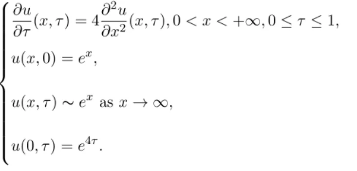
![Table 3.1 presents a comparison of the prices of the American-style down-and-out calls without rebate calculated by using the IE method with those reported in [85]](https://thumb-us.123doks.com/thumbv2/123dok_us/10974955.2985505/77.918.199.811.443.682/table-presents-comparison-prices-american-rebate-calculated-reported.webp)