https://doi.org/10.1007/s10846-018-0809-5
A Real-Time 3D Path Planning Solution for Collision-Free Navigation
of Multirotor Aerial Robots in Dynamic Environments
Jose Luis Sanchez-Lopez1,2,4 ·Min Wang1·Miguel A. Olivares-Mendez1·Martin Molina3,4·Holger Voos1
Received: 17 October 2017 / Accepted: 1 March 2018
©Springer Science+Business Media B.V., part of Springer Nature 2018 Abstract
Deliberative capabilities are essential for intelligent aerial robotic applications in modern life such as package delivery and surveillance. This paper presents a real-time 3D path planning solution for multirotor aerial robots to obtain a feasible, optimal and collision-free path in complex dynamic environments. High-level geometric primitives are employed to compactly represent the situation, which includes self-situation of the robot and situation of the obstacles in the environment. A probabilistic graph is utilized to sample the admissible space without taking into account the existing obstacles. Whenever a planning query is received, the generated probabilistic graph is then explored by an A discrete search algorithm with an artificial field map as cost function in order to obtain a raw optimal collision-free path, which is subsequently shortened. Realistic simulations in V-REP simulator have been created to validate the proposed path planning solution, integrating it into a fully autonomous multirotor aerial robotic system.
Keywords Path planning·Obstacle avoidance·Dynamic environments·Aerial robotics·Multirotor·UAV·MAV· Remotely operated vehicles·Mobile robots
1 Introduction
In order to enable new robotic applications in modern life such as package delivery, search and rescue, or surveillance, it is essential for future small multi-rotor aerial robots, also known as drones or unmanned aerial systems (UAS), to incorporate deliberative capabilities. They allow the robot
Jose Luis Sanchez-Lopez [email protected] Holger Voos
1 Automation and Robotics Research Group (ARG), Interdisciplinary
Center for Security, Reliability and Trust (SnT), University of Luxembourg, 29, avenue J. F. Kenedy, 1855 Luxembourg, Luxembourg
2 Center for Automation and Robotics (CAR), CSIC-UPM,
Calle Jose Gutierrez Abascal 2, 28024 Madrid, Spain
3 Department of Artificial Intelligence, Technical University
of Madrid (UPM), Campus de Montegancedo S/N 28660 Boadilla del Monte, Madrid, Spain
4 Computer Vision and Aerial Robotics (CVAR), Technical
University of Madrid (UPM), Madrid, Spain
www.vision4uav.eu
to look ahead in time and generate a task to be performed taking into account the current states of both the robot and environment, and predicting the potential consequences of the planned behaviors in the future. Trajectory planning, as a crucial deliberative capability, is the ability to generate a feasible collision-free set of motion commands which can be executed by the robot, in order to reach a particular desired state, called the goal.
A useful trajectory planner needs to be able to generate feasible collision-free trajectories fast enough so as to enable efficient reactions to changes in the goal, in the environment, or in the state of the robot. This is especially critical in aerial robots, since their unstable nature does not allow them to passively wait for a slow response from the trajectory planner.
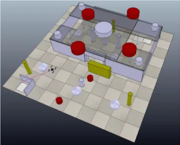
Additionally, complex and highly dynamic environment (such as the ones represented in Figs.12and21) poses great challenges for both collision-free planning components and perception components, as such environment is constantly changing and consists of both moving and static objects. The perception components are responsible for estimating the state of the environment using a representation that is useful for the planning components. Therefore, they are highly related.
Before continuing, it is important to clarify the difference between the concepts of path and trajectory. According to Aguiar and Hespanha [2], a path is a continuous function that connects two points of any particular space. A trajectory is defined as a path with explicit parametrization of time and therefore, specifications on velocity, acceleration, jerk, etc. are introduced.
Commonly used multirotor aerial robots are under-actuated, i.e. they only have four controllable inputs to move in a higher dimensional space. This type of aerial robots are non-holonomic systems in their complete state space (i.e. pose, velocity, and acceleration), i.e. its state depends on the trajectory taken in order to achieve it. Moreover, planning collision-free trajectories requires knowledge of not only constraints and state of the aerial robot but also constraints and state of the environment where the robot performs, which increases the complexity of search for a feasible collision-free trajectory.
For simplifying the complexity of the feasible collision-free trajectory search problem, a slow-motion (near-hovering) assumption can be used. This assumption is valid for trajectory planning as long as aggressive maneuvers such as flips are not required, it is therefore eligible for aforementioned appli-cations. With this assumption the state of aerial robots can be simplified to their heading (yaw angle) and their position, which makes them holonomic systems.
The trajectory planning problem can be executed sequen-tially, as proposed in Richter et al. [29], with first of all a collision-free path planning and afterwards the post-processing of this path to obtain a feasible collision-free trajectory.
A typical solution adopted for complex and highly dynamic environment is to incorporate two layers in the path planning system, ros [1], one capable of finding a global solution for the complex problem without considering the dynamic objects of the environment, and the other able to obtain a local solution (which can be deliberative or reactive) for the collision avoidance of dynamic obstacles that are in the vicinity of the robot. Despite having demonstrated their performance in multiple applications, these two layered path planning systems are not capable of finding an optimal solution for the complete problem of navigating in a complex dynamic environment.
This paper, as the continuation of our previous work, Sanchez-Lopez et al. [37], presents a single layered 3D deliberative path planning solution for the collision-free navi-gation of multirotor aerial robots in dynamic environments. Our path planner incorporates a single layer to obtain an optimal feasible collision-free path in a complex dynamic environment formed by static and moving objects. The situation, including the self-situation (the situation of the aerial robot itself) and the situation of the environment, is compactly represented by high-level geometric primitives. More-over, to reduce the computational cost of the planner, the
admissible space is sampled at launching time, i.e. with-out incorporating information of the objects present in the environment, by means of a probabilistic graph. At query time, the probabilistic graph is explored by a discrete search algorithm, i.e. A algorithm, to find an optimal raw collision-free path. To guarantee the generated path is collision-free and also speed up the search, an artificial potential field map is employed by the discrete search algo-rithm as its cost function. Finally, the obtained raw path is shortened.
Despite being a single-layered approach, the proposed collision-free path planner is able to operate real-time and tackle complex dynamic environments, as the following features are in place: (1) compact definition of the situation; (2) sampling of the admissible space at launching time without the need of modifying it when the situation changes; (3) utilization of an artificial potential field map as a cost function of the discrete search algorithm, which incorporates the situation of the obstacles in the environment; (4) usage of a search algorithm, which guarantees optimality of the collision-free path, if exists. To the best of our knowledge, this is the first 3D collision-free path planner for multirotor aerial robots, real-time capable, and specially designed for highly dynamic environments.
The contributions of this paper, when compared to our previous work, [37], are as follows: (1) extension from 2D to 3D spaces; (2) adaptation of the representation of the work-space for 3D environments; (3) enhanced definition of the admissible space, incorporating concepts imported from control theory, (4) refined description of the artificial potential field map, which improves the quality of the collision-free path; (5) improved design of the path planning solution with newly added functionalities.
The remainder of the paper is organized as follows: Section 2 presents an overview of the state of the art on path planning. Section 3introduces the complete solution of the proposed path planning, which is composed of two parts, as described below. The core functionality of the presented solution, i.e. the path planning, is detailed in Section 4, whereas newly added functionalities are presented in Section 5. In Section 6, the proposed path planning solution is validated through simulations and real experiments. Finally, Section 7 concludes the paper and points out some future work lines. We recommend the reader to print the paper in color, as the images it contains are complex and color is needed to follow them.
2 Related Work
Path planning for robotic applications as a research topic has been actively studied in recent years. While most works focus only on 2-dimensional (2D) or 2.5-dimensional
(2.5D) methods, approaches for 3D path planning remain less explored. Nevertheless, different types of approaches such as node-based optimal algorithms, sampling based algorithms, and bioinspired algorithms have been proposed for tackling 3D path planning in the literature, Yang et al. [44].
Node-based optimal algorithms, also called discrete search algorithms, aim to search for an optimal collision-free path through a generated node network (or grid map). For 3D environment path planning, A algorithm, Hart et al. [8] and Dechter and Pearl [7], has been a popular choice among others due to its fast search ability. However it is only limited to tackling static environments. The counterpart D, Stentz [39], on the other hand, is able to deal with dynamic environments, though can produce unrealistic distance.
Another widely implemented family of algorithms is sampling-based algorithms, including rapidly-exploring random trees (RRT), LaValle [16], Probabilistic Road Maps (PRM), Kavraki et al. [13], visibility graph, Lacasa et al. [15], and Artificial Potential Field (APF), Hwang and Ahuja [11]. In general, this kind of algorithms requires mathematical representation for the workspace. They sample the environment in various forms such as a set of nodes or cells, and then either map the environment or search randomly in order to obtain a feasible path. Therefore, according to Yang et al. [44], APF is categorized, as a sampling-based algorithm.
In comparison to node-based optimal algorithms, mathe-matic model-based algorithms use kinodynamic constraints in conjunction with polynomial forms to optimize path plan-ning, while the former utilize grids to describe configuration space with the assumption that robot is a point and that only acceleration and velocity constraints are considered. Exam-ples of these types of algorithms are linear algorithms e.g. Mixed-Integer Linear Programming (MILP) methods, Yue et al. [46], and optimal control algorithms e.g. Tisdale et al. [41].
Bioinspired algorithms stem from imitating the behavior of humans or other natural creatures with the motivation to enable algorithms to learn by themselves from their own experience. In general, they do not rely on complex environment models to reach a near optimal solution. This type of algorithms is often used when general mathematic model-based algorithms fail or trapped into local minimum. However, algorithms of this type generally have high time complexity and their performance may vary significantly depending on the model diagrams. Popular examples of bioinspired algorithms are neural networks (NN), Kassim and Kumar [12], Particle Swam Optimization (PSO), Kennedy [14], genetic algorithm (GA), Holland [9], etc.
Each type of aforementioned algorithms has their advantages and disadvantages. In order to be able to cope with increasingly complex 3D environments in robotics
applications, recent research efforts have been made to overcome the shortcomings of individual algorithms by exploring different combinations among them and beyond.
In Liu et al. [18], a search based planning method incorporating discretized optimal control problem solving was proposed for fast online replanning during continuous flight. Lin and Saripalli [17] proposed a method based on the closed-loop RRT algorithm and developed three variations of it to handle different types of aerial robots and varying dynamic obstacle conditions. Arantes et al. [3] combined visibility graph with a multi-population genetic algorithm. Chen et al. [6] fused APF with optimal control theory. A multi-layered path planning approach is proposed in Nieuwenhuisen et al. [22], which employs a mission planning layer consisting of global and local path planning and a reactive layer based on APF. Hossain and Ferdous [10], developed a path planning method based on Bacterial Foraging Optimization (BFO) technique, Gaussian cost function and a high level decision strategy and results are compared with PSO method. Yao et al. [45] introduced a 3D path-planning algorithm based on interfered fluid flow for dynamic obstacle obstacle avoidance. Yan et al. [43] illustrated a 3D path planning approach which utilizes random sampling in a bounding box in the whole 3D space to improve the efficiency of PRM, and then applies A algorithm to the generated roadmap for feasible path generation. Narayanan et al. [21] presented an anytime planner which is essentially a fast Avariant based on time interval for dynamic path planning.
3 Path Planning Solution
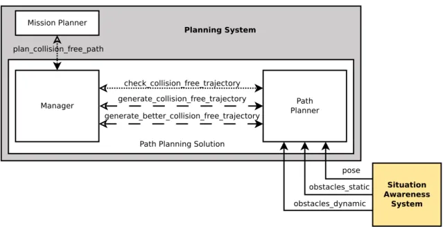
The complete path planning solution is formed by two components: the manager and the path planner. Both components use three different paradigms for inter and intra communication: data streams, request/reply tasks (called services), and preemptable tasks (called actions). This path planning solution is shown in Fig.1.
The main functionality of the planner component (as explained in Section 4) is the generation of collision-free paths given a goal and taking into account the estimated pose of the aerial robot in world coordinates, and the estimated information relative to the static and dynamic objects existing in the environment. The situational awareness information is provided by the situation awareness system in the required format and it is received through three different data streams. This collision-free path is calculated thanks to a provided service, whose request is the goal to achieve, and whose reply is that calculated collision-free path.
Besides, in a parallel execution thread, the path planner includes an action that, when enabled, it continuously
Fig. 1 Path planning solution. It is formed by two components: the manager and the path planner. The continuous lines represent the data streams; the dashed lines, the services; and the dotted lines, the actions.
In both services and actions, the black arrows represent the server side, whereas the white arrows encode the client side
checks if a given free path remains collision-free despite the changes in the situation awareness (see Section5.1).
Furthermore, once again in a parallel execution thread, the path planner provides a service that calculates a better collision-free path, if any, in terms of cost (as described in Section 5.2). The request of this service is the goal to achieve and the reference collision-free path. Its reply is the new collision-free path, if any.
The manager handles the path planner component, acting as an intermediary with the mission planner. It receives the goal to achieve given by the mission planner, by means of an action that it provides, continuously returning the most optimum collision-free path despite the changes in the situation (both self-localization and environment). It requests the path planner the generation of a collision-free path, activating the collision-collision-free check action after receiving it. Whenever the collision-free check is not passed, it requests again the path planner the generation of a free path. Moreover, in parallel to the free check, the manager cyclically calls the better collision-free generation service to find a new optimum collision-collision-free path.
4 Path Planning Algorithm
This section presents the proposed algorithm for the generation of collision-free paths, which is implemented as a service of the path planner component presented in Section3.
4.1 Work Space
The work space incorporates the knowledge of the complete situation, including the self-situation and the situation of the environment. This situation knowledge is given by the situation awareness system, but the presented planning algorithm imposes the kind of descriptor required.
The proposed path planning algorithm describes the situation by means of high-level geometric primitives (see Section4.1.1) unlike other commonly used more computationally expen-sive representations such as grid maps or octrees, [42]. The main advantages of this simplified environment representa-tion are (1) compact descriprepresenta-tion of the environment without loss of resolution (i.e. no need of approximations), and (2) capability of easily handle dynamic environments.
Moreover, the presented path planning algorithm distin-guishes between static and dynamic objects included in the environment (see Section4.1.2).
4.1.1 Situation Described with High-Level Geometric Primitives
All the objects of the environment including the aerial robot itself are described as a set of uniquely labeled high-level geometric primitives. As mentioned, using this environment representation reduces the required information to com-pletely describe it, but without the need of approximations (e.g. a cylinder has to be approximated when using an octree to describe the environment). This contributes to reduce the complexity of the distance to an object evaluation whenever is required, speeding up the planning algorithm.
For simplicity, our proposed approach only implements three kinds of high-level geometric primitives to describe objects of the environment: cuboids, cylinders, and ellip-soids. The parameters that describe the implemented high-level geometric primitives are:
– Pose (position and orientation) of the center of the reference frame attached to the object in world coordinates,pWO= {tWO,qWO}.
– Dimensions of the object, rO =
rx, ry, rz
T
. For ellipsoids, their radii are used; while for cuboids, the dimension of their sides are used; and for cylinders, the two first parameters describe their radii, and the third one their height.
It is important to highlight that the robot situation is as well described by means of high-level geometric primitives, once again, without the need of approximations. For simplicity, our proposed path planning algorithm assumes that the shape of the robot is a cylinder.
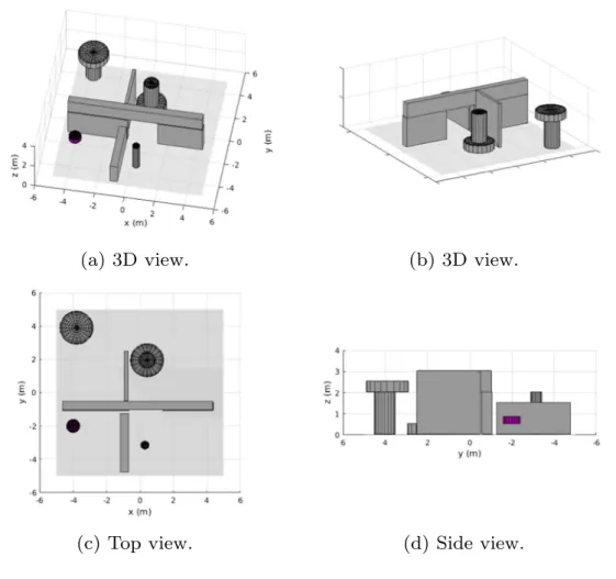
Figure2shows an example of a work space.
It is worth to mention that for the sake of completeness, our algorithm is not limited to the previously presented three kinds of high-level geometric primitives. In general, any kind of geometric primitive might be used for the
situation description (e.g. planes, pyramids, cones, barrels, etc). Moreover, an object of the environment with a complex shape might be described as a set of simple geometric primitives. Furthermore, if an object has a very complex shape that cannot be easily described as a set of geometric primitives, other kinds of representation can be used, such as an octree including exclusively the shape information of this object.
4.1.2 Distinction Between Static and Dynamic Objects of the Environment
As mentioned before, the presented path planning algorithm distinguishes between static and dynamic objects included in the environment. This distinction allows to ignore the moving objects whenever they are far enough from the robot (in the admissible space explained below), i.e. distance between them is greater than a configurable threshold which depends on the velocity of the moving objects. That implies the fact that the moving objects will most likely change their current pose before the robot reaches that point whenever they are far, which thus simplifies the path planning query.
It is worth to mention that our path planner do not take advantage of the dynamic part of the situation information
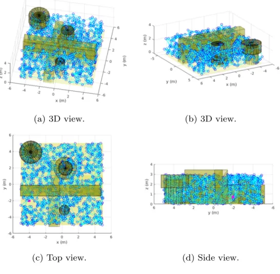
Fig. 2 Environment formed by several cuboids and cylinders (gray). The robot is represented by a purple cylinder whose center is at the point
tW
R =[−4,−2,0.7]T with an orientationqW
(i.e. velocity and acceleration) of the moving objects, remaining as a future work. Despite this, our path planner is capable of handling dynamic environments as it is able to plan collision-free paths in a reduced time thanks to its features listed in Section1and detailed along Section4. 4.2 Admissible Space
The work space (presented in Section4.1),W, is included in the Lie group SE(3) space, W ∈ SE(3), which has dimension 6. It has to be converted to a space, called admissible space,A, where the collision-free path can be searched taking into account all the restrictions of the robot.
4.2.1 Configuration Space
The configuration space,C, is a space that maps the work space into a space where the search of the collision-free path is possible and simplified. In the presented path planner, the state of the robot is simplified to its pose (i.e. velocity and acceleration is not considered). Also, as mentioned before in Section4.1.2, the dynamic part of the situation information (i.e. velocity and acceleration) of the
moving objects is not taken into account. Therefore, the configuration space is defined as a 6-dimensional space that is directly generated using the work space. Moreover, in the configuration space, the objects included in the work space, are dilated taking into account the dimensions of the robot using the Minkowski addition. It is important to highlight that the objects dilating is done along the 6 dimensions of the configuration space, i.e. it does not only depends on the position, but also depend on the orientation of the robot. For example, if the robot is described as a cylinder, the objects dilation clearly depends on the orientation of this cylinder.
To be able to plan a collision-free path, the previously defined configuration space cannot be used. It might be possible that some parts of the state of the situation cannot be perceived (e.g. the pitch and the roll of the aerial robot cannot be observed). It might be also possible that some parts of the state of the robot cannot be directly modified to reach the goal and are imposed (e.g. the planner cannot modify the yaw angle of the aerial robot and it is externally imposed). To overcome these limitations of the configuration space, we need to incorporate in a new space all the imposed restrictions on the motion, together with the restrictions on the perception of the situation. In this new
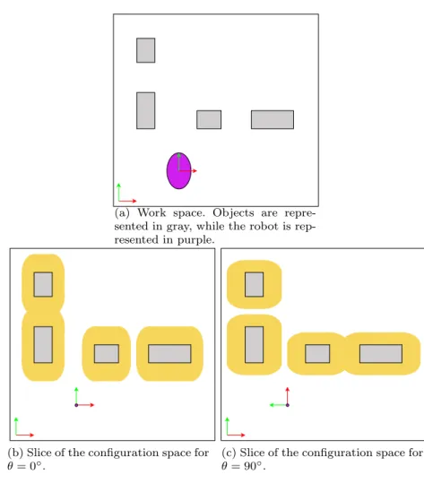
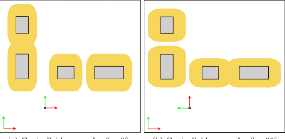
Fig. 3 Simple example to illustrate the concepts introduced in this section
Fig. 4 Observable space of the example introduced in Fig.3in the case thatθis not observable
space, the search of the collision-free path can be done. To define this space, we use two intermediate spaces that are inspired by the state-space control theory: the observable space and the controllable space.
To illustrate the concepts introduced in this section, the simple example represented in Fig. 3 is used. In this example, an holonomic 2D elliptical robot with three degrees of freedom,x,y, andθcan move in the work space shown in Fig.3a. Its configuration space is 3-dimensional, and for illustration purposes, only two slices of it, for the limit values ofθ = 0◦ andθ = 90◦, are shown in Fig.3b and c, respectively.
4.2.2 Observable Space
First of all, we define the observable space,O, as a subspace of the configuration space,O⊆C that incorporates all the restrictions on the perception of the situation. For all the restrictions,i, on the perception of the situation, an infinite set ofjsubspaces of the configuration space,Ci,j for all the
jvalues that the restrictionican have. The observable space incorporate the worse case by means of:
O= ⊕∀i,jCi,j (1)
where⊕is the operation composition of subspaces. For example, in case that the pitch,φ, and roll,θ, of the aerial robot, are not observable, we have infinite restricted configuration spaces,Cφ,j andCθ,k, for all thej-values and k-values that the pitch and roll can have (φ, θ ∈ [−π, π]]), being the observable space, O, the worse case subspace defined as:
O=⊕∀j∈[−π,π]Cφ,j
⊕⊕∀k∈[−π,π]Cθ,k
In the presented path planner, the pitch and the roll components of the orientation the robot are not assumed to be available, and therefore, the observable space is a 4-dimensional subspace of the configuration space.
Following the example introduced in Fig.3, in the case thatθis not observable, while the other degrees of freedom are observable, the observable space is 2-dimensional, and it is shown in Fig.4.
4.2.3 Controllable space
Second, we define the controllable space,U, as a subspace of the configuration space,U ⊆ C that takes into account the non-modeled imposed restrictions on the motion. For every non-modeled imposed restrictions,i, on the motion, a subspace of the configuration space, Ci,αi for a value αi that the imposed restriction i takes, is generated. The
controllable space is the part of the configuration space that considers only all the imposed restrictions as:
U = ∩∀iCi,αi (2)
This controllable space changes constantly whenever the values of the imposed restrictions,αichange.
Fig. 5 Controllable space of the example introduced in Fig.3in the case thatθis not controllable
For example, in case that the yaw of the aerial robot,ψ, is externally imposed with a valueαψ, the controllable space
is defined as:
U =Cψ,αψ
In the presented path planner, only the position is assumed to be controllable, being the values of its orientation imposed but not modeled, and therefore, the controllable space is 3-dimensional. Note that for an aerial robot, the pitch and the roll are directly related to thexandy by means of its motion model. Nevertheless, for simplicity we assume that this relationship cannot be modeled, and therefore, we treat the pitch and the roll as a non-modeled imposed given values.
Continuing with the example introduced before, in Fig.3, if now, θ, instead of being not observable as before, is not controllable, while the other degrees of freedom are controllable, the controllable space is 2-dimensional. The controllable space depends on the values of the non-modeled imposed restriction, in this case, the value of θ. Figure 5 shows the controllable space for two different example values ofθ.
4.2.4 Valid Space
Once the observable and the controllable spaces are determined, the valid space,V, has to be defined, combining them as: V = ∩∀k ⊕∀i,jCi,j k,αk = ∩∀kOk,αk =U(O) (3)
that is, the controllable space considering the observable space instead of the configuration space.
In the presented path planner, the valid space is 3-dimensional.
4.2.5 Admissible Space
Finally, the valid space is mapped to the admissible space,
A, to find the control inputs needed to obtain a collision-free path to reach a goal.
In the proposed path planner, the control inputs are the position of the aerial robot, and it is assumed to be holonomic. Therefore, the mapping from the valid space to the admissible space is a unit transformation, and consequently, the admissible space is the same than the valid space.
Fig. 6 Admissible space of the example presented in Fig.2. The robot is located in the point
Figure 6 shows the admissible space of the example presented in Fig.2.
4.3 Probabilistic Graph
To reduce the time that the planner requires to find a collision-free path, the admissible space is probabilistically sampled. This probabilistic sampling generates n random points (also called nodes or vertices) following a uniform distribution within the admissible space boundaries. Then sampled points are connected by means of edges to their nearest m neighbors (called m-neighborhood), creating a probabilistic graph. The connection between any of two nodes of the probabilistic graph has to fall completely inside the admissible space. The generation of this probabilistic graph is the most computationally expensive operation.
The probabilistic graph is generated at launching time, and therefore, no knowledge of the objects existing on the work space is taken into account (as shown in Fig.7, continuing with the previous example). Whenever a static object is included in the situation awareness of the environment (i.e. a static object is mapped), the probabilistic
graph could be modified to remove its nodes that fall inside the objects.
The previously known knowledge of the static objects of the environment can be as well incorporated to the probabilistic graph by modifying the uniform sampling function of the node generation into a custom probability density function. Moreover, this custom probability density function might be adapted to include the a priori knowledge of existing important areas (e.g. corridors).
The number of nodesnof the probabilistic graph must be representative of the environment. If the robot is operating in an environment that is not very cluttered, the number of nodesnmight be reduced to decrease the complexity of the graph search and therefore the path planning time.
Whenever the path planner receives a planning query from the current state, x0, to the desired state, xf, their
values are converted to the admissible space, P0 and Pf
respectively, and connected to the probabilistic graph as temporary nodes, that are deleted from the graph once the search has finished.
This proposed probabilistic graph approach differs from other existing probabilist approaches such as PRM,
Fig. 7 Probabilistic graph with 1000 nodes and 6-neighborhood of the example presented in Fig.2. The robot is located in the pointP0=[−4,−2,0.7]T. The goal point isPf =[−3,1,1]T
Kavraki et al. [13], where the probabilistic graph is generated including the information of all the objects of the environment. On the one hand, our approach requires higher time to complete the search of a collision-free path as the graph includes some nodes that fall inside the obstacles. Nevertheless, on the other hand, it allows handling dynamic environments without the need of modifying the probabilistic graph (which is very computationally expensive).
4.4 Cost Function: Potential Field Map
To guide the collision-free search task, and to incorporate the knowledge of the objects of the environment, a potential
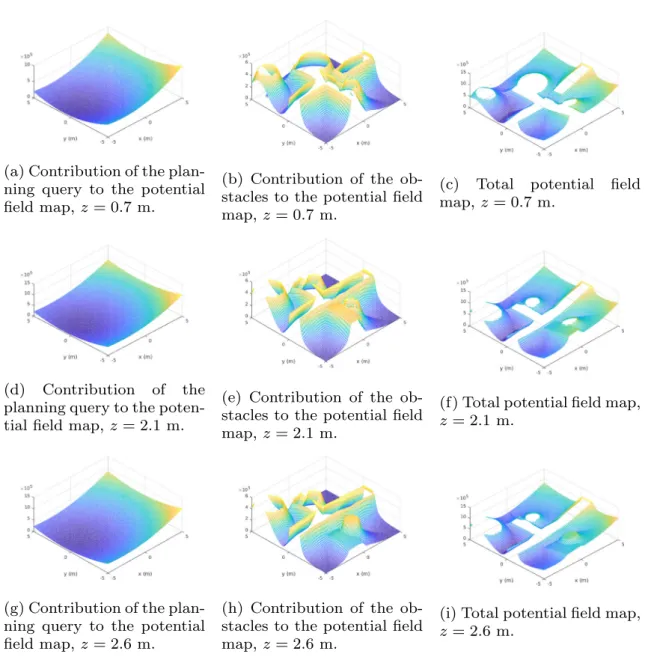
field map on the admissible space, that depends on the initial and desired state, is created as follows:
p(P )=pq(P )+pO(P ) (4)
where P is any point of the admissible space, pq is the
contribution to the potential field map of the planning query (see Section4.4.1), andpO is the contribution to the
potential field map of the obstacles of the environment (see Section4.4.2).
Figure8illustrates the concept of the potential field map following the previous example.
This concept of the potential field map has been previously introduced in Hwang and Ahuja [11], but used in a different way than presented in our work. In our work, the potential
Fig. 8 Different slices of the potential field map for a query fromP0 =[−4,−2,0.7]T toPf = [−3,1,1]T. For visualization purposes, the potential field map has be extracted for three different values ofz
field map is used to guide the graph search algorithm described in Section4.5 and therefore, our planner never falls in a local minima when calculating the collision-free path, computing always the most optimum path.
4.4.1 Potential Field Map of the Planning Query
To guide the search in the direction from the initial point,P0, to the target point,Pf, a potential field map cost function,
pq, is created.
The potential field map of the planning query,pq=pq
P , P0, Pf
, in a pointP of the admissible space given by its coordinatesxiP, is defined as an elliptic hyperparaboloid expression where the minimum is located inPf:
pq= ∀i xiP −xiPf 2 ci + d (5) being ci = ⎧ ⎪ ⎨ ⎪ ⎩ ∀i xP0 i −x Pf i 2 kr1i k0−kf , ifi=1 kr1i·c1, otherwise (6) d = kf (7)
where the coefficient kr1i determines the priority of the
planned movement in a specific directioni, when compared with the priority in the first direction; the coefficient k0 determines the value of the potential field map in the initial point; and the coefficient kf determines the value of the
potential field map in the final point. All these coefficients determine the aggressiveness in the search of the planner.
4.4.2 Potential Field Map of the Obstacles
To include the situation of the objects of the environment, being able to find a collision-free path in the probabilistic graph, a potential field map cost function,pO, is created.
The potential field map of the obstacles, O, of the environment, pO = pO(P , O), in a point P of the
admissible space given by its coordinatesxiP, is defined as:
pO = ∞, ifd≤0 k1 1+ek2·d, otherwise (8)
wheredis the minimum distance (in the admissible space) to all the objects of the environment in the pointP of the admissible space, andk1andk2define the tendency of the planned path to approach to the obstacles.
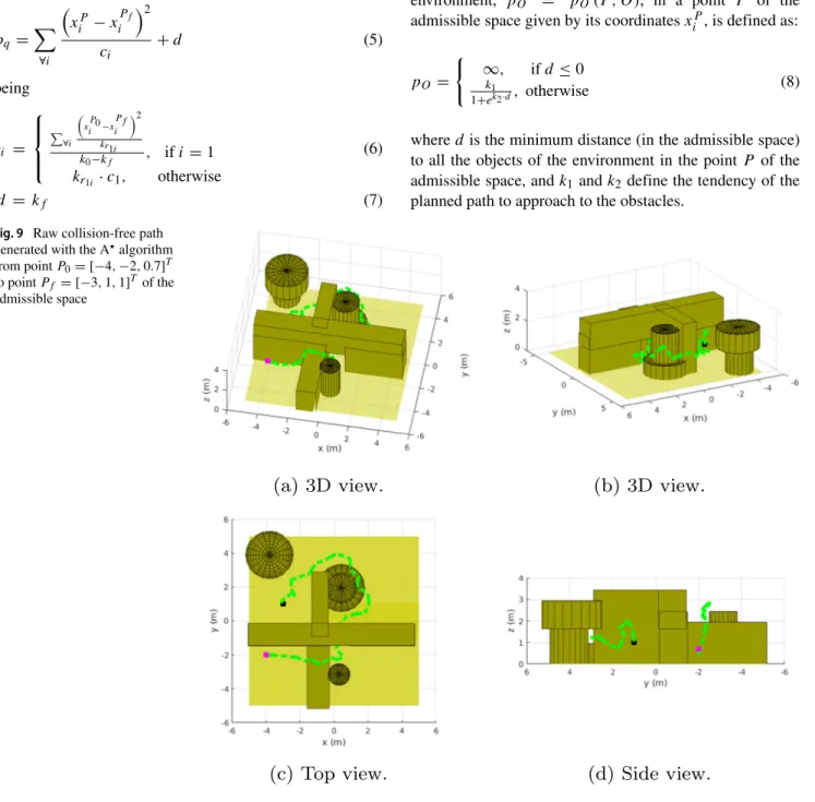
Fig. 9 Raw collision-free path generated with the Aalgorithm from pointP0=[−4,−2,0.7]T to pointPf =[−3,1,1]T of the admissible space
4.4.3 Cost of Moving Between Two Points
Given a potential field mapp, it generates a surfaceSgiven by S = [P , p (P )]T, for all points P of the admissible space.
The cost of moving between points A and B of the admissible space following the curveCA→B, is given by the
line integral for the unit scalar field along the curveCA→B,
that is the projection of the curveCA→Bover the surfaceS:
c (A, B)= CA→B 1· dl CA→B l (9)
where A = [A, p(A)]T, B = [B, p(B)]T, and dl =
[dt(P ),dp(P )]T, with dt(P )being the tangent vector of the curveCA→Bin the pointP.
If the curveCA→B is parametrized bys ∈ [smin, smax],
then, any pointP of this curve is given bytP(s), and for a s=si−si−1: l= t p = tP(si)−tP(si−1) p (tP(si))−p (tP(si−1)) (10)
and sampling the s interval, the cost of moving between points A and B, is calculated combining Eqs. 9 and 10, getting: c (A, B) smax si=smin t2+ p2 (11)
In the case that the curve, CA→B is a straight line
connecting pointsAandB, the following parametrization can be used:
s∈[smin, smax]=
0,tPB −tPA (12)
being a generic point P of the admissible space over the curveCA→Bgiven by:
tP(s)=tPA+s·nC (13)
where
nC= tPB −tPA tPB −tPA
(14)
Fig. 10 Shortened collision-free path (in red) from point
P0=[−4,−2,0.7]T to point
Pf =[−3,1,1]T of the admissible space
Fig. 11 Shortened collision-free path from the initial position of the robot to the goal
tfWR =[−3,1,1]T in the work space
and for as=si−si−1:
t=s·nC (15)
and therefore, sampling thes interval, the cost of moving between pointsAandB, is calculated by:
c (A, B) smax si=0 s2+(p (tP(s i))−p (tP(si−1)))2 (16) The number of sampling points of thes interval,nsi, is
calculated taken into account that theshas to be smaller than the smallest dimension of all the obstacles, and hence, at least a sampling point will fall inside the obstacle if it is crossed.
4.5 Graph Search Algorithm
Whenever the planner receives a planning query, it uses a simple but efficient widely used A algorithm, [7], to find the minimum cost path that connects the initial (current), P0, and desired state, Pf, in the probabilistic graph. This
informed search algorithm searches among all possible
paths to the solution for the one that incurs in the smallest cost, and among these paths, it first considers the ones that appear to lead most quickly to the solution. At each iteration of its main loop, it needs to determine which of its partial
Fig. 12 V-REP simulation environment. Static objects are colored as silver, while moving objects are colored as red (aerial) and yellow (ground)
Fig. 13 Simulation experiment att=0 s. The aerial robot is represented with a purple cylinder, the static objects are depicted in gray, and the moving objects in turquoise. The planned collision-free path is represented by a dashed red line, whereas the followed path is a solid blue line
path to expand into one or more longer paths. It selects the path that minimizes:
f (Pi)=g(P0, Pi)+h(Pi, Pf) (17)
wherePi is the working node of the graph on the current
iteration,g(P0, Pi)is the smallest cost of the path from node
P0to nodePiin the probabilistic graph, andh(Pi, Pf)is an
heuristic that estimates the cheapest path from nodePi to
nodePf in a straight line in the admissible space.
To guide the A algorithm during the search task, and to incorporate the knowledge of the obstacles of the environment, the cost function defined in Section4.4based on the potential field map, is used.
The costg(P0, Pi)is given by the sum of the cost needed
to move between nodeP0and nodePiin the probabilistic
graph:
g(P0, Pi)= Pj+1=Pi
Pj=P0
cPj, Pj+1 (18)
where the cost functioncPj, Pj+1
incorporates the contri bution to the potential field map of the query and the obstacles. The heuristic costh(Pi, Pf)is given by the cost needed
to move from nodePito nodePf in a straight line in the
admissible space:
h(Pi, Pf)=cPi, Pf (19)
where the cost function cPi, Pf only incorporates the
contribution to the potential field map of the query (but not the obstacles).
After the exploration of the graph, the path, tr, (also
called plan) has to be created by revisiting the explored nodes. The raw collision-free path computed by the A algorithm in the previous example can be seen in Fig.9. 4.6 Path Shortening
Once a collision-free path, tr, has been found by the A
algorithm, a post-processing is applied to shorten it to ts.
Fig. 15 Simulation experiment att=9.7 s. For a detailed figure description, please refer to Fig.13
Figure 10 shows the shortened path of the previous example in the admissible space, whereas Fig.11shows the shortened path in the work space.
The initial node,P0, and the final node,Pf, are always
the beginning and ending points of the shortened path. The middle points of the shortened path are calculated following Algorithm 1. In this algorithm, the path is shortened taking only into account the contribution to the potential field map of the obstacles of the environment (but not the query).
Algorithm 1Path shortening algorithm
Initialization:ts = {},Pi=P0,Pj =Pi+1 Loop: whilePj =Pf,∀Pj ∈tr do ifcPi, Pj ≥Pk+1=Pj Pk=Pi c (Pk, Pk+1)then ts = {ts, Pj},Pi←Pj end if Pj ←Pj+1 end while ts = {ts, Pf}
Note: The cost functioncPi, Pjincorporates only the
contribution to the potential field map of the obstacles.
5 Path Planner Additional Functionalities
Besides the collision-free path generation service (described in Section 4), the path planner component presented in Section 3, provides two key additional functionalities described along this section: the collision-free path check action (Section 5.1), and the better collision-free path generation service (Section5.2).
5.1 Collision-Free Path Check
The planned collision-free path, ts, has to be checked
whenever the environment changes to determine if it is still collision-free. The cost of the already planned collision-free pathts is calculated by:
c(P0, Pf)= Pj+1=Pf Pj=P0 cPj, Pj+1 (20) where the cost function cPj, Pj+1
corresponds to the potential field map, incorporating only the contribution of the obstacles. The path is considered to be collision-free, if its cost is lower than a threshold. Otherwise, it needs to be replanned.
5.2 Better Collision-Free Path Generation
As the environment is constantly changing, the previously planned collision-free path,ts, despite being collision-free,
might not be the most optimal in terms of cost.
To overcome this fact, the better collision-free path generation service has been developed. This service, executes the collision-free path generation service as described in Section 4, but keeping the previously planned path. Then, using Eq. 20, the cost of both candidate collision-free paths is computed. If the new collision-free path has a strictly lower cost than the previous path, it is returned as a better collision-free path, otherwise, the previous path is considered as the most optimum one.
6 Evaluation and Results
This section presents the methodology and evaluation of the proposed path planning solution.
Fig. 16 Simulation experiment att=11.8 s. For a detailed figure description, please refer to Fig.13
6.1 Methodology
The proposed path planning solution is implemented in C++ using the Robot Operative System (ROS), [28], as middleware. The path planning solution has been integrated into dif-ferent fully autonomous multi-rotor aerial robotic systems with the aim to evaluate its performance within a com-plete system. To achieve a fully autonomous operation, a large number of additional components, which are out of the scope of this paper, have been used. These additional components are: perception and state estimation, Sanchez-Lopez et al. [35], Bavle et al. [4]; control, Pestana et al. [24], Olivares-Mendez et al. [23]; mission plan specifica-tion, Molina et al. [19,20]; multi-robot mission planning, Sampedro et al. [31]; and human-machine interfaces, Su´arez Fern´andez et al. [40], among others.
Moreover, the path planning solution has also been integrated in the open-source framework for aerial robotics Aerostack, Sanchez-Lopez et al. [33,36], although only the 2D version has been released as open-source code.
Nevertheless, having a working situation awareness system for a dynamic 3D environment, is still an open problem that the scientific community is currently tackling, which limits the validation scope of the proposed path planning solution.
Simulations of fully autonomous multi-rotor aerial robots performing in highly challenging dynamic environments are presented in Section 6.2. In these simulations, scenes are formed by a complex static environment in combination with a large number of moving objects. Dynamic models of different multi-rotor aerial robots have been included in these scenes. Using the above-mentioned different components, the simulated multi-rotor aerial robots are required to navigate in these scenes fully autonomously. At the end of this section, the simulation results are evaluated.
To complement the simulations, Section 6.3 presents the previous usages of the 2D version of the proposed path planning solution in a fully autonomous aerial robotic system, and discusses the difficulty found on the validation of the presented 3D version.
Fig. 18 Simulation experiment att=20.45 s. For a detailed figure description, please refer to Fig.13
6.2 Simulations in Dynamic Environments
The proposed path planner has been evaluated by means of realistic simulations. The simulations were carried out using the V-REP simulator, [30], with different scenes as the one shown in Fig.12.
For the sake of brevity, only one simulation is presented in this paper, but a complimentary set of simulations can be found online.1
The presented simulation is carried out in an environment of 15×15×4= 900 m3, using a DJI M100 like aerial robot platform (approx. 40 cm of radius and a height of 40 cm). The used scene, shown in Fig. 12, incorporates multiple static objects, colored as silver, some of them forming a house with a door-like aperture, and two Velux-like roof openings. The scene incorporates four ground moving objects (colored as yellow) as well with cylindrical and prism shape, and six cylinder-shaped aerial moving objects (colored as red). The apertures of the house are occasionally blocked by the moving objects. The aerial moving objects have been incorporated to increase the complexity of the navigation, as the ground moving objects can be easily avoided by flying above them. The complete information of the situation, both of the robot and the objects of the environment, is received directly from the simulator.
The aerial robot takes off behind two walls outside the house at initial positionP0=[−5.525,−6.625,1]T, and it is requested to reach goal positionPf = [5.0,5.0,0.7]T,
which is located inside the house.
The configuration parameters of the path planning solution are the following:
1Complimentary set of simulations: (i.e.https://youtu.be/4zMjwlbD2P8)
– Admissible space: threshold distance to ignore the moving objects,dO=5.0 (m in the admissible space).
– Probabilistic graph: number of nodes,n=5500, with a 6-neighborhood (6.11 nodes/m3).
– Potential field map of the planning query:kr1y = 1.0,
kr1y=3.0,k0=1.0·10
6, andk
f =0.0.
– Potential field map of the obstacles:k1=1.0·106, and k2=2.5.
– Path check: distance of loosing the path,dt =0.6.
– Better path generation: period on requesting a better path,Tbet ter =1.0·tplanning(s), wheretplanningis the
time (in seconds) that the path planner needed to plan the previously planned collision-free path.
The simulation starts att =0 s, once the aerial robot is hovering in the air, and the goal is sent to the path planning system. As shown in Fig.13, the planned collision-free path climbs up the walls that are outside the house and enters the house through the right roof opening.
As soon as the aerial robot advances following the path, some of the mobile obstacles are located within the distance rangedO of the robot, therefore, they are considered in the
admissible space. The collision-free path is subsequently adapted, as can be seen in Fig.14.
In Fig.15, the moving obstacle entered in the previously planned collision-free path, which forced the planner to generate a new collision-free path by flying over the moving obstacle.
Figure 16 shows a new better collision-free path that the planner has found while it is moving toward the goal, adapting the path to the changes of the dynamic environment.
In Fig.17, the aerial robot is passing by a moving object. Figure18shows the exact time instant where the aerial robot is targeting the roof opening and is ready to descend to enter the house.
Fig. 19 Simulation experiment att=23.35 s. For a detailed figure description, please refer to Fig.13 The aerial robot crosses the roof opening att =23.35 s,
as shown in Fig.19.
Finally, in Fig. 20, the aerial robot safely reached the goal inside the house after having avoided all the possible collisions and adapted its behaviors with respect to the dynamic obstacles presence in the environment.
Despite the high complexity of the simulations, incor-porating complex static obstacles, and multiple dynamic objects, the proposed path planner is capable of performing in real-time within a fully autonomous system, and generat-ing collision-free paths to reach complex goals (this could never have been reached using only a reactive approach), adapting them to the changes in the environment due to dynamic obstacles.
6.3 Real Flights in Dynamic Environments
Validation of the proposed path planning solution requires not only simulations but also real flights of the fully autonomous aerial robotic system.
The previous version of the here proposed path planner, described in Sanchez-Lopez et al. [37], has been validated
thanks to its intensive usage in multiple research projects, including three international competitions, IMAV 2013, Pestana et al. [25, 27], IARC 2014, Sanchez-Lopez et al. [26], and IMAV 2016; and in several applications for search and rescue (see Fig.21), exploration, and inspection applications among others, Sanchez-Lopez et al. [32, 33], Sampedro et al. [31], Sanchez-Lopez et al. [34, 36]. Its performance has been demonstrated in applications where multiple aerial robot agents are used as moving obstacles, while in others human beings are employed. In all these usages, the planner was able to calculate feasible collision-free paths with real-time operation, generating new paths fast enough when necessary.
Nevertheless, it is a highly challenging task to validate the newly added 3D navigation capabilities of the proposed path planner with a real fully autonomous aerial robotic system. It requires not only a 3D test area available, but also additional components for perception, control, mission planning, etc., that are out of the scope of this paper. As stated before, having a working situation awareness system for a dynamic 3D environment is still an open problem that the scientific community is currently tackling. This makes
Fig. 21 Real flight experiment of [36], using the previous version of the here presented path planning solution for a multi-robot search and rescue application
the full validation of the proposed path planner with a real flight highly challenging, and this will remain as a future work.
7 Conclusions and Future Work
In this paper, we have presented a real-time collision-free path planning solution for 3D navigation of multi-rotor aerial robots in complex dynamic environments, which is an extension of our previous work, [37].
Our path planner represents the situation, including the self-situation and the situation of the environment, with high-level geometric primitives, unlike other less compact descriptions using grid maps or octrees. The admissible space, where the optimal solution has to be searched, is gen-erated incorporating novel concepts imported from control theory. It is sampled at launching time utilizing a prob-abilistic graph. Unlike other widely known probprob-abilistic approaches such as PRM, this probabilistic graph does not incorporate the information of existing objects in the envi-ronment. Whenever a planning query is received, an A discrete search algorithm is employed to explore the prob-abilistic graph in order to find a raw optimal collision-free path (subsequently shortened), which therefore guarantees the optimality of, if any exists, the obtained collision-free path. To include the information of existing obstacles in the environment without modifying the probabilistic graph (what is computationally expensive), an artificial potential field map is employed as the cost function of the discrete search algorithm. Unlike typical implementations of arti-ficial potential field maps, our planner always finds an
optimal path without dropping into local minima. These key features of the proposed path planning algorithm enable its real-time operation in complex dynamic environments.
The proposed path planning solution has been integrated within a complete fully autonomous robotic system for its evaluation. It has been fully evaluated by means of realistic simulations using the V-REP simulator in complex environments with multiple moving objects.
The evaluation results support that the proposed path planning solution is capable of performing in real-time within a fully autonomous system, generating collision-free paths to reach complex goals, and adapting them to the changes of the environment due to the dynamic obstacles.
Our future work lines mainly include evaluation of other discrete search algorithms which are potentially more suitable for dynamic environments, such as the D, Stentz [39], implementation of more complex high-level geometric primitives to represent the situation, and development of newer shortening algorithms to obtain a smoother path.
Moreover, an important limitation of the proposed path planner is the need of sampling admissible space at launching time. This limitation disqualifies the planner for exploration usage and limits its performance when the number of nodes is insufficient. To overcome this limitation, algorithms such as a Lazy-PRM, Bohlin and Kavraki [5], or a C-PRM, Song et al. [38], might be used for further improvement of the proposed solution. In addition, higher dimensional search spaces (including, for example, heading and velocity) should be implemented in the future work. Finally, validation of our proposed path planning solution by means of real flights has to be completed by developing adequate situation awareness components.
Acknowledgments This work was supported by the “Fonds National de la Recherche” (FNR), Luxembourg, under the project C15/15/10484117 (BEST-RPAS).
Publisher’s Note Springer Nature remains neutral with regard to jurisdictional claims in published maps and institutional affiliations.
References
1. (2017) ROS navigation stack.http://wiki.ros.org/navigation
2. Aguiar, A.P., Hespanha, J.P.: Trajectory-tracking and path-following of underactuated autonomous vehicles with parametric modeling uncertainty. IEEE Trans. Autom. Control52(8), 1362– 1379 (2007).https://doi.org/10.1109/TAC.2007.902731
3. Arantes, M.d.S., Arantes, J.d.S., Toledo, C.F.M., Williams, B.C.: A hybrid multi-population genetic algorithm for UAV path planning. In: Proceedings of the 2016 on Genetic and Evolutionary Computation Conference, pp. 853–860. ACM (2016)
4. Bavle, H., Sanchez-Lopez, J.L., Rodriguez-Ramos, A., Sampedro, C., Campoy, P.: A flight altitude estimator for multirotor UAVS in dynamic and unstructured indoor environments. In: 2017 International Conference on Unmanned Aircraft Systems (ICUAS), pp. 1044–1051 (2017).https://doi.org/10.1109/ICUAS. 2017.7991467
5. Bohlin, R., Kavraki, L.E.: Path planning using lazy prm. In: Proceedings 2000 ICRA. Millennium Conference. IEEE International Conference on Robotics and Automation. Symposia Proceedings (Cat. No.00CH37065), vol. 1, pp. 521–528 (2000).
https://doi.org/10.1109/ROBOT.2000.844107
6. Chen, Y.B., Luo, G.c., Mei, Y.s., Yu, J.q., Su, X.l.: UAV path planning using artificial potential field method updated by optimal control theory. Int. J. Syst. Sci.47(6), 1407–1420 (2016) 7. Dechter, R., Pearl, J.: Generalized best-first search strategies and
the optimality of a*. J. ACM32(3), 505–536 (1985).https://doi. org/10.1145/3828.3830
8. Hart, P.E., Nilsson, N.J., Raphael, B.: A formal basis for the heuristic determination of minimum cost paths. IEEE Trans. Syst. Sci. Cybern.4(2), 100–107 (1968)
9. Holland, J.H.: Adaptation in Natural and Artificial Systems: an Introductory Analysis with Applications to Biology, Control, and Artificial Intelligence. MIT Press (1992)
10. Hossain, M.A., Ferdous, I.: Autonomous robot path planning in dynamic environment using a new optimization technique inspired by bacterial foraging technique. Robot. Auton. Syst.64, 137–141 (2015)
11. Hwang, Y.K., Ahuja, N.: A potential field approach to path planning. IEEE Trans. Robot. Autom. 8(1), 23–32 (1992).
https://doi.org/10.1109/70.127236
12. Kassim, A.A., Kumar, B.V.: A neural network architecture for path planning. In: International Joint Conference on Neural Networks, 1992. IJCNN, vol. 2, pp. 787–792. IEEE (1992) 13. Kavraki, L.E., Svestka, P., Latombe, J.C., Overmars, M.H.:
Probabilistic roadmaps for path planning in high-dimensional configuration spaces. IEEE Trans. Robot. Autom.12(4), 566–580 (1996).https://doi.org/10.1109/70.508439
14. Kennedy, J.: Particle swarm optimization. In: Encyclopedia of machine learning, pp. 760–766. Springer (2011)
15. Lacasa, L., Luque, B., Ballesteros, F., Luque, J., Nuno, J.C.: From time series to complex networks: the visibility graph. Proc. Natl. Acad. Sci.105(13), 4972–4975 (2008)
16. LaValle, S.M.: Rapidly-Exploring Random Trees: a New Tool for Path Planning. Citeseer (1998)
17. Lin, Y., Saripalli, S.: Sampling-based path planning for UAV collision avoidance. IEEE Trans. Intell. Transp. Syst. (2017) 18. Liu, S., Atanasov, N., Mohta, K., Kumar, V.: Search-based motion
planning for quadrotors using linear quadratic minimum time control. arXiv:170905401(2017)
19. Molina, M., Diaz-Moreno, A., Palacios, D., Suarez-Fernandez, R.A., Sanchez-Lopez, J.L., Sampedro, C., Bavle, H., Campoy, P.: Specifying complex missions for aerial robotics in dynamic environments. In: International Micro Air Vehicle Conference and Competition, IMAV, p. 2016, Beijing (2016)
20. Molina, M., Suarez-Fernandez, R.A., Sampedro, C., Sanchez-Lopez, J.L., Campoy, P.: Tml: a language to specify aerial robotic missions for the framework aerostack. Int. J. Intell. Comput. Cybern.10(4), 491–512 (2017). https://doi.org/10.1108/IJICC-03-2017-0025
21. Narayanan, V., Phillips, M., Likhachev, M.: Anytime safe interval path planning for dynamic environments. In: 2012 IEEE/RSJ International Conference on Intelligent Robots and Systems (IROS), pp. 4708–4715. IEEE (2012)
22. Nieuwenhuisen, M., Droeschel, D., Beul, M., Behnke, S.: Autonomous navigation for micro aerial vehicles in complex
gnss-denied environments. J. Intell. Robot. Syst.84(1–4), 199– 216 (2016)
23. Olivares-Mendez, M., Kannan, S., Voos, H.: Vision based fuzzy control autonomous landing with UAVS: from V-REP to real experiments. In: 2015 23th Mediterranean Conference on Control and Automation (MED), pp. 14–21 (2015).
https://doi.org/10.1109/MED.2015.7158723
24. Pestana, J., Mellado-Bataller, I., Sanchez-Lopez, J.L., Fu, C., Mondrag´on, I.F., Campoy, P.: A general purpose configurable controller for indoors and outdoors gps-denied navigation for multirotor unmanned aerial vehicles. J. Intell. Robot. Syst.73(1), 387–400 (2014).https://doi.org/10.1007/s10846-013-9953-0
25. Pestana, J., Sanchez-Lopez, J.L., de la Puente, P., Carrio, A., Cam-poy, P.: A vision-based quadrotor swarm for the participation in the 2013 international micro air vehicle competition. In: Inter-national Conference on Unmanned Aircraft Systems (ICUAS), pp. 617–622 (2014).https://doi.org/10.1109/ICUAS.2014.6842305
26. Pestana, J., Collumeau, J.F., Suarez-Fernandez, R., Campoy, P., Molina, M.: A vision based aerial robot solution for the mission 7 of the international aerial robotics competition. In: 2015 Inter-national Conference on Unmanned Aircraft Systems (ICUAS), pp. 1391–1400 (2015).https://doi.org/10.1109/ICUAS.2015.7152 435
27. Pestana, J., Sanchez-Lopez, J.L., de la Puente, P., Carrio, A., Campoy, P.: A vision-based quadrotor multi-robot solution for the indoor autonomy challenge of the 2013 international micro air vehicle competition. J. Intell. Robot. Syst.84(1), 601–620 (2016).
https://doi.org/10.1007/s10846-015-0304-1
28. Quigley, M., Conley, K., Gerkey, B., Faust, J., Foote, T., Leibs, J., Wheeler, R., Ng, A.Y.: Ros: an open-source robot operating system. In: ICRA Workshop on Open Source Software, vol. 3, p. 5 (2009)
29. Richter, C., Bry, A., Roy, N.: Polynomial Trajectory Planning for Aggressive Quadrotor Flight in Dense Indoor Environments, pp. 649–666. Springer International Publishing, Cham (2016) 30. Rohmer, E., Singh, S.P.N., Freese, M.: V-rep: a versatile and
scalable robot simulation framework. In: IEEE/RSJ International Conference on Intelligent Robots and Systems, pp. 1321–1326 (2013).https://doi.org/10.1109/IROS.2013.6696520
31. Sampedro, C., Bavle, H., Sanchez-Lopez, J.L., Su´arez Fern´andez, R.A., Rodr´ıguez-Ramos, A., Molina, M., Cam-poy, P.: A flexible and dynamic mission planning architecture for UAV swarm coordination. In: International Conference on Unmanned Aircraft Systems (ICUAS), pp. 355–363 (2016).
https://doi.org/10.1109/ICUAS.2016.7502669
32. Sanchez-Lopez, J.L., Pestana, J., de la Puente, P., Suarez-Fernandez, R., Campoy, P.: A system for the design and devel-opment of vision-based multi-robot quadrotor swarms. In: Inter-national Conference on Unmanned Aircraft Systems (ICUAS), vol. 2014, pp. 640–648 (2014).https://doi.org/10.1109/ICUAS.2014.
33. Sanchez-Lopez, J.L., Pestana, J., de la Puente, P., Campoy, P.: A reliable open-source system architecture for the fast designing and prototyping of autonomous multi-UAV systems: simulation and experimentation. J. Intell. Robot. Syst.84(1), 779–797 (2016).
https://doi.org/10.1007/s10846-015-0288-x
34. Sanchez-Lopez, J.L., Su´arez Fern´andez, R.A., Bavle, H., Sampedro, C., Molina, M., Pestana, J., Campoy, P.: Aerostack: an architecture and open-source software frame-work for aerial robotics. In: International Conference on Unmanned Aircraft Systems (ICUAS), pp. 332–341 (2016).
https://doi.org/10.1109/ICUAS.2016.7502591
35. Sanchez-Lopez, J.L., Arellano-Quintana, V., Tognon, M., Cam-poy, P., Franchi, A.: Visual marker based multi-sensor fusion state estimation. In: Proceedings of the 20th IFAC World Congress (2017)
36. Sanchez-Lopez, J.L., Molina, M., Bavle, H., Sampedro, C., Su´arez Fern´andez, R.A., Campoy, P.: A multi-layered component-based approach for the development of aerial robotic systems: the aerostack framework. J. Intell. Robot. Syst.
https://doi.org/10.1007/s10846-017-0551-4(2017)
37. Sanchez-Lopez, J.L., Pestana, J., Campoy, P.: A robust real-time path planner for the collision-free navigation of multirotor aerial robots in dynamic environments. In: 2017 International Conference on Unmanned Aircraft Systems (ICUAS), pp 316– 325.https://doi.org/10.1109/ICUAS.2017.7991354(2017) 38. Song, G., Miller, S., Amato, N.M.: Customizing prm roadmaps at
query time. In: Proceedings 2001 ICRA. IEEE International Confe-rence on Robotics and Automation (Cat. No.01CH37164), vol 2., pp. 1500–1505https://doi.org/10.1109/ROBOT.2001.932823(2001) 39. Stentz A: Optimal and efficient path planning for partially-known environments. In: Proceedings of the 1994 IEEE International Conference on Robotics and Automation. Proceedings, vol. 4, pp. 3310–3317 (1994).https://doi.org/10.1109/ROBOT.1994.351 061
40. Su´arez Fern´andez, R.A., Sanchez-Lopez, J.L., Sampedro, C., Bavle, H., Molina, M., Campoy, P.: Natural user interfaces for human-drone multi-modal interaction. In: International Conference on Unmanned Aircraft Systems (ICUAS), vol. 2016, pp. 1013– 1022 (2016).https://doi.org/10.1109/ICUAS.2016.7502665
41. Tisdale, J., Kim, Z., Hedrick, J.K.: Autonomous UAV path planning and estimation. IEEE Robot. Autom. Mag.16(2) (2009) 42. Wurm, K.M., Hornung, A., Bennewitz, M., Stachniss, C., Burgard, W.: Octomap: A probabilistic, flexible, and compact 3d map representation for robotic systems. In: Proceedings of the ICRA 2010 Workshop on Best Practice in 3D Perception and Modeling for Mobile Manipulation, vol 2 (2010)
43. Yan, F., Liu, Y.S., Xiao, J.Z.: Path planning in complex 3d environments using a probabilistic roadmap method. Int. J. Autom. Comput.10(6), 525–533 (2013)
44. Yang, L., Qi, J., Song, D., Xiao, J., Han, J., Xia, Y.: Survey of robot 3d path planning algorithms. J. Control Sci. Eng.2006, 5 (2016) 45. Yao, P., Wang, H., Liu, C.: 3-d dynamic path planning for UAV
based on interfered fluid flow. In: Guidance, Navigation and Control Conference (CGNCC), IEEE Chinese, pp. 997–1002. IEEE (2014)
46. Yue, R., Xiao, J., Wang, S., Joseph, S.L.: Modeling and path planning of the city-climber robot part ii: 3d path planning using mixed integer linear programming. In: 2009 IEEE International Conference on Robotics and Biomimetics (ROBIO), pp. 2391– 2396. IEEE (2009)
Jose Luis Sanchez-Lopez is a post-doctoral research associate at Automation & Robotics Research Group of the Interdisciplinary Centre for Security Reliability and Trust (SnT) of the University of Luxembourg (since June 2017).
He received his Ph. D. in Robotics (May 2017), his Master degree in Automation and Robotics (Oct. 2012), and his Engineering degree in Industrial Engineering (Sep. 2010), at the Technical University of Madrid.
He was a visiting researcher during six months (Jul. – Dec. 2012) at Arizona State University (AZ, USA), and during thirteen months (Sep. – Dec 2014 & Nov. 2015 – Oct. 2016) at LAAS-CNRS (Toulouse, France).
His main research goal is to provide robots, with a special focus on aerial robots, with the maximum level of autonomy allowing them to perform different missions without human intervention. His research interests comprise intelligent and cognitive system architectures, multi-agent systems, sensor fusion and state estimation, localization and mapping, trajectory and path planning, computer vision and machine learning. He has authored more than 35 publications related to these fields.
Min Wangis a Ph.D. candidate at the Interdisciplinary Centre for Security Reliability and Trust (SnT) of the University of Luxembourg since February 2017. She received her M.S. in Robotics Engineering from University of Genoa and Warsaw University of Technology in 2013, and her B.E.in Automation from Wuhan University of Technology in 2011. Her main research interests include sensing, computer vision, machine learning and robotics.
Miguel A. Olivares-Mendezreceived the Diploma in Computer Sci-ence Engineering in 2006 from the University of Malaga (UMA), Spain. He received the M.Sc. degree in Robotics and Automation and PhD degree in Robotics and Automation at the Industrial Engineering Faculty in the Technical University of Madrid (UPM), Spain, in 2009 and 2013, respectively. He was distinguished with the Best PhD Thesis award of 2013 by the European Society for Fuzzy Logic and Technol-ogy (EUSFLAT). He joined the Interdisciplinary Center for Security Reliability and Trust (SnT) at the University of Luxembourg on May 1, 2013, as Associate Researcher in the Automation and Robotics Research Group. Since May 1, 2013, he is acting as Associate Editor for Journal of Intelligent & Robotic Systems (JINT). In December 1, 2015, he was selected to be Reviewer Editor for the Robotic Control Systems, part of the journal(s) Frontiers in Robotics and AI.
Dr. Olivares-Mendez’s research interests are focused in the areas of Unmanned Systems, Computer Vision, Vision-Based Control, Soft-Computing Control Techniques, Fuzzy control, Sensor Fusion, Robotics and Automation. He has been working in robotics and control with unmanned systems since 2006. He has published over 50 book chapters, technical journals and referred conference papers.
Martin Molinais a professor at the Department of Artificial Intel-ligence, Technical University of Madrid since 1994 (full professor since 2012). He received his Ph.D. in computer science and arti-ficial intelligence in 1993 and his licentiate degree in information technology in 1990 from the Technical University of Madrid (UPM). He was a visiting researcher for approximately 3 years in several research centers in the USA (AT&T LabsResearch, Stanford Univer-sity and UniverUniver-sity of California-Irvine). Martin Molina led a research group about intelligent systems at his university (1999-2016). Cur-rently, Martin Molina is a member of the research group Computer Vision and Aerial Robotics at UPM, where he leads research lines related to artificial intelligence methods applied to aerial robotics (e.g., cognitive architectures, human-machine interaction, agent-based architectures, and machine learning). He has been the principal inves-tigator of 26 research projects and he has authored more than 90 publi-cations related to artificial intelligence. He has more than 20 years of experience working with intelligent systems and their practical applica-tions with an important relation with private companies related to engineering problems (robotics, transport, hydrology, aeronautics, etc.).
Holger Voosstudied Electrical Engineering at the Saarland University and received the Doctoral Degree in Automatic Control from the Technical University of Kaiserslautern, Germany, in 2002. From 2000 to 2004, he was with Bodenseewerk Ger¨atetechnik GmbH, Germany, where he worked as a Systems Engineer in aerospace and robotics. From 2004 to 2010, he was a Professor at the University of Applied Sciences Ravens-burg-Weingarten, Germany, and the head of the Mobile Robotics Lab there. Since 2010, he is a Professor at the University of Luxembourg in the Faculty of Science, Technology and Communication, Research Unit of Engineering Sciences. He is the head of the Au-tomation and Robotics Research Group in the Interdisciplinary Centre of Security, Relia-bility and Trust (SnT) at the University of Luxembourg. His research interests are in the area of sensing and control for autonomous vehicles and robots as well as distributed and networked control and automation.
![Fig. 6 Admissible space of the example presented in Fig. 2. The robot is located in the point P 0 = [−4, −2, 0.7] T](https://thumb-us.123doks.com/thumbv2/123dok_us/10952153.2983721/8.892.256.815.561.1090/fig-admissible-space-example-presented-robot-located-point.webp)
![Fig. 10 Shortened collision-free path (in red) from point P 0 = [−4, −2, 0.7] T to point P f = [−3, 1, 1] T of the admissible space](https://thumb-us.123doks.com/thumbv2/123dok_us/10952153.2983721/12.892.107.824.393.1085/fig-shortened-collision-free-point-point-admissible-space.webp)