EPIC: A NEW AND ADVANCED NONLINEAR PARABOLIZED STABILITY EQUATION SOLVER
A Thesis by
NICK BRANDON OLIVIERO
Submitted to the Office of Graduate and Professional Studies of Texas A&M University
in partial fulfillment of the requirements for the degree of MASTER OF SCIENCE
Chair of Committee, Helen L. Reed
Committee Members, Rodney D. W. Bowersox Hamn-Ching Chen Head of Department, Rodney D. W. Bowersox
May 2015
Major Subject: Aerospace Engineering
ABSTRACT
Recent years have witnessed the linear and nonlinear parabolized stability equations (PSE) become a quintessential component toward understanding boundary-layer laminar-to-turbulent transition. Because of the abundant benefits an accurate and trustworthy computational analysis can provide, wind tunnel experiments are commonly supplemented with such studies. Prompted by the rising need to develop a fast, modern, intuitive, and user-friendly PSE code, this work describes the development, validation, and verification of EPIC.
EPIC is a new Nonlinear Parabolized Stability Equation (NPSE) solver developed in-house in our Computational Stability and Transition (CST) lab that will aid in the study, understanding, and prediction of laminar-to-turbulent boundary layer transition problems. This entirely new code is an improvement upon and is intended to replace CST’s prior NPSE solver, called JoKHeR. PSE results computed for the NASA Langley 93-10 flared cone, Purdue compression cone, and SWIFTER airfoil are compared and show successful agreement with published computational and experimental results. It is expected that further application of a physics-based approach such as EPIC will lead to more accurate prediction, smaller and more manageable uncertainties in design, and an improved fundamental understanding of the laminar-turbulent transition process that will lead to efficient control strategies.
ACKNOWLEDGEMENTS
I would not be where I am today without the help and support of many people. I am especially thankful for my committee chair and advisor, Dr. Helen Reed. Through her pivotal lectures on stability and perturbation techniques in the classroom and her insightful discussions and mentorship outside of it, I always felt encouraged and capable. Under her expert guidance, unending patience, and never-ending support I have learned and accomplished far more than I could have hoped for. I feel deeply indebted to her for providing me with this opportunity.
A very special thank you goes out to Dr. John Valasek, whom I had the privilege to work for as an undergraduate. Working for him in the Vehicle Systems and Controls Laboratory provided me with first hand exposure to graduate research. The opportunity to apply the aerospace knowledge I was learning into computational code provoked both skills to symbiotically flourish. Furthermore, Dr. Valasek was among the first to peak my interest in pursuing graduate school. I must also thank Kristi Shryock, my undergraduate advisor, for directing me toward Dr. Valasek when I misguidedly approached her about changing my major.
I would like to thank all of my past and current co-workers, Eddie Perez, Matthew Tufts, Travis Kocian, Alex Moyes, and Megan Heard, for their various help and support throughout the years. I hope that I have reciprocated that help and I thoroughly enjoyed working with all of you. I also want to express my gratitude for all of the experimental work performed by Dr. William Saric and his team, Dr. Jerrod Hofferth, Dr. Alex Craig, Dr. Tom Duncan, Dr. Brian Crawford, and David West. A special thank you goes to Dr. Joseph Kuehl. His multiple consultations and contributions to our group helped facilitate this undertaking and lead to its eventual success. I am extremely grateful for the daily work Colleen Leatherman and Rebecca Marianno perform to keep our lab operational.
AFOSR/NASA National Center for Hypersonic Research in Laminar-Turbulent Transition through grant 09-1-0341. Further funding was provided by AFOSR grant FA9550-14-1-0365. In addition, I thank Pointwise, Inc. for their gridding software, and the Texas Advanced Computing Center (TACC) for their super-computing resources.
Finally, I thank my family for the never-ending support and encouragement throughout the years. An extra thank you goes to my lovely fianc´ee, Christina Hulsey, for her extreme patience and understanding, especially during those infamous late nights.
NOMENCLATURE
VARIABLES
α Disturbance Streamwise Complex Wavenumber
β Disturbance Spanwise Complex Wavenumber
βAZ Azimuthal Beta
η Uniform Normal Grid;η∈[0,1]
γ Ratio of Specific Heats
κ Thermal Conductivity
λ Second Coefficient of Viscosity or Bulk Viscosity
µ Dynamic Coefficient Viscosity Ω Pressure Gradient Coefficient
ω Disturbance Frequency
∂ξ Step Size
Φ Eigenvector for LST; [ˆu; ˆv; ˆw; ˆT; ˆρ; ˆαu; ˆαv; ˆαw; ˆαT]
φ Flow variables [u, v, w, T, ρ]
Ψ Normalization Parameter Function
ρ Density
θki Disturbance Growth Direction
θk Phase Angle
ξ Uniform Streamwise Grid;ξ∈[Xs0, Xsend]
a Computational Normal Grid Coefficient
b Computational Normal Grid Coefficient
C1 Sutherland’s Law Constant
C2 Sutherland’s Law Constant
Cp Specific Heat for Constant Pressure
h1,h2,h3 Streamwise Marching, Wall Normal, and Spanwise Curvilinear Metric
Coefficient, respectively
i =√−1
L Boundary-Layer Reference Length
M Mach Number
N x Number of Streamwise Points
N y Number of Normal Points
P Pressure
P r Prandtl Number
Rc Radius of Curvature
Rg Specific Gas Constant
Re Reynolds Number
Sκ Sutherland’s κ Reference Constant
Sµ Sutherland’s µReference Constant
T Temperature
t Time
u,v,w Streamwise Marching, Wall Normal, and Spanwise Velocity, respectively
x,y,z Streamwise Marching, Wall Normal, and Spanwise Coordinate Direction, respectively
Xs Streamwise Surface Distance
ycrit Used to Determine Computational Normal Grid Clustering
yc Clustered Computational Normal Grid;yc∈[0, ymax]
Z Compressibility Factor SUBSCRIPTS
(n, k) Mode Number, wherenandkare integer coefficients of the fundamental
ω0 andβ0 respectively
0 Initial or Fundamental Value
i Imaginary Value
j The jth point of an array
r Real Value
SUPERSCRIPTS
0 Unsteady Disturbance Quantity
† Complex Conjugate
* Dimensional Value - Steady Basic-State Term
TABLE OF CONTENTS
Page
ABSTRACT . . . ii
ACKNOWLEDGEMENTS . . . iii
NOMENCLATURE . . . v
TABLE OF CONTENTS . . . viii
LIST OF FIGURES . . . x
LIST OF TABLES . . . xii
I. INTRODUCTION . . . 1
I.1 Historical Background . . . 1
I.2 Motivation and Objective . . . 8
I.3 Outline of Thesis . . . 9
II. GOVERNING EQUATIONS . . . 10
II.1 Coordinate System . . . 10
II.2 Basic-State Equations . . . 11
II.2.1 Thermodynamic Properties . . . 13
II.3 Nondimensionalization . . . 15
II.4 Disturbance Equations . . . 20
II.4.1 Boundary Conditions . . . 21
II.5 Disturbance Quantity Formulation . . . 21
II.5.1 Linear Stability Theory . . . 22
II.5.2 Linear Parabolized Stability Equations . . . 23
II.5.3 Nonlinear Parabolized Stability Equations . . . 25
III. NUMERICAL FORMULATION . . . 28
III.1 Computational Grid . . . 28
III.2 Finite-Difference Method . . . 30
III.3 Local Eigenvalue Solution . . . 31
III.4 Linear Marching Procedure . . . 32
III.4.1 Normalization Condition . . . 34
III.5 Nonlinear Marching Procedure . . . 35
III.5.2 Step Size Limitation . . . 37
III.6 Result Analysis Methods . . . 38
III.6.1 N-factor Analysis . . . 38
III.6.2 Amplitude Analysis . . . 39
IV. LANGLEY 93-10 RESULTS . . . 40
IV.1 Geometry . . . 40
IV.2 JoKHeR Verification . . . 44
IV.3 Validation . . . 49
V. PURDUE COMPRESSION CONE RESULTS . . . 51
V.1 Geometry . . . 51
V.2 LPSE Results and Validation . . . 52
V.3 Bandwidth NPSE Results . . . 54
VI. SWIFTER RESULTS . . . 58
VI.1 Geometry . . . 58
VI.2 LASTRAC Verification . . . 58
VII. SUMMARY . . . 60
REFERENCES . . . 62
APPENDIX A. BASIC-STATE EQUATIONS . . . 67
APPENDIX B. LST FORMULATION . . . 73
APPENDIX C. LPSE FORMULATION . . . 85
LIST OF FIGURES
FIGURE Page
II.1 Exaggerated visualization of curvilinear transformation. . . 12 IV.1 Langley 93-10 flared cone. . . 41 IV.2 Nose tip blended into straight portion of cone with modified super ellipse. . . 42 IV.3 Wall temperature distributions for the Langley 93-10 flared cone, showing the
experimental conditions in the M6QT [14], the adiabatic distribution, and the computational model of 398K. . . 43 IV.4 Langley 93-10 basic-state grid composed of two main parts in the wall normal
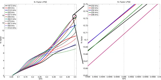
direction: a band capturing the shock and a high-resolution shock layer. . . . 44 IV.5 EPIC calculated LPSE N-factors for Langley 93-10 flared cone, featuring a
zoom at axial location x=0.495 m . . . 45 IV.6 JoKHeR calculated LPSE N-factors for Langley 93-10 flared cone, featuring a
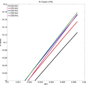
zoom at axial location x=0.495 m [19] . . . 45 IV.7 EPIC calculated LPSE N-Factors for Langley 93-10 flared cone, zoomed at
back of cone. . . 46 IV.8 JoKHeR calculated LPSE N-Factors for Langley 93-10 flared cone, zoomed at
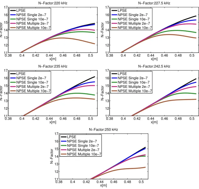
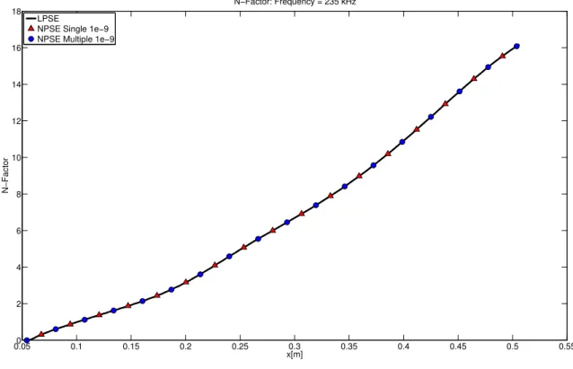
back of cone. . . 46 IV.9 Comparison of single and broadband NPSE for Langley 93-10 flared cone. Initial
amplitude given in terms of temperature perturbation. . . 48 IV.10 The single and multiple NPSE cases will recover the same solution as the LPSE
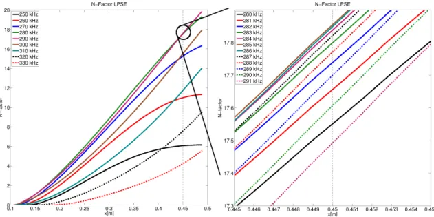
case if given a small enough initial amplitude. Initial amplitude given in terms of temperature perturbation. . . 49 V.1 Purdue compression cone. . . 51 V.2 EPIC calculated LPSE N-factors for Purdue Compression Cone, featuring a
zoom at axial location x=0.45 m . . . 52 V.3 Oblique mode LPSE N-Factors for Purdue compression cone . . . 53 V.4 Purdue compression cone oblique mode phase angles along axial distance . . . 53
V.5 LPSE N-Factors for streamwise counter-rotating streaks on Purdue compression cone. . . 53 V.6 First harmonic of EPIC calculated 1-, 3-, and 5-mode bandwidth NPSE
ampli-tudes for Purdue compression cone. . . 56 V.7 First harmonic of EPIC calculated 7-, 9-, and 11-mode bandwidth NPSE
amplitudes for Purdue compression cone. . . 56 V.8 Second harmonic of EPIC calculated 1-, 3-, and 5-mode bandwidth NPSE
amplitudes for Purdue compression cone. . . 57 V.9 Second harmonic of EPIC calculated 7-, 9-, and 11-mode bandwidth NPSE
amplitudes for Purdue compression cone. . . 57 VI.1 EPIC LPSE N-factors (colored lines) for SWIFTER wing glove with
LIST OF TABLES
TABLE Page
IV.1 Langley 93-10 flared cone validation comparisons . . . 50 V.1 Purdue compression cone validation comparisons . . . 54
I. INTRODUCTION
I.1 Historical Background
Edward Norton Lorenz, a chaos theory pioneer, once summarized his findings as ‘‘Chaos: When the present determines the future, but the approximate present does not approximately determine the future’’ [7]. Thus, it is fitting that while laminar flow is characterized by a smooth and uninterrupted stream, turbulent flow is its chaotic antithesis. As history has taught us, there could not be a more apt description of turbulence and its related processes than Lorenz’s own definition.
Though keen observers had previously documented the differences between laminar and turbulent flow, Osborne Reynolds was one of the first to publish about the phenomenon known as laminar-to-turbulent transition. In perhaps his most famous experiment, Reynolds studied water with streaks of color flowing through small glass tubes [38]. He observed that the colored bands remained in the given streak pattern under laminar flow conditions, but the streaks would diffuse and blend together under turbulent conditions. Reynolds noted during his tests that the resulting flow was not determined by just one property. By varying his initial flow conditions, Reynolds used a dimensionless quantity that combined all relevant flow properties, which he penned as Reynolds Number, to help predict flow characteristics. Reynolds noted the baseline criterion for when to expect laminar-to-turbulent transition to occur was anywhere between Re= 2000−13000 depending on how much care was given to the initial conditions.
While studying the same pipe flow as Reynolds (later coined as Poiseuille flow), William McFadden Orr [32, 33] and Arnold Sommerfeld [42] both independently developed what would eventually be known as the Orr-Sommerfeld equation. This equation attempted to prove that a critical Reynolds number could be solved for, suggesting that any portion of a flow could theoretically be determined as laminar or turbulent based on its characteristics. The Orr-Sommerfeld equation assumes that a small disturbance, possibly originating from
an irregularity in the flow or wall roughness, acts upon a laminar flow and can be modeled as a perturbation. If this perturbation is shown to grow, the flow is determined to be unstable and turbulence is assumed to occur. Despite intricate calculations, the problem would remain unsolved for a number of years.
In 1905, Ludwig Prandtl revolutionized the fluid mechanics field with his concept of the boundary layer. A boundary layer is the small fluid layer nearest to the surface that experiences substantial viscosity effects and is responsible for the majority of drag. Prandtl theorized that one could study the flow of a fluid by separating it into two layers. Viscosity was crucial for the flow within the boundary layer, but the outside layer could be treated as inviscid, vastly simplifying the Navier-Stokes equations associated with both flows. This revelation, however, did little more at the time than provide plausibility answers to many of the prevalent questions and paradoxes. The first mathematical application of the boundary layer was in 1908 when Prandtl’s first student, Paul Richard Heinrich Blasius, used it to justify solving the Navier-Stokes equations with an order-of-magnitude analysis [5]. The resulting Blasius boundary layer describes the steady, two-dimensional boundary layer of a semi-infinite flat plate parallel to a constant unidirectional flow.
After over a decade of studies in boundary-layer drag and turbulent flow characteristics, Prandtl and his doctoral student, Oskar Tietjans, presented their controversial findings at the Jena physics conference in 1921. Tietjans’ doctoral work had been the calculation of boundary layer motion with Rayleigh oscillations, but his findings contradicted previous presumptions. Thus far, all theories failed to yield a possible transition between laminar and turbulent flow, despite higher Reynolds numbers and experiments that proved the opposite. Prandtl and Tietjans’ calculations suggested that even the slightest disturbance at the lowest Reynolds number resulted in transition. Tietjans postulated that his theory failed because it was based on unrealistic velocity profiles composed of straight lines with arbitrary kinks. Shortly after this, Werner Heisenberg investigated the stability of the Poiseuille flow, a parabolic velocity profile between two parallel plates commonly observed in a pipe. Heisenberg’s doctoral thesis [10] provided a limit of stability, but his approximation
methods were impossible to justify at the time. Despite this, Prandtl was again motivated to solve the transition problem and he assigned a new dissertation topic to his next student, Walter Tollmien.
In 1929, Walter Tollmien completed his doctoral dissertation and produced the first successful stability phase diagram. By applying the Orr-Sommerfeld equation to the Blasius boundary layer profile, Tollmien could determine if a system was stable or unstable by the wavelength of the assumed disturbance and the Reynolds number of the flow. Hermann Schlichting expanded on Tollmien’s results by explicitly solving for the neutral stability location. He also extended Tollmien’s stability phase diagram to account for the pressure gradient of the profile, revealing that the unstable region would grow dramatically for an increasing positive pressure gradient. Finally, Schlichting determined that the onset of turbulence did not occur immediately upon entrance into the unstable region, but that it was dependent on the disturbance wave amplitude. The longer a disturbance wave remained in an unstable state, the more amplified it became, eventually reaching a high enough level to instigate turbulence. Based upon transition locations documented in experiments and his new stability phase diagrams, Schlichting calculated that the natural logarithm of amplitude ratio necessary for turbulence was about nine. This relation is commonly referred to as the N-factor or eN method, after van Ingen (1956) performed extensive calculations with it.
The theoretical results of Tollmien and Schlichting could not be proven until 1943 (published in 1947 after the war) when Schubauer and Skramstad confirmed their findings with experimental results [41]. Until this time, experiments had been conducted in wind tunnels with high free stream turbulence. By running their experiment in a new, low disturbance wind tunnel, Schubauer and Skramstad saw oscillatory waves as they grew downstream and broke down into turbulent flow. Their experimental agreement validated the linear stability theory efforts of the past 40 years and confirmed that the long-sought critical Reynolds number only determined where the transition would begin, as opposed to the transition location. The two-dimensional (2-D) waves theorized by Tollmien and
Schlichting and witnessed by Schubauer and Skramstad are now referred to as Tollmien-Schlichting waves, or TS waves.
The first attempt at a linear stability theory for compressible flow was made in 1938 by D. K¨uchemann, a student of none other than Walter Tollmien. Lester Lees and C.C. Lin followed this with a much more in depth application of linear stability theory on a compressible flow in 1946 (published 1947) [24]. Most of their report was focused on the inviscid theory, but an asymptotic viscous theory was included as well. Lees & Lin used a system of sixth-order ordinary differential equations and assumed locally parallel flow in order to derive two-dimensional disturbances in a perfect gas. These methods involved massive hand calculations, and thus disturbance amplitudes were not initially included. Through their results, Lees & Lin expanded upon Rayleigh’s inflection theory by confirming that a generalized inflection point (D(ρDU) = 0, where Dis ∂y∂ ,ρ is the density, andU
is the mean velocity) is a necessary and sufficient condition for neutral stability in a case where the phase speed is less than the freestream velocity. It was also falsely concluded that higher Mach numbers had a stabilizing effect on flows with an adiabatic-wall, based on the fact that the minimum critical Reynolds number decreased; the opposite was actually proved after the disturbance amplitudes were calculated.
The Dunn-Lin theory [8] attempted to develop a better viscous compressible stability theory by removing the largest restrictions from Lees & Lin’s theory: the idea that phase speed must be small and that disturbances could only be 2-D. However, the full 3-D stability equations resulted in a system of eighth-order ordinary differential equations that could not be reduced or solved at the time. To circumvent this, the Dunn-Lin theory drops the dissipation terms in the energy equation, thus permitting an order reduction by way of the Squire transformation. As pointed out by Dunn & Lin, this limits the validity of the their theory to studies below Mach 2.0. Their studies concluded that at speeds between Mach 1.0 and Mach 2.0, oblique 3-D disturbances begin to play a large role in the general instability of a boundary layer, most notably because they cannot be fully stabilized through wall cooling like the 2-D disturbances. Soon after, Reshotko [37] and Lees & Reshotko [25] were
able to add the dissipation terms back in to the theory, but they still relied on an asymptotic theory to obtain a final solution. These results produced strange multiple neutral curves at high Mach numbers and showed large discrepancies when compared with experimental results from Laufer and Vrebalovich [23].
The utilization of high speed computers in the 1960s finally allowed for direct solutions to linear stability theories. Mack’s in depth documentation of this is perhaps the most significant contribution to the stability problem in decades [29]. Mack thoroughly studied supersonic boundary-layer flows over flat plates at speeds up to Mach 10 and noted that supersonic boundary layer disturbances have unique features not seen in their subsonic counterparts. His initial direct solution results compared well to experimental values and confirmed that the asymptotic solution methods attempted by Dunn-Lin and Lees-Reshotko failed to produce accurate neutral stability curves above speeds of Mach 1.6.
Mack summarized his compressible linear stability findings as a couple of key points: 1) For all supersonic mean flows, the first mode is most unstable as an oblique wave, or 3-D disturbance. 2) A region of supersonic mean flow relative to the disturbance phase speed results in an infinite number of additional unstable modes, referred to as acoustic modes, not observed in subsonic mean flows. The first of these acoustic modes, known as the ‘‘second mode’’ or ‘‘Mack mode,’’ is the most unstable. All of these additional modes are most unstable as a 2-D wave disturbance. Converse to first mode disturbances, the additional modes are destabilized by wall cooling.
Mack followed up his findings with an update to his 3-D material in 1984 [30]. In addition, this report summarizes and pays homage to previous contributions to the linear stability problem dating all the way back to Rayleigh in the 1800s. Many today still consider this to be the de facto guide to linear stability theory.
For a period following Mack’s studies, linear stability theory remained relatively un-changed. It would seem that many no longer viewed it as a problem to be solved, but as a tool to be utilized, and so focus was instead directed towards better implementation. As computers grew more powerful, new and more robust solution methods were developed.
While Mack’s approach utilized an initial value method (IVM), a shooting method by way of Runge-Kutta integration, Malik employed a boundary value method (BVM) in 1990 [31]. The BVM reduces the ordinary differential equations into a linear algebraic system and yields a solution without any prior knowledge of the problem or the expected solution.
Although the linear stability theory compared well to experimental values for a flat plate, more accurate formulations were needed for more complex geometries; researchers agreed that the next step was to account for upstream history of disturbances and eliminate both the linearization and the parallel flow approximation. Two distinct methods successfully achieved this goal: the parabolized stability equations and direct numerical simulation of the Navier-Stokes equations.
‘‘Direct numerical simulation’’ refers to solving for ‘‘the numerical solution of the full, nonlinear, time-dependent Navier-Stokes equations without any empirical closure assumptions for prescribed initial and boundary conditions’’ [18]. This implies that all relevant time and space scales must be resolved. Coincidentally, while DNS is capable of providing the most accurate solutions and remains accurate through transition into turbulent flow, the associated time scales between different regimes vary by orders of magnitude. To further complicate the problem, this in turn necessitates the use of an astronomical number of grid points. DNS analyses are severely inhibited by available algorithms and computational resources. In 2001, Joslin estimated that while DNS of an atmospheric boundary layer is theoretically possible, it would require on the order of 1018 grid points, 1019 Mwords of memory, 1023 operations per second, and about 10 million years of continuous computing time (at 330 Mflops) [17].
Despite its limitations, a growing abundance of DNS studies are published every year. Aided by continual technological advancement, a multitude of research consistently provides explosive growth in the applicability, use, and development of DNS methods. Because PSE methods are the main focus of this paper, we list here only a limited scope of the considerable amount of work and publications contributing to DNS development for interested readers to explore. Kleiser and Zang’s 1991 annual review [18] remains a great introduction, Fasel
et al. [9] introduces 3-D temporal DNS formulations, Reed [36] extends DNS to the spatial regime, Joslin [17] focuses on the application to laminar flow control, and Zhong [26] and Subbareddy and Candler [43] detail DNS methods appropriate for hypersonic studies. Each of these papers contains further troves of related DNS work.
The parabolized stability equations (PSE) are a complementary method to the DNS that help to facilitate the study of transitional flow by taking advantage of physically accurate assumptions and simplifying equations when able. Developed primarily by Herbert and Bertolotti [3, 4, 11], PSE exists in both a linear (LPSE) and nonlinear (NPSE) variant. It has been proven to accurately predict wave evolution along a predefined path within the shear layer of a configuration for a wide variety of operating conditions. Satisfying the appropriate assumptions to justify marching, PSE methods run in a fraction of the time and at a fraction of the computational cost required for DNS methods. Although the PSE assumptions break down in the later stages of transition and are subject to imposed limitations and assumptions throughout the scheme, excellent validation with DNS and experiments have been achieved from laminar flow through the early stages of transition. For this reason, PSE methods are constantly evolving to become more applicable and capable. The full PSE derivations and related numerical method implementations will be explored during the course of this paper; limitations and assumptions are elaborated upon as they arise.
While much progress has been made over the past century, the stability problem rightly remains one of great interest. The many advances and solution methods have certainly illuminated a great deal, but much remains to be understood. Validation and verification still require that initial conditions be treated with extreme care, as small differences can lead to vastly different results. Laminar flow control appears promising in simpler geometries, but our limited understanding of how different transition mechanisms act in accord with each other have also led to inconsistent transition-control attempts on more complicated geometries. However, the progress made has led to regular use of transition analysis in industry, thus spawning extra motivation for increasingly accurate and practical methods.
I.2 Motivation and Objective
Accurate laminar-to-turbulent transition modeling and prediction is an important problem for nearly every flight regime. Usually through a stability analysis, ongoing research in this area is focused on the physical understanding of transition so as to better capture the appropriate mechanisms in prediction. With better understanding and prediction also come more efficient means of control, whether the desire is to delay or advance a transition location. It has been shown that being able to delay transition and extend the laminar flow regime over commercial aircraft wing surfaces can reduce fuel expenses by 20 or 30 percent. Alternatively, promoting early turbulent flow would extend the flight envelopes for advanced performance aircraft or extremely low speed flight vehicles by delaying or preventing the onset of stall. Accurate transition prediction is especially enabling for hypersonic and reentry vehicles for which the overwhelming heat associated with turbulent flows at high speeds is a considerable design constraint. The ability to extend laminar flow or accurately predict transition location would potentially allow the use of lighter materials and structures, and positively affect range, accuracy predictions, and aerostability controls for high-speed, exoatmospheric-, and space-flight regimes. Furthermore, because turbulent breakdown has been shown to vary greatly with different operating conditions, precise modeling of the transition process and location provides accurate upstream conditions that are of great benefit to the turbulence community.
The present work was begun under the auspices of the Air Force Office of Scientific Research (AFOSR) and the National Aeronautics and Space Administration (NASA) as part of the National Center for Hypersonic Laminar-Turbulent Transition Research, and continues even after the Center has ended. The main objective of the research, consistent with Center goals, is to extend and enhance the theoretical framework to include relevant hypersonic physics and identify dominant instability modes for both two-dimensional (2-D) and three-dimensional (3-D) flowfields. In the process, comprehensive validation with fundamental stability experiments, also a goal of the Center, is being completed.
performed is also very relevant to other low speed applications.
EPIC (Euonymous Parabolized Instability Code) is a new Nonlinear Parabolized Stability Equation (NPSE) solver developed in-house in our Computational Stability and Transition (CST) lab that will aid in the study, understanding, and prediction of laminar-to-turbulent boundary layer transition problems. For hypersonic applications, two particular PSE research codes in use today are NASA’s LASTRAC (NPSE/LPSE; [6]) and GoHypersonic’s STABL (LPSE only; [16]). While both are capable of performing various stability analyses and each has its own appealing and unique features, the objective here is to build a research code that can be promptly used and modified in our own lab. It should be apparent how advantageous it is to possess a well documented, flexible, fully accessible, and fully modifiable code in a rapidly evolving research environment. This entirely new code is an improvement upon and is intended to replace CSTs prior NPSE solver, called JoKHeR. Previously, JoKHeR had been used to successfully validate and improve wind tunnel experiments [14, 19], and help advance stability studies by pioneering new solution techniques for upstream conditions and the modeling of downstream disturbance evolution [21, 20]. EPIC has been designed from the ground up to be modular, more user friendly and intuitive, more accurate and robust, and more easily upgraded as new physical understanding is gained.
I.3 Outline of Thesis
Chapter II presents the full derivation for PSE and the governing basic-state equations. Chapter III will describe the numerical methods taken to implement the aforementioned equations. Chapters IV-VI will focus on verification and validation results of EPIC for the 93-10 Langley flared cone, Purdue compression cone, and SWIFTER wing glove, respectively. Finally, chapter VII will supply a summary of key results. Because of the length and nature of the equations solved, many of the detailed expansions will be found in the appendix.
II. GOVERNING EQUATIONS
Transition from laminar to turbulent flow in flight is known to occur because of the unbounded growth of disturbances within the boundary layer. This process is studied by perturbing a steady basic-state with an initial disturbance. The stability of the flow is then determined based on whether these disturbances grow or decay. Despite being initially infinitesimal in magnitude and too small to accurately measure, a disturbance in an unstable environment can grow large enough to lead to breakdown to turbulent flow.
The governing equations for the basic-state and for the perturbed flow are the Navier-Stokes equations. The basic-state is by itself a solution to these equations, so the perturbed terms remaining constitute the disturbance equations. It is then determined if these perturbations grow or decay downstream. The flow is stable if all of the perturbations are shown to decay, and unstable if at least one element grows. Presented in this chapter are the derivations for the basic state and disturbance governing equations.
II.1 Coordinate System
Considering that the PSE equations march along a path, a Cartesian coordinate system aligned with this marching path is appropriate. Thex coordinate will always represent the streamwise direction, they coordinate is the normal to the surface, and thez coordinate is in the mutually orthogonal spanwise direction. For the rest of this document, we interpret ‘‘streamwise direction,’’ and by extension the x−axis, to mean ‘‘in the marching direction.’’
This is to account for paths that curve or bend downstream. Theu, v, andwvelocities are the directional velocities oriented in the x−,y−, and z− directions respectively.
Past studies have proven that boundary-layer stability is very sensitive to a multitude of factors, one of which is the surface geometry. Many real world surfaces are not flat and different surface curvatures will influence pressure gradients, boundary-layer height, and other flow aspects. Curvature effects can be especially crucial in hypersonic regimes because the frequency of the most amplified second mode disturbance is highly tuned to
the boundary-layer height.
Thus we must account for these curvature effects by transforming our system into a curvilinear Cartesian system and introducing the necessary metric coefficients. The metric coefficients, h1, h2, andh3, will represent the curvature in thex−(streamwise),y−
(normal), and z−(spanwise) directions respectively. These terms are defined as
h1,3 = ∂ξ+y·∂ξRc 2Rc·sin ∂ξ 2Rc . (II.1)
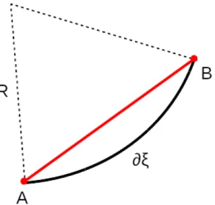
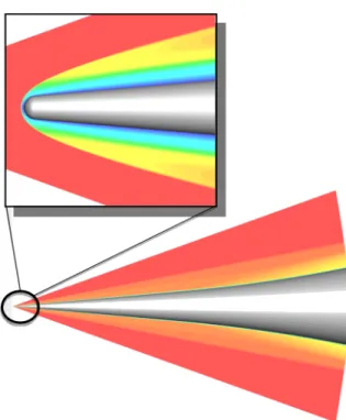
Rcis the radius of curvature measured in the streamwise marching direction for h1 and the spanwise direction for h3. A negativeRc denotes concave curvatures; positive is convex. Finally, y is the normal distance away from the surface and ∂ξ is the constant streamwise step size. The derivation for these metric terms comes from the definition of a curvilinear coordinate system. If each curve is considered in its own planar direction, the metric coefficient represents the distance traveled along the curved path (arc length) over the equivalent straight line distance. In the absence of any curvature, these lengths are equal and the ratio reduces to 1. An exaggerated visual example can be seen in figure II.1. This formulation breaks down in the limit of a straight line because Rc → ∞ and the metric coefficient must be assigned the correct value of 1.
Note thath2 does not have a curvature; this will be the wall normal grid. In the interest
of demonstrating a complete derivation for a general 3D curvilinear systemh2 will remain
in the final equations, but for our purposes h2 = 1.
II.2 Basic-State Equations
Foregoing the curvilinear terms for a moment, the dimensional governing equations for a thermally perfect gas in Cartesian coordinates are listed below.
Figure II.1: Exaggerated visualization of curvilinear transformation. Let points A and B represent two sequential points along the surface. The curved surface, black line, possesses a radius of curvatureR, which we assume remains constant over this entire step. Traveling from point A to B, the black line AB
_
represents the physical path and the red line ABrepresents the computational path. The curvature terms account for this.
ρ∗ ∂ ~u ∗ ∂t∗ +u~ ∗• ∇u~∗ ! =∇ " −P∗+µ∗ ∂u ∗ i ∂x∗j + ∂u∗j ∂x∗i ! +δijλ∗∇ ∂u∗k ∂x∗k # , i= 1,2,3 (II.2) ρ∗Cp∗DT ∗ Dt = DP∗ Dt + (∇ •κ ∗∇)T∗+µ∗ 2 ∂u∗i ∂x∗j + ∂u∗j ∂x∗i !2 +λ∗ ∇ •u~∗2 (II.3) ∂ρ∗ ∂t∗ +∇ • ρ ∗u~∗ = 0 (II.4) P∗ =ρ∗R∗gT∗ (II.5) The Navier-Stokes equations, represented as equation (II.2), apply the principles of
X-, Y-, and Z- momentum conservation of a compressible fluid. Equations (II.3)-(II.5) define energy conservation, mass continuity, and the equation of state for a thermally perfect gas, respectively. These equations are then expanded and converted to a general 3D curvilinear coordinate systems as stated in the above section. For brevity, the results will be shown after we nondimensionalize. By using these equations, we have made the following assumptions:
1. The fluid is a Newtonian fluid. 2. There is no body force.
3. There are no chemical reactions.
4. Heat transfer and thermal conductivity follows Fourier’s Law.
5. The pressure and temperature are in ranges that allow us to accurately model the gas as a thermally perfect ideal gas.
II.2.1 Thermodynamic Properties
By making the thermally perfect ideal gas assumption, listed above as assumption (5), we are forcing our compressibility factor Z = ρ∗RP∗∗
gT∗ = 1. This holds very well if the absolute pressure is near 0 atm abs or if the temperature is above the critical temperature, 133 K for air. It should be observed that at extreme temperatures this assumption will break down. Vibrational excitation begins to take place around a pressure and temperature combination of 1 atm abs and 800 K. Furthermore, oxygen begins to dissociate around 2500 K, forcing the inclusion of chemical nonequilibrium reactions. We can successfully achieve hypersonic speeds that avoid necessitating these reactions as long as care is taken when determining the freestream conditions, but there certainly exists an upper bound where our governing equations will no longer apply. The following mathematical methods used to study stability can be applied, with care, to a different set of governing equations that would account for phenomena such as thermal and chemical nonequilibrium, however we will save those derivations for future research.
For our present situation, a thermally perfect ideal gas model allows us to establish transport quantities as constants or functions of temperature (T) only. Specific heat for constant pressure (Cp), specific heat for constant volume (Cv), and ratio of specific heats (γ) will be held constant, based on an initialized reference point. Thermal conductivity (κ)
and dynamic coefficient of viscosity (µ) will be defined using Sutherland’s Law,
µ=µ0 T T0 3/2 T0+Sµ T +Sµ (II.6) κ=κ0 T T0 3/2 T0+Sκ T +Sκ (II.7) which can also be represented as
µ= C1T 3/2 T +Sµ (II.8) κ= C2T 3/2 T +Sκ (II.9) where C1 = µ0 T03/2 (T0+Sµ) = 1.458e−6 kg m·s·K1/2, Sµ= 110.40K C2 = κ0 T03/2 (T0+Sκ) = 2.49e−3 kg·m s3·K3/2, Sκ = 194.00K
are the values used for perfect air. This formulation allows for the easy inclusion of any ideal gas with Sutherland constants. Finally, thermodynamic equilibrium allows the use of Stokes’ Hypothesis to set
λ=−2
II.3 Nondimensionalization
All variables in equations (II.2)-(II.5) are nondimensionalized by their relative edge quantities, denoted by a subscript e. The edge refers to a location where perturbations have died out and only basic-state quantities remain. It is typically defined as the edge of the boundary layer, but can also be defined by freestream values, sometimes denoted as a ‘‘reference’’ quantity. Pressure is nondimensionalized by dynamic pressure, ρ∗eUe∗2, both
viscosity coefficients byµ∗e, and time by LU∗∗
e. All dimensionless quantities are shown below.
u= Uu∗∗ e v = v∗ U∗ e w= ˜ w∗ U∗ e x= x∗ L∗ y= y∗ L∗ z = z ∗ L∗ T = TT∗∗ e ρ = ρ∗ ρ∗ e µ= µ∗ µ∗ e κ = κ∗ κ∗ e Cp = C∗ p Cp∗e = 1 Cv = C ∗ v Cve∗ = 1 t= t∗UL∗∗ e P = P∗ ρ∗ eUe∗2 Rg = R∗g R∗ ge = 1 λ= λ∗ µ∗ e L ∗ ≡qµ∗ ex∗ ρ∗ eUe∗
We choose to define our length quantity, L∗, as the boundary-layer reference length. We also define the following dimensionless quantities.
Re≡ ρ ∗ eUe∗L∗ µ∗e P r≡ Cp∗µ∗e κ∗e γ ≡ Cp∗ Cv∗ M 2 ≡ Ue∗2 γR∗gTe∗
The equations below are the result of equations (II.2)-(II.5) in nondimensional 3-D curvilinear coordinates.
X-Momentum ρ ∂u ∂t + u h1 ∂u ∂x + v h2 ∂u ∂y + w h3 ∂u ∂z −v v h1h2 ∂h2 ∂x − u h1h2 ∂h1 ∂y +w u h3h1 ∂h1 ∂z − w h1h3 ∂h3 ∂x =− 1 h1 ∂P ∂x + 1 Re 1 h1 ∂ ∂x λ h1h2h3 ∂h2h3u ∂x + ∂h1h3v ∂y + ∂h1h2w ∂z + 1 Re 1 h1h2h3 ∂ ∂x 2µh2h3 1 h1 ∂u ∂x+ v h1h2 ∂h1 ∂y + w h3h1 ∂h1 ∂z + 1 Re 1 h1h2h3 ∂ ∂y µh1h3 h2 h1 ∂ ∂x v h2 +h1 h2 ∂ ∂y u h1 + 1 Re 1 h1h2h3 ∂ ∂z µh1h2 h1 h3 ∂ ∂z u h1 +h3 h1 ∂ ∂x w h3 + µ Re 1 h1h2 ∂h1 ∂y h2 h1 ∂ ∂x v h2 +h1 h2 ∂ ∂y u h1 + µ Re 1 h3h1 ∂h1 ∂z h1 h3 ∂ ∂z u h1 +h3 h1 ∂ ∂x w h3 − 2µ Re 1 h1h2 ∂h2 ∂x 1 h2 ∂v ∂y+ w h3h2 ∂h2 ∂z + u h1h2 ∂h2 ∂x − 2µ Re 1 h1h3 ∂h3 ∂x 1 h3 ∂w ∂z + u h1h3 ∂h3 ∂x + v h3h2 ∂h3 ∂y (II.11)
Y-Momentum ρ ∂v ∂t + u h1 ∂v ∂x+ v h2 ∂v ∂y + w h3 ∂v ∂z −w w h3h2 ∂h3 ∂y − v h3h2 ∂h2 ∂z +u v h1h2 ∂h2 ∂x − u h1h2 ∂h1 ∂y =− 1 h2 ∂P ∂y + 1 Re 1 h2 ∂ ∂y λ h1h2h3 ∂h2h3u ∂x + ∂h1h3v ∂y + ∂h1h2w ∂z + 1 Re 1 h1h2h3 ∂ ∂y 2µh1h3 1 h2 ∂v ∂y+ w h3h2 ∂h2 ∂z + u h1h2 ∂h2 ∂x + 1 Re 1 h1h2h3 ∂ ∂z µh1h2 h3 h2 ∂ ∂y w h3 +h2 h3 ∂ ∂z v h2 + 1 Re 1 h1h2h3 ∂ ∂x µh2h3 h2 h1 ∂ ∂x v h2 + h1 h2 ∂ ∂y u h1 + µ Re 1 h3h2 ∂h2 ∂z h3 h2 ∂ ∂y w h3 +h2 h3 ∂ ∂z v h2 + µ Re 1 h1h2 ∂h2 ∂x h2 h1 ∂ ∂x v h2 +h1 h2 ∂ ∂y u h1 − 2µ Re 1 h3h2 ∂h3 ∂y 1 h3 ∂w ∂z + u h1h3 ∂h3 ∂x + v h3h2 ∂h3 ∂y − 2µ Re 1 h1h2 ∂h1 ∂y 1 h1 ∂u ∂x+ v h1h2 ∂h1 ∂y + w h3h1 ∂h1 ∂z (II.12)
Z-Momentum ρ ∂w ∂t + u h1 ∂w ∂x + v h2 ∂w ∂y + w h3 ∂w ∂z −v v h3h2 ∂h2 ∂z − w h3h2 ∂h3 ∂y +u w h1h3 ∂h3 ∂x − u h3h1 ∂h1 ∂z =− 1 h3 ∂P ∂z + 1 Re 1 h3 ∂ ∂z λ h1h2h3 ∂h2h3u ∂x + ∂h1h3v ∂y + ∂h1h2w ∂z + 1 Re 1 h1h2h3 ∂ ∂z 2µh1h2 1 h3 ∂w ∂z + v h3h2 ∂h3 ∂y + u h1h3 ∂h3 ∂x + 1 Re 1 h1h2h3 ∂ ∂y µh1h3 h2 h3 ∂ ∂z v h2 +h3 h2 ∂ ∂y w h3 + 1 Re 1 h1h2h3 ∂ ∂x µh2h3 h3 h1 ∂ ∂x w h3 +h1 h3 ∂ ∂z u h1 + µ Re 1 h3h2 ∂h3 ∂y h2 h3 ∂ ∂z v h2 + h3 h2 ∂ ∂y w h3 + µ Re 1 h1h3 ∂h3 ∂x h3 h1 ∂ ∂x w h3 +h1 h3 ∂ ∂z u h1 − 2µ Re 1 h3h2 ∂h2 ∂z 1 h2 ∂v ∂y+ u h1h2 ∂h2 ∂x + w h3h2 ∂h2 ∂z − 2µ Re 1 h3h1 ∂h1 ∂z 1 h1 ∂u ∂x+ w h3h1 ∂h1 ∂z + v h1h2 ∂h1 ∂y (II.13)
Energy ρ ∂T ∂t + u h1 ∂T ∂x + v h2 ∂T ∂y + w h3 ∂T ∂z = (γ−1)M2 ∂P ∂t + u h1 ∂P ∂x + v h2 ∂P ∂y + w h3 ∂P ∂z + 1 P rRe 1 h1h2h3 ∂ ∂x κh2h3 h1 ∂T ∂x + ∂ ∂y κh1h3 h2 ∂T ∂y + ∂ ∂z κh1h2 h3 ∂T ∂z +(γ−1)M 2 Re " (2µ+λ) 1 h1 ∂u ∂x + v h1h2 ∂h1 ∂y + w h3h1 ∂h1 ∂z 2 +µ h3 h2 ∂ ∂y w h3 +h2 h3 ∂ ∂z v h2 2# + " (2µ+λ) 1 h2 ∂v ∂y + w h3h2 ∂h2 ∂z + u h1h2 ∂h2 ∂x 2 +µ h3 h1 ∂ ∂x w h3 +h1 h3 ∂ ∂z u h1 2# + " (2µ+λ) 1 h3 ∂w ∂z + u h1h3 ∂h3 ∂x + v h3h2 ∂h3 ∂y 2 +µ h2 h1 ∂ ∂x v h2 +h1 h2 ∂ ∂y u h1 2# +2λ 1 h1 ∂u ∂x+ v h1h2 ∂h1 ∂y + w h3h1 ∂h1 ∂z 1 h2 ∂v ∂y + w h3h2 ∂h2 ∂z + u h1h2 ∂h2 ∂x +2λ 1 h1 ∂u ∂x + v h1h2 ∂h1 ∂y + w h3h1 ∂h1 ∂z 1 h3 ∂w ∂z + u h1h3 ∂h3 ∂x + v h3h2 ∂h3 ∂y +2λ 1 h2 ∂v ∂y + w h3h2 ∂h2 ∂z + u h1h2 ∂h2 ∂x 1 h3 ∂w ∂z + u h1h3 ∂h3 ∂x + v h3h2 ∂h3 ∂y (II.14) Continuity ∂ρ ∂t + 1 h1h2h3 ∂(h2h3ρu) ∂x + ∂(h1h3ρv) ∂y + ∂(h1h2ρw) ∂z = 0 (II.15) Equation of State γM2P =ρT (II.16)
II.4 Disturbance Equations
In order to formulate the disturbance equations, a first order perturbation is superposed upon each flow variable. We let φwith no superscript represent the total instantaneous value of our flow variables (u, v, w, T,ρ, P, µ, λ, andκ), whileφand φ0 will represent the steady basic-state and unsteady disturbance quantities respectively.
φ=φ(x, y) +φ0(x, y, z, t), φ0φ (II.17) Note that the thermodynamic quantities are only a function ofT and must be related to
x,y, and z. The perturbations of these quantities will be modeled by Taylor Expansion derivatives, resulting in the following relations:
µ0 = ∂µ ∂TT 0, λ0 = ∂λ ∂TT 0, κ0= ∂κ ∂TT 0, ∂λ ∂T = λ µ ∂µ ∂T. (II.18)
Adding the steady and unsteady parts results in the total instantaneous value. By substi-tuting equations (II.17) and (II.18) into (II.11)-(II.16), the full governing equations for the instantaneous value results. The basic state by itself is still a solution to these governing equations. This allows for the subtraction of equations (II.11)-(II.16) from the instantaneous result, culminating in the isolation of the disturbance equations.
Pressure can be eliminated from the problem by using the perturbed form of equation (II.16) to give a final disturbance equation in the form
B0 ∂φ0 ∂t +B1 ∂φ0 ∂x +B2 ∂φ0 ∂y +B3 ∂φ0 ∂z +C1 ∂2φ0 ∂x2 +C2 ∂2φ0 ∂y2 +C3 ∂2φ0 ∂z2 +D1 ∂ 2φ0 ∂x∂y +D2 ∂2φ0 ∂x∂z +D3 ∂2φ0 ∂y∂z +F0φ 0 =N L (II.19)
whereφ0 = [u0, v0, w0, T0, ρ0]T and B0,B1, . . . ,F0 are 5×5 matrices containing only
column of nonlinear terms. The next objective is to solve for the disturbance quantities, φ0. These quantities must be real in order to solve the governing equations given earlier.
II.4.1 Boundary Conditions
In order to formulate a numerical solution, a set of boundary conditions must be applied.
ywall = 0,
u0 =v0=w0 =T0= 0 Constant Wall Temperature
u0 =v0=w0 = ∂T∂y0 = 0 Adiabatic Wall
y → ∞, u0 =v0 =w0 =T0 =ρ0 = 0 Subsonic ∂u0 ∂y = ∂v0 ∂y = ∂w0 ∂y = ∂T0 ∂y = ∂ρ0 ∂y = 0 Supersonic (II.20)
Equation (II.20) portrays the boundary conditions applied to the disturbance quantities throughout the various solution methods. These conditions are representative of what we expect from a disturbance in the boundary-layer. At the wall, the no-slip condition demands the total instantaneous values u=v=w= 0, thus requiring u0 =v0 =w0 = 0. The basic-state values must already independently fulfill the no-slip condition, accounting for u=v=w= 0. If given a non-adiabatic wall condition, this also applies to T(ywall). We ensure ymax is sufficiently far away from the wall (but still within the shock if one is present) so that the other half of the boundary conditions can be safely applied. This simply declares ymax as the location where the perturbations have died out. The subsonic and supersonic conditions can be interchanged, but this setup provides the conditions that we have found to give us the most clear and consistent results.
II.5 Disturbance Quantity Formulation
Thus far no assumptions about what form the disturbance quantities take have been imposed. The following sections will address three different approximations we can make in order to solve for these quantities. Chapter III will formulate numerical methods to solve
each of the three methods.
II.5.1 Linear Stability Theory
Linear stability theory (LST) will be used to generate initial conditions for the more accurate parabolized stability equations below. LST is based upon three main assumptions:
1. The basic state is ‘‘locally parallel.’’
2. Disturbances are small enough to eliminate nonlinear interactions. 3. Unsteady disturbances take the form
φ0(x, y, z, t)≡φˆ(y)ei(αx+βz−ωt)+c.c. (II.21) Assumption (1) states that there can be no flow in the basic-state wall normal direction,
v≡0, and that the other basic-state quantities are only functions ofy, such thatu=u(y),
w = w(y), T = T(y), and ρ = ρ(y). Assumption (3), a wave equation, results from applying Fourier transformations in xand z and a Laplace transformation int. The wave amplitude ( ˆφ) is complex, which necessitates the addition of the complex conjugate (c.c.) because the disturbance (φ0) must remain real. The unsteady disturbance amplitude is a function of only y, similar to the steady basic state, and the phase is a function of x, z, t.
LST can be solved as a temporal or spatial problem. Due to its role in the following solution methods, only thespatial stability problem will be addressed here. We forceω to be real and allowαandβto be complex, thus allowing our wave disturbance amplitude to grow or decay exponentially in space. αr andβr represent the nondimensional streamwise and spanwise wave number respectively (λx = 2αrπ and λz= 2βrπ) while ω is the nondimensional frequency (ω= 2f∗UπL∗ ∗
e , f
∗ is frequency in Hz). Applying the above assumptions and (II.21) to equation (II.19) results in
A∂
2φˆ ∂y2 +B
∂φˆ
whereA,B, andC are 5×5 linear matrices based on the parameters α, β, ω, φ
for each
y point at a specific x location. These matrices can be seen in full in appendix B. The remaining relations needed to solve the problem are
θk= arctan βr αr and θki= arctan βi αi ,
which define the phase angle and the disturbance growth direction respectively. Given a specifiedω,βr, and βi at our streamwise location, a solution can be found for αr and αi. Typically,βi will be defined as 0 to define the disturbance growth in the marching direction. Then the sign ofαi will determine the stability of the given frequency at the specifiedx location.
αi <0, amplified disturbances; unstable
αi = 0, no change in space; neutral
αi >0, damped disturbances; stable
II.5.2 Linear Parabolized Stability Equations
The parabolized stability equations have become a popular method for stability analysis because of their improvements over LST. The linear parabolized stability equations (LPSE) eliminate the ‘‘locally parallel’’ assumption that LST requires. In doing this, LPSE also delivers a marching solution that reflects upstream influences. In order to derive the LPSE disturbance form, we take advantage of the fact that basic-state quantities change rapidly in the surface normal direction as compared to the surface streamwise direction. This allows us to use a WKB approximation to decompose our disturbance into a rapidly varying ‘‘wave function’’ and a slowly varying ‘‘shape function.’’
φ0(x, y, z, t)≡ φˆ(˜x, y) | {z } Shape Function ei Rx˜ ˜ x0α(x)∂x+βz−ωt | {z } Wave Function +c.c. (II.23)
We relate our slow and fast scales through ˜x= Rex . Our streamwise derivatives now take the form ∂φ0 ∂x = 1 Re ∂φˆ ∂x˜ +iα ˆ φ ! ei Rx˜ ˜ x0α(x)∂x+βz−ωt +c.c. (II.24) ∂2φ0 ∂x2 = " 1 Re2 ∂2φˆ ∂x˜2 + i2α Re ∂φˆ ∂x˜ + iφˆ Re ∂α ∂x˜ −α 2φˆ # ei Rx˜ ˜ x0α(x)∂x+βz−ωt +c.c. (II.25)
We notice that there is an elliptic term in equation (II.25), but that it isO 1
Re2
. By an order of magnitude analysis, we choose to neglect the term ∂∂x2φ2ˆ, resulting in a parabolic
equation instead. As numerous papers have previously shown [4, 3, 11], this is a good approximation because most of the ellipticity is captured in the combination of theiαφˆand
∂φˆ
∂x terms. Note that the basic state is assumed to be in the ‘‘fast scale’’ so when performing the calculations we do not actually perform the ∂x∂ = Re1 ∂∂x˜ substitution.
Finally, substituting equation (II.23) into equation (II.19) and dropping the ∂x∂22 terms
results in A∂ 2φˆ ∂y2 +B ∂2φˆ ∂x∂y+C ∂φˆ ∂y +D ∂φˆ ∂x +Eφˆ= 0. (II.26)
Once again, A,B,C,D, andE are all 5×5 linear matrices and our problem statement is now parabolic. These matrices have been fully detailed in appendix C. Finding a solution will require an initial condition (LST result) along with the boundary conditions (II.20), as well as a marching scheme and normalization parameter. This and more will be discussed in our problem formulation in the following chapter.
II.5.3 Nonlinear Parabolized Stability Equations
The nonlinear parabolized stability equations (NPSE) are derived in a similar manner as LPSE, but employ a finite-amplitude disturbance instead of the infinitesimally small amplitudes assumed in the previous two methods. By eliminating this approximation, nonlinear disturbances come into play and must be accounted for. As in LPSE, the total disturbance is still assumed periodic in the temporal and spanwise directions, so again a Fourier transformation is utilized.
φ0(x, y, z, t)≡ ∞ X n=−∞ ∞ X k=−∞ A0(n,k) φˆ(n,k)(˜x, y) | {z } Shape Function ei Rx˜ ˜ x0α(n,k)(x)∂xei(kβ0z−nω0t) | {z } Wave Function (II.27)
However, for NPSE, the transformation is applied to each mode, represented by (n, k).
A0(n,k)is the initial amplitude being applied to each particular mode. Operations are applied
the same to NPSE as they were to LPSE, including the parabolization technique. Inserting (II.27) into (II.19) and performing a harmonic balance leads to a system of equations
∞ X n=−∞ ∞ X k=−∞ " A∂ 2φˆ ∂y2 +B ∂2φˆ ∂x∂y +C ∂φˆ ∂y +D ∂φˆ ∂x+E ˆ φ # (n,k) A0(n,k)e iR˜x ˜ x0α(n,k)(x)∂xei(kβ0z−nω0t) ) =N L(n,k) (II.28)
where each (n, k) mode corresponds to an individual system of equations. The left hand operators in brackets are the same as in the LPSE equation (II.26) except that each mode has its own particular α(n,k) and ˆφ(n,k). Additionally, ω and β must be replaced withnω0
and kβ0 respectively.
TheN L right-hand side contains the 5×1 array of nonlinear terms. Our harmonic balance ensures that theN L terms will be of the form
N L(n,k) =X n1 X n2 X k1 X k2 n A0(n1,k1)A0(n2,k2)N L (quad) (n,k) ei Rx x0α(n1,k1)(x)∂xei Rx x0α(n2,k2)(x)∂xei((k1+k2)β0z+(n1+n2)ω0t)o +X n1 X n2 X n3 X k1 X k2 X k3 n A0(n1,k1)A0(n2,k2)A0(n3,k3)N L (cubic) (n,k) ei Rx x0α(n1,k1)(x)∂xei Rx x0α(n2,k2)(x)∂xei Rx x0α(n3,k3)(x)∂xei((k1+k2+k3)β0z+(n1+n2+n3)ω0t)o (II.29)
wheren1,n2,. . . ,k3are all summed from−∞to∞,n1+n2(+n3) =n, andk1+k2(+k3) =k, thus giving a matching phase speed with the linear terms on the left hand side. The unique system of equations for each (n, k) mode are now coupled by the nonlinear terms. The full nonlinear matrix is expanded in appendix D.
Because the disturbances must still be real, the solution requires the use of complex conjugates ( ˆφ†). These are accounted for through symmetry properties.
α†(n,k)=−α(−n,−k) β † 0(n,k) =β0(−n,−k) A0(† n,k)=A0(−n,−k) uˆ†(n,k) = ˆu(−n,−k) ˆ v†(n,k)= ˆv(−n,−k) wˆ † (n,k) = ˆw(−n,−k) ˆ T(†n,k)= ˆT(−n,−k) ρˆ † (n,k) = ˆρ(−n,−k) (II.30)
If the basic state exhibits a z-direction symmetry, we can additionally set the following properties. The z-symmetry does not apply for modes with n= 0, as these are already
covered by (II.30). α(n,k)=α(n,−k) β0(n,k) =β0(n,−k) A0(n,k)=A0(n,−k) uˆ(n,k) = ˆu(n,−k) ˆ v(n,k)= ˆv(n,−k) wˆ(n,k) =−wˆ(n,−k) ˆ T(n,k)= ˆT(n,−k) ρˆ(n,k) = ˆρ(n,−k) (II.31)
Note that because the complex conjugate is required to formulate a real disturbance, the initial amplitude a particular mode experiences will be double (A0(n,k)+A†0(n,k)). For clarity, when applying an initial amplitude ofA0 to a mode, we actually applyA0/2 to the mode
and its complex conjugate, (n, k) and (−n,−k).
Finally, the unique mode (0,0), the mean flow distortion, will be addressed in chapter III.
III. NUMERICAL FORMULATION
This chapter focuses on formulating a numerical solution for the equations derived in the previous chapter. The solution for the linear stability problem (II.22) will follow Malik’s BVM method [31]. Solutions for both the linear and nonlinear parabolized stability equations (II.26 and II.28) will be aided by Herbert and Bertolotti’s methods [4, 11].
III.1 Computational Grid
We begin by reducing the system of second-order differential equations into a system of algebraic equations by way of finite-difference methods. In order to perform an accurate finite differentiation, the first step is to discretize our data; we create a grid with uniformx
(ξ) andy (η) to perform our stability calculations on.
Uniformxis a straightforward discretization using surface distance (Xs) of the starting and ending point along with the desired number of streamwise marching points (N x).
∂ξ= Xsend−Xs0
N x (III.1)
This gives a constant step size, which is cumulatively added toXs0 to build uniformξ. Because the stability calculations require a high resolution in the boundary layer, the uniform normal (η) grid will be treated differently. If η were formed in the same manner as ξ, achieving the accuracy required in the boundary layer would require an extremely large number of points. In order to save computation time and minimize the number of normal points (N y), a uniform normal grid (η) is created and algebraically mapped to a wall clustered computational normal grid (yc) defined by
yc= aη
b−η, (III.2)
η∈[0,1], yc∈[0, ymax] a= ymaxycrit ymax−2ycrit , b= 1 + a ymax .
This relation puts half of our normal points (N y) between yc= 0 and yc=ycrit, where
ycrit is preselected accordingly. ymax is defined as far enough away from the wall to apply the y → ∞ boundary conditions from equation (II.20). Finite differences in the normal direction can now be calculated with a constant ∆η spacing and then related to the new computational grid through
∂ ∂yc = ∂ ∂η ∂η ∂yc ∂2 ∂yc2 = ∂2 ∂η2 ∂η ∂yc 2 + ∂ ∂η ∂2η ∂yc2 (III.3)
where ∂yc∂η and ∂yc∂2η2 can be calculated directly from equation (III.2).
Note that for ease of use, transformation (III.3) may be applied by declaring our previously unused h2 term as
h2 = 1/ ∂η ∂yc, ∂h2 ∂y =−h 3 2 ∂2η ∂yc2. (III.4)
All otherh2 derivatives should remain 0, and then ∆η is used as the spacing for y-derivative finite differences. This can be seen from the following relationship:
Grid Transformation Curvilinear Derivative ∂φ ∂yc = ∂φ ∂η ∂η ∂yc 1 h2 ∂φ ∂η ∂2φ ∂yc2 = ∂2φ ∂η2 ∂η ∂yc 2 +∂φ ∂η ∂2η ∂yc2 1 h22 ∂2φ ∂η2 − 1 h32 ∂h2 ∂yc ∂φ ∂η
All of the following calculations are performed on the computational grid (ξ, yc). For simplicity only, the rest of the equations will refer to the (x, y) grid (e.g. the term ∂u∂x actually refers to ∂u∂ξ and ∆ξ should be used in finite derivatives, NOT ∆x).
III.2 Finite-Difference Method
By mapping to a uniform computational grid, we permit the use of standard finite-difference methods. Wall normal derivatives will be solved with a fourth order central finite difference scheme, ∂φˆj ∂y = −φˆj+2+ 8 ˆφj+1−8 ˆφj−1+ ˆφj−2 12∆y ∂2φˆj ∂y2 = −φˆj+2+ 16 ˆφj+1−30 ˆφj+ 16 ˆφj−1−φˆj−2 12∆y2 , (III.5)
where applicable. Boundaries will utilize second order left- or right-sided scheme and one point off from boundaries will utilize a central second order scheme.
Because the LPSE and NPSE equations are parabolized and no longer elliptical, we must used a different scheme for the streamwise derivatives. By utilizing a second order left-sided finite difference scheme,
∂φˆj
∂x =
3 ˆφj−4 ˆφj−1+ ˆφj−2
2∆x , (III.6)
our equations will be influenced by upstream values, but immune to the downstream effects. Again, accuracy must be decreased to a first order scheme when one point off of a boundary.
III.3 Local Eigenvalue Solution
In order to solve the LST equation (II.22), an eigenvalue problem approach will be used. By applying a fourth order central finite difference scheme (III.5), the problem simplifies to a system of algebraic equations with five unknowns ( ˆφj =
h ˆ
uj,ˆvj,wˆj,Tˆj,ρˆj iT
) at each y
location. Boundary conditions (II.20) are then applied to y1 and ymax. In addition we are left with an unknown global complex α that is independent of they location.
This system’s solution can be obtained by treating the complex α as an eigenvalue and the associating vector of ˆφs as the corresponding eigenvector. To account for the nonlinearity of α that occurs in the viscous terms, the following transformation is applied.
ˆ Φj = ˆ uj ˆ vj ˆ wj ˆ Tj ˆ ρj αuˆj αˆvj αwˆj αTˆj (III.7)
The eigenvalue problem now takes the form
A andB now constitute 9N y×9N ymatrices; correspondingly ˆΦ is a 9N y×1 eigenvector. Matrix Ais built by assuming α= 0, conversely matrixB will contain only the α andα2
coefficients. Some basic identity formulas relating ˆΦ values ( ˆΦj(1) =αΦjˆ (6)) round out the final equations needed in order to solve the entire system.
EPIC utilizes a QZ algorithm to solve equation (III.8), resulting in the full eigenvalue spectrum of 9N y results. Many of these will be spurious results. At this point, filters must be applied in order to pick the most unstable (most negativeαi), physical eigensolution.
The linear stability theory provides a localized stability solution that carries the as-sumptions addressed in chapter II. As mentioned earlier, one unstable location is not indicative of laminar-to-turbulent transition. LST can be performed along a path and the collected growth rates can be integrated to ascertain if and how much a disturbance grows downstream, however EPIC is designed to use the LST solution as an initial value for the more accurate PSE methods.
III.4 Linear Marching Procedure
The LPSE solution method employs a marching scheme to solve the boundary value problem (BVP) at each x location, one step at a time. Instead of creating an eigenvalue problem at each step, the previous steps’ solutions formulate an initial guess that justifies solving the BVP in an iterative fashion, reducing its computational expense. LST cannot adopt this method unless an approximate solution is already known.
A fourth order central finite difference scheme (III.5) is again applied in the normal direction. Due to the parabolic nature of the problem, a left-sided finite difference scheme (III.6) is implemented for the streamwise derivatives instead of a central scheme. This permits us to forgo involving downstream values to solve our current step while simulta-neously accounting for upstream influences. Upon applying the finite difference schemes, the resulting algebraic system is arranged to form a pentadiagonal-block matrix on the left hand side.
C1 D01 E10 A01 B20 C2 D02 A3 B3 C3 D3 E3 . .. . ..
AN y−2 BN y−2 CN y−2 DN y−2 EN y−2 BN y−0 1 CN y−1 D0N y−1 EN y0 A0N y BN y0 CN y ˆ φ1 ˆ φ2 ˆ φ3 .. . .. . ˆ φN y−2 ˆ φN y−1 ˆ φN y = RHS1 RHS2 RHS3 .. . .. . RHSN y−2 RHSN y−1 RHSN y (III.9) TheAj,Bj,Cj,Dj, andEj terms represent 5×5 matrices at that location. Each ˆφj and
RHSj are 5×1 vectors. Matrices near the boundary using the different finite differencing stencils (as mentioned previously) are denoted by 0. Furthermore, the equations denoted by blocks j= 1 and j=N y will reflect the imposed boundary conditions (II.20).
The coefficient matrices are based onφx, αx,β, andω, wherexdenotes our current step location. Additionally, the right hand side (RHS) vectors include ˆφx−1 and ˆφx−2. From a
marching standpoint, the equation (III.9) can also be expressed as
Axφˆx =Bxφˆx−1+Cxφˆx−2, (III.10)
whereAx is the 5N y×5N y pentadiagonal-block matrix and the rest of the components are 5N y×1 vectors.
As briefly mentioned earlier, the LST solution makes an appropriate initial condition to formulate the RHS in equation (III.9). If provided an αx, then the vector ˆφx can be best solved with a simple LU decomposition scheme. The result is then used to formulate an error, which is iteratively driven toward zero. In our tests, a simple Newton-Raphson method proved to be more than sufficient; it yielded accurate convergence with minimal time and computational costs. α is independent of the normal direction, thus we expect
that α will change slowly in the streamwise direction and we formulate our initial guess by assuming no change from the previous step.
∂αx
∂x =
αx−αx−1
∆x = 0 (III.11)
III.4.1 Normalization Condition
Our iterative solver still requires a solution condition in order to converge. To ensure that the shape function is slowly varying in the streamwise direction, a normalization condition is imposed upon it that will become the solution condition. A standard normalization condition has the form
Z ∞
0 ∂
∂xΨ∂y= 0 (III.12)
where Ψ is the parameter to be normalized. Because our shape function is a complex value ( ˆφr+iφˆi), both its magnitude (kφˆk) and its phase (arctan
ˆ φi ˆ φr ) must be normalized. In simplifying both of the normalization parameters,
Z ∞ 0 ∂ ∂x kφˆk∂y−−−−−−→reduces to 2 Z ∞ 0 ˆ φr ∂φˆr ∂x + ˆφi ∂φˆi ∂x ! ∂y (III.13) Z ∞ 0 ∂ ∂x arctan ˆ φi ˆ φr !! ∂y−−−−−−→reduces to Z ∞ 0 ˆ φr∂ ˆ φi ∂x −φˆi ∂φrˆ ∂x ˆ φ2 r+ ˆφ2i ! ∂y (III.14)
the driving values to be normalized can be reduced to ˆφr∂
ˆ φr ∂x + ˆφi ∂φiˆ ∂x and ˆφr ∂φiˆ ∂x −φˆi ∂φrˆ ∂x. This conveniently allows us to formulate one solution condition,
Z ∞
0
ˆ
φ†∂φˆ
∂x∂y=errr+ierri (III.15)
resulting in a complex error value. The real error will constrain the magnitude while the imaginary error constrains the phase. This error is subsequently used in the Newton-Raphson iterations to adjust the complexαaccordingly. The resulting ˆφs from solving (III.9) with newαs will eventually reduce both normalization parameters to within a predefined
tolerance. Once this tolerance is reached, the α and ˆφs for that streamwise location are saved, a step is taken in the marching direction, and the process is repeated downstream. Remember however that ˆφrepresents five distinct variables (ˆu, ˆv, ˆw, ˆT, ˆρ), whereas
α can only be refined by one single quantity. Instead of trying to select the most crucial term, we opt to combine all five terms. This will ensure that all aspects of the flow are evolving downstream as they should. Furthermore, a Pythagorean normalization parameter is applied to our solution condition so that modes comprised of very small magnitudes do not bypass the tolerance. Our final normalization parameter takes the form
Z ∞ 0 ˆ u†∂uˆ ∂x + ˆv †∂ˆv ∂x+ ˆw †∂wˆ ∂x + ˆT †∂Tˆ ∂x + ˆρ †∂ρˆ ∂x ! ∂y maxφˆ∗φˆ†
=errr+ierri. (III.16)
III.5 Nonlinear Marching Procedure
The NPSE problem is reminiscent of solving multiple, coupled LPSE problems. Each mode (n, k) has a unique equation (II.28) that is coupled through the nonlinear terms. In the interest of finding a numerical solution, analysis is restricted to −N ≤ n ≤ N and
−K ≤k≤ K. If we have a wave with frequency F and initial amplitude A, we expect that the harmonics 2F, 3F, 4F, . . . will possess initial amplitudes ofA2,A3,A4, . . . , thus eliminating the extremes is not a severe restriction. More computational costs can be saved by exercising the symmetry laws shown previously (equations II.30 and II.31) whenever possible. All modes will exhibit real physical disturbances, meaning only modes (0≤n≤N,
−K ≤k≤K) must be calculated. Furthermore, only modes (0≤n≤N, 0≤k≤K) need be solved if a geometry exhibits z-axis symmetry.
Applying the same finite difference schemes and boundary conditions as exercised in the LPSE method results in a similar pentadiagonal-block matrix system for each mode (n, k) with the addition of the relevant nonlinear terms on the right hand side. These nonlinear terms will contain unknown ˆφx terms, and so we must incorporate a nonlinear convergence loop into our marching. When guessing anαx (equation III.11), we will also make an initial
![Figure IV.3: Wall temperature distributions for the Langley 93-10 flared cone, showing the experimental conditions in the M6QT [14], the adiabatic distribution, and the computational model of 398K.](https://thumb-us.123doks.com/thumbv2/123dok_us/1875609.2773873/55.918.259.676.164.507/temperature-distributions-langley-experimental-conditions-adiabatic-distribution-computational.webp)