Sharp-Crested Weir Discharge Coefficient

(1)

J

ournal of

C

ivil

E

ngineering and

U

rbanism

Volume 3, Issue 3: 87-91 (2013) (Received: December 13, 2012; Accepted: May 7, 2013; Published: May 30, 2013) ISSN-2252-0430

Sharp-Crested Weir Discharge Coefficient

Hadi Arvanaghi

1

, Navid Nasehi Oskuei

2

1

Assistant Professor, Water Engineering Department, Faculty of Agriculture, University of Tabriz, Tabriz, Iran

2

Former M.Sc. Student, Hydraulic Structures Engineering, Faculty of Agriculture, University of Tabriz, Tabriz, Iran

*Corresponding Author’s E-mail address: [email protected]

ABSTRACT: Weirs are useful and common devices in flow measurements. The essential parameter of each weir is to determine the flow coefficient. In this study, laboratory measurements of the water surface profile, approach flow velocity and flow rate carried out over three different rectangular sharp-crested weirs mounted in a flume. The flow was then numerically simulated by the CFD commercial software Fluent v. 6.2 in several stages. Results show that Fluent can model the flow over this type of weirs preciously. Then the effect of three dimensionless parameters of weir height (H/W), Froude number and Reynolds number on weir discharge coefficient is investigated using experimental and numerical data. For a specific value of these parameters, discharge coefficient is tending to the fixed value of 0.7.

Keywords: Sharp-Crested Weir, CFD, Discharge Coefficient, Weir Height, Froude Number, Reynolds Number

INTRODUCTION

Weirs have been widely used for the flow measurement, flow diversion and its control in the open channels (Kumar et al., 2011). Weirs are categorized in two main types: sharp-crested and broad-crested. Sharp-crested weirs normally consist of a vertical plate mounted at right angles to the flow and having a sharp-edged crest, as shown in Figure 1. (Henderson, 1966).

In Figure 1 W is weir height, H is water static

head and V0 is approach flow velocity.

The simplest form of these weirs consists of a plate set perpendicular to the flow in a rectangular channel, its horizontal upper edge running the full width of the channel. This last feature means that the flow is essentially two-dimensional, without lateral contraction effects. Also, so called contracted weirs exists which are contracted from the sides as well as in the vertical plane. This last type will involve three-dimensional flow (Henderson, 1966). Weirs have various shapes such as rectangular, triangular, trapezoidal, circular etc. and especial applications and governing equations. The Typical form of the governing equation of these weirs is as following (Bos, 1989):

n

Q



kH

(1)

where Q = flow rate, k = coefficient depending on the size and shape of the weir and n = dimensionless number depending on the shape of the weir. For rectangular and triangular weirs n equals to 1.5 and 2.5, respectively.

Discharge equation for a rectangular sharp-crested weir of the same width of the channel can be simplified as (Henderson, 1966): 1.5

2

3

d

Q



C

g LH

(2)

where L = crest length of the weir, Cd = discharge

coefficient, g = acceleration due to gravity and H = static head over the crest.

The Cd depends on flow characteristics and

geometry of the channel and weir (Kumar et al., 2011).

For simplicity we can consider that Cd is just dependents

on the ration H/W, for example we can use so called Rehbock equation for H/W <= 5 (Henderson, 1966):

0.611 0.08

d

H

C

W





(3)

Nowadays, we can simulate turbulent flow using advanced numerical methods. These methods are useful to determine velocity distribution, water surface profile, flow rate and some other coefficients. Computational Fluid Dynamics (CFD) commercial software such as Fluent and Flow 3D are applicable and strength tools to evaluate mentioned parameters.

Sarker and Rhodes (1999) first carried out laboratory measurements of free surface profile over a rectangular broad-crested weir. Then they numerically simulated the free surface flow by the Fluent in several stages. They also applied standard k-ε turbulence model to solve Novier-Stocks equations. They results have good conformity in comparison with experimental data. Liu et al. (2002) simulated water surface profile on semicircular weirs using k-ε turbulence model. Haun et al. (2011) calculated water flow over a trapezoidal broad-crested weir by two different CFD codes of Flow 3D and SSIM 2, where first one uses Volume of Fluid (VOF) method with a fixed grid, while last one uses an algorithm based on the continuity equation and the Marker-and-Cell method. They compared the results with measurements from a physical model study using different discharges and they state that the deviation between the computed and measured upstream water level was between 1.0 and 3.5 %. Kumar et al. (2011)

(2)

investigated the capacity of the triangular and rectangular sharp-crested weirs and they stated that the efficiency of triangular weirs is better than the rectangular one and also high for low vertex angle. They also examined the sensitivity of the weir i.e., change of discharge due to unit change in head which indicates that the weir is more sensitive at the low head and low vertex angle.

In this paper, we examined the effect of the height, Froude number and Reynolds number on discharge coefficient of rectangular sharp-crested weir. Tests are carried out both experimentally and numerically. This study is aimed to specify a range for mentioned parameters in which the weir discharge coefficient is constant.

Figure 1. Scheme of a sharp-crested weir.

MATERIALS AND METHODS

Experiments have been done in a laboratory flume with glass made walls. The flume length, width and height are 10, 0.25 and 0.5 m, respectively. Water enters the flume through a stilling system. Then flow passes over the weir and finally flow discharges to the settling basin of the flume. There is a V-notch weir downstream the settling basin which is calibrated to measure the flow rate. Water surface elevation in the flume is measured by a needle type levelmeter which accuracy is about 0.1 mm. Sharp-crested weirs of the same width of the flume (L = b = 0.25 m) are made from PVC plates in three different heights of 10, 15 and 20 cm. The weirs are mounted 6 m downstream the flume entrance (see Figure 2). Tests are iterated for each weir at least 10 times. Discharge measurements have been done after that the water head is balanced. Each weir is tested with different heads from 1 cm up to the flume height.

Figure 2 – The position and dimensions of weir in the flume.

In this study, numerical modelling is carried out by Fluent v. 6.2. Fluent is one of the powerful and common CFD commercial software. It first transforms the governing equations to the algebraic equations by finite volume method then solves them. Fluent has the ability to solve 2D and 3D problems of open channel flow, confined conduit flow and sediment transport by advanced turbulence models. Also it is possible to solve continuum and momentum equations so called Novier-Stocks equations around sharp-crested weirs.

So, reliable CFD codes such as Fluent could be successfully used to pre-optimize the aforementioned issues, saving a lot of money, time and effort. It is relatively easy to modify the geometry in a numerical model; changes in physical models are usually hard and costly to be implemented. Naturally, the CFD codes have to be efficient and accurate, and it has to be able not only to deal successfully whit the instabilities of the non-linear equations of motion, but also to compute satisfactorily the turbulence properties and to find the free surface location.

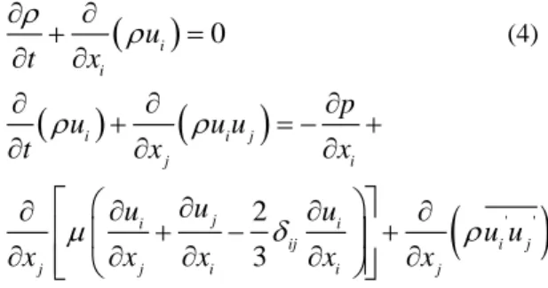
The governing equations of our interest are unsteady incompressible 2-dimensional continuity and Reynolds-averaged Novier-Stockes equations (RANS) for liquid and air (Liu et al., 2002).

 

_i

0

i

u

t

x



_









(4)

 







' '



2

3

i i j j i j i i ij i j j j i i j

p

u

u u

t

x

u

u u

x













 









































(5)

where, ρ = fluid density, u = velocity components, x = space dimensions, t = time, p = hydrostatic pressure, µ = dynamic viscosity,

u u

_i' _j'= Reynolds stress tensor and δij = crooner delta.

There are different methods to solve RANS. In this study, k-ε RNG turbulence model is used which is defined as (Papageorgakis and Assanis, 1999):

 



i



i k eff k b M k j j

k

ku

t

x

k

G

Y

S

x



 































(6)

 









2 1 3 2 i eff i j j k b

u

t

x

C

G

C G

C

R

S

k

     





 

































₍₇₎

where k = kinetic energy, ε = energy dissipation rate, Gk = turbulence kinetic energy generation due to

mean velocity gradient, Gb = kinetic energy due to

floatation, YM = turbulence Mach number and the other

parameters are model coefficients.

To start Fluent we first need to specify channel geometry and then generate a mesh for it. Gambit software is used to do this. Because three different

(3)

heights are defined for experimental models of weirs, we need to design an especial geometry and mesh for each weir (e.g. see Figure 3). In this study, more than 40 2D configurations are generated by gambit.

Figure 3 - Generated mesh by Gambit.

RESUTLS AND DISCUSSION

First, tests are carried out experimentally on three different sharp-crested rectangular weirs of the same width of the flume width. Then all configurations are simulated by Gambit and finally are modelled by Fluent. In Table 1 results of experimental and numerical investigations are represented. Using this data water surface profile over the weir and the effect of the dimensionless weir height, Froude number and Reynolds number on discharge coefficient is inquired.

Water surface profile

During each test, the water depth upstream and downstream the weir is measured after that the flow balanced. Then the water surface profile is drawn and is compared with Fluent results. Figure 4 depicts the water surface profile for one of the configurations which has

run in the Fluent. Error! Reference source not found.

is also a comparison between numerical and experimental profile. The results show the good conformity of numerical result by experimental ones.

Figure 4 - Water surface profile modeled by Fluent.

Figure 5 – Comparison of experimental and numerical water surface profile.

Dimensionless weir height

Figure 6 to Figure 8 represent dimensionless height of weir effect on discharge coefficient. As seen, for H/W > 0.4 the numerical results are very close to experimental ones and by increasing weir height this point is reached before H/W = 0.4. Figure 9 shows that after a specific value of H/W (0.6) the discharge coefficient approximately has the fixed value of 0.7 for different weir heights.

Figure 6 - Comparison of numerical and experimental Cd for different H/W (W=10 cm).

(4)

Table 1 – Results of experimental and CFD tests. No. W (cm) H (cm) y = W+H H/W q (EXP) (lit/s) V (m/s) Re Fr q (CFD) (lit/s) Cd (EXP) Cd (CFD) 1 10.00 1.00 11.00 0.10 2.97 0.03 1579.79 0.03 3.66 1.01 1.24 2 10.00 2.00 12.00 0.20 7.26 0.06 3704.08 0.06 9.15 0.87 1.10 3 10.00 3.00 13.00 0.30 13.35 0.10 6544.12 0.09 15.80 0.87 1.03 4 10.00 4.00 14.00 0.40 20.11 0.14 9485.85 0.12 20.72 0.85 0.88 5 10.00 5.00 15.00 0.50 26.61 0.18 12095.45 0.15 26.83 0.81 0.81 6 10.00 6.00 16.00 0.60 33.86 0.21 14850.88 0.17 33.77 0.78 0.78 7 10.00 7.00 17.00 0.70 40.65 0.24 17224.58 0.19 40.74 0.74 0.75 8 10.00 8.00 18.00 0.80 48.66 0.27 19942.62 0.20 48.48 0.73 0.73 9 10.00 9.00 19.00 0.90 56.49 0.30 22416.67 0.22 56.55 0.71 0.71 10 10.00 10.00 20.00 1.00 66.10 0.33 25423.08 0.24 65.85 0.71 0.71 11 10.00 11.00 21.00 1.10 74.36 0.35 27746.27 0.25 74.26 0.69 0.69 12 10.00 12.00 22.00 1.20 84.66 0.38 30673.91 0.26 84.62 0.69 0.69 13 10.00 13.00 23.00 1.30 95.45 0.42 33609.15 0.28 95.39 0.69 0.69 14 10.00 14.00 24.00 1.40 106.66 0.44 36527.40 0.29 106.60 0.69 0.69 15 10.00 15.00 25.00 1.50 118.37 0.47 39456.67 0.30 118.27 0.69 0.69 16 15.00 1.50 16.50 0.10 5.59 0.03 2409.48 0.03 6.43 1.03 1.19 17 15.00 3.00 18.00 0.20 14.22 0.08 5827.87 0.06 14.65 0.93 0.96 18 15.00 4.50 19.50 0.30 24.57 0.13 9597.66 0.09 24.72 0.87 0.88 19 15.00 6.00 21.00 0.40 33.13 0.16 12361.94 0.11 33.36 0.76 0.77 20 15.00 7.50 22.50 0.50 44.25 0.20 15803.57 0.13 44.41 0.73 0.73 21 15.00 9.00 24.00 0.60 56.15 0.23 19229.45 0.15 56.05 0.70 0.70 22 15.00 10.50 25.50 0.70 70.30 0.28 23125.00 0.17 70.39 0.70 0.70 23 15.00 12.00 27.00 0.80 85.85 0.32 27167.72 0.20 85.77 0.70 0.70 24 15.00 13.50 28.50 0.90 102.50 0.36 31250.00 0.22 102.35 0.70 0.70 25 15.00 15.00 30.00 1.00 119.86 0.40 35252.94 0.23 120.06 0.70 0.70 26 15.00 16.50 31.50 1.10 138.24 0.44 39272.73 0.25 138.36 0.70 0.70 27 15.00 18.00 33.00 1.20 156.11 0.47 42887.36 0.26 156.25 0.69 0.69 28 20.00 2.00 22.00 0.10 8.87 0.04 3213.77 0.03 9.82 1.06 1.18 29 20.00 4.00 24.00 0.20 21.98 0.09 7527.40 0.06 21.93 0.93 0.93 30 20.00 6.00 26.00 0.30 37.91 0.15 12308.44 0.09 37.91 0.87 0.87 31 20.00 8.00 28.00 0.40 51.81 0.19 15990.74 0.11 51.76 0.78 0.78 32 20.00 10.00 30.00 0.50 68.70 0.23 20205.88 0.13 68.88 0.74 0.74 33 20.00 12.00 32.00 0.60 87.80 0.27 24662.92 0.15 87.85 0.72 0.72 34 20.00 14.00 34.00 0.70 108.00 0.32 29032.26 0.17 108.21 0.70 0.70 35 20.00 16.00 36.00 0.80 129.80 0.36 33453.61 0.19 129.73 0.69 0.69 36 20.00 18.00 38.00 0.90 153.50 0.40 37995.05 0.21 153.42 0.68 0.68 37 20.00 20.00 40.00 1.00 179.45 0.45 42726.19 0.23 179.51 0.68 0.68 38 20.00 22.00 42.00 1.10 208.51 0.50 47823.39 0.24 208.65 0.69 0.69

(5)

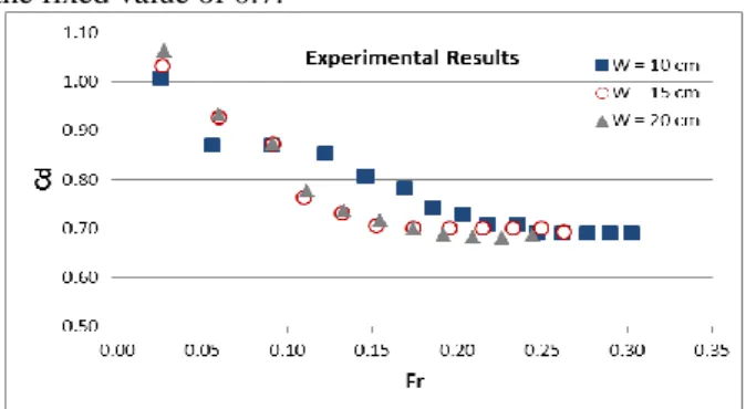
The effect of froude number on discharge coefficient

The discharge coefficient variation with Froude number for different weir heights is shown in Figure 10. The discharge coefficient for Fr > 0.2 is approximately the fixed value of 0.7.

Figure 10 - Experimental Cd vs. Fr.

The effect of reynolds number on discharge coefficient

Figure 11 represents Cd variation with Reynolds number for different values of weir heights. As seen, for Re > 20000 Cd has the fixed value of 0.7

Figure 11 - Experimental Cd vs. Re.

CONCLUSION

Rectangular sharp-crested weir is one of the flow measuring tools which are usually used in irrigation and drainage channels. The most essential parameter of discharge equation of this type of weirs is the discharge coefficient. In this study discharge coefficient of the

rectangular sharp-crested weir is investigated

experimentally and numerically. The results show that the Cd has the fixed value of 0.7 when the following condition is maintained:

H/W > 0.6 , Fr > 0.2 , Re > 20000 Beyond these boundaries, Cd is not constant and it is not recommended to use a unique Cd for different flow conditions.

Furthermore in this study the water surface profile and discharge coefficient is modelled using Fluent and is compared with experimental results. A good conformity is yielded between numerical and experimental results.

REFERENCES

1. Bos MG. (1989). Discharge measurement structures.

Third revised edition. International institute for land reclamation and improvement, 121-151.

2. Haun S, Reidar NBO, Feurich R. (2011). Numerical

modeling of flow over trapezoidal broad-crested weir. Engineering Applications of Computational Fluid Mechanics, 5(3): 397-405.

3. Henderson FM. (1964). Open-channel flow,

Macmillan, New York, 269-277.

4. Kumar S, Ahmad Z, Mansoor T. (2011). A new

approach to improve the discharging capacity of sharp-crested triangular plan form weirs. Flow Measurement and Instrumentation, 22(2011): 175-180.

5. Liu C, Hute A, Wenju MA. (2002). Numerical and

experimental investigation of flow over a

semicircular weir. Acta Mechanica Sinica, 18: 594-602.

6. Papageorgakis GC, Assanis DN. (1999).

Comparison of linear and nonlinear RNG-based models for incompressible turbulent flows. Journal of Numerical Heat Transfer, University of

Michigan, 35: 1-22.

7. Sarker MA, Rhodes DG. (1999). 3D free surface

model of laboratory channel with rectangular

broad-crested weir. Proceeding 28th IAHR Congress, Graz,