Procedia Computer Science 93 ( 2016 ) 495 – 502
1877-0509 © 2016 The Authors. Published by Elsevier B.V. This is an open access article under the CC BY-NC-ND license (http://creativecommons.org/licenses/by-nc-nd/4.0/).
Peer-review under responsibility of the Organizing Committee of ICACC 2016 doi: 10.1016/j.procs.2016.07.239
ScienceDirect
6th International Conference On Advances In Computing & Communications, ICACC 2016, 6-8
September 2016, Cochin, India
1 Trend Filter for Image Denoising
Sreelekshmy Selvin*, S.G.Ajay*, B.Ganga Gowri, V.Sowmya, K.P.SomanCentre for Computational Engineering and Networking Amrita School of Engineering, Coimbatore
Amrita Vishwa Vidyapeetham, Amrita University, India
Abstract
The major problem in digital image processing is the presence of unwanted frequencies(noise). In this paper1 trend filter is pro-posed as an image denoising technique.1-trend filter estimates the hidden trend in the data by formulating a convex optimization problem based on1 norm. The proposed method extends the application of1 trend filter from one dimensional signals to three di-mensional color images. Here the filter is applied over the image in a cascade, initially filtering along the rows followed by filtering along the columns. This identifies the hidden image information from the noisy image resulting in a smooth or denoised image. The proposed method is compared with the wavelet denoising technique using the quality metrics Peak-Signal-to-Noise-Ratio(PSNR) and Structural Similarity Index(SSIM).
c
2016 The Authors. Published by Elsevier B.V.
Peer-review under responsibility of the Organizing Committee of ICACC 2016. Keywords: Noise;Denoising; Norm;1 trend filter; Wavelet denoising; PSNR; SSIM.
1. Introduction
An image can be considered as a matrix of pixel intensity levels. The presence of abnormal variations in bright-ness or other image information is considered as a noise10. These variations cause problems in image processing
applications, real time processing and also in research. Therein lies the power of image denoising technique4. The
denoising algorithms in9can be used as a single task or as a part of other image processing algorithms. The algorithms
are classified based on their processing type into spatial domain and frequency domain methods15. Spatial domain
methods are considered to be direct and fast17. It is further classified into non-liner filters. Linear filters make use of
a statistical approach in which separate filters are used for each of the frequency response14. The main disadvantage
of the linear filters is that a prior knowledge about the spatial properties of the image and the type of noises that may
∗Corresponding author. Tel.:+91-9495149772 ;fax:+0-000-000-0000
E-mail address:[email protected]
© 2016 The Authors. Published by Elsevier B.V. This is an open access article under the CC BY-NC-ND license (http://creativecommons.org/licenses/by-nc-nd/4.0/).
affect the image is needed. Also if there is a change in the frequency response of the system, the filter should also be modified accordingly. Nonlinear filters use windowing or masking operations for denoising. A window is ann×n
matrix which replaces each of the pixel intensity levels with its median value. This method is robust as the median of the data is taken instead of the mean value of the image. But, as the size of the image increases this method fails and the process becomes more complex and time consuming. Transform domain filtering mainly include data transform techniques7such as Wavelet Transform1 8, Fast Fourier Transform11, Discrete Wavelet Transform1and so on. It is
classified into two categories adaptive and non-adaptive data transform methods. Data adaptive transforms makes use of the underlying hidden information for denoising. Independent Component Analysis is an important method that falls under the category of data adaptive denoising algorithms13. The drawback of this method2is that it requires a
minimum of two image frames for performing denoising, which is not always possible. Also it uses a sliding window technique which makes the cost of implementation more. Non-data adaptive method considers local properties of data and such algorithms5generates an approximate representation of the data. Some of the important techniques in
this category are Wavelet transform and Fast Fourier Transform.16Wavelet-based implementation requires algorithms
which are memory intensive in nature. The basic principle of this method is the convolution of the input with standard filter coefficient14. As the input length increases, execution of the algorithm also increases. The greatest challenge
in image denoising is the preservation of image information while removing the noise. The choice of denoising al-gorithm varies depending upon the type of noise. Also, the performance of the alal-gorithm varies with the noise levels and other control parameters. In this paper, we are extending the idea of1 trend filter for one dimensional signals proposed in9to color images. The method was implemented over standard images for different noise types at varying noise levels. The quality of the denoised image was analyzed using the quality metrics:PSNR and SSIM. In section[2] we discuss the mathematical background of the proposed system. Section[3] discusses the proposed method and its subsection 3.1 discusses implementation steps. Section[4] discusses the experimental results and analysis and the comparision between wavelet denoising3and1 trend filter.
2. Mathematical Background
Norm is defined as the total size or length of all vectors in a vector space. For every single real number, a corre-sponding norm is present. Thepnorm12of a vectorxis defined as
||x||p= p
i
|xi|p (1)
i.e,pnorm is thepthroot of summation of all the elements in the vector to powerp. The mathematical properties of
pnorm varies and hence their application also varies12. The1 norm is the sum of absolute values and is not smooth.
The proposed method uses the idea of1 norm along with convex optimization. It is a variation of Hodrick-Prescott filter, where the sum of squares in HP-filter is replaced by1 norm. The1 trend filter is defined as
1
2 y−x
2
2+kAx1 (2)
The problem statement can be physically interpreted as follows. xis the original input image.yis the noisy image,k
is the control parameter andAis the second order difference of the estimated trend, The matrixAhelps in smoothing the denoised image which is given by
A=
1−2 1 1 −2 1
... ... ...
1 −2 1
The control parameterkis calculated based on the following equation
kmax=(AAT)−1Ay∞ (3)
A scalar time series may have both slowly varying component and also a rapidly varying component. The slowly varying component can be represented asxtand rapidly varying component can be represented aszt. The1 trend
filter is a convex optimization problem with the objective of getting a smooth slowly varying component and estimating the random component or residual. The residual estimation is equivalent to estimating the slowly varying component and hence it is known as filtering. The1 trend filter gives smooth trend estimates and the variations in the slope of the estimated trend can be considered as an abrupt change. The1 trend filter problem statement is given as
1 2 n t=1 (yt−xt)2+k n−1 t=2 |xt−1−2xt+xt+1| (4)
eqn.(4) is same as eqn.(2) whereAis the second order differential matrix. The optimization problem of eqn.(2) is defined as
min1
2y−x
2
2+kz1,S ub ject to z=Ax (5)
The trend estimated value minimizes the weighted sum.kis the regularization parameter which varies between (0,∞]. As (k→ ∞) it converges to the best affine fit for a finite value ofk. The value ofkis calculated as
kmax=(AAT)−1Ay∞ (6)
As (k→ 0), it will converge to original data which is given by
y−x∞≤4k (7)
The objective function eqn.(1) is convex but cannot be differentiated. To minimizex, we obtain the following condi-tion. Consider a vectorvRn, we have
y−x=ATv (8) now we have, vt ⎧⎪⎪ ⎪⎨ ⎪⎪⎪⎩ +k, (Ax)t>0 −k, (Ax)t<0 [−k,k],(Ax)t=0 ⎫⎪⎪ ⎪⎬ ⎪⎪⎪⎭
wheret=1,2....n−2. Let us consider theAmatrix in the following example
A1= 1−2 1 0 0 1 −2 1 Size ofA1is 2×4. A2= ⎡ ⎢⎢⎢⎢⎢ ⎢⎢⎢⎣10 1−2 1 0 0−2 1 0 0 0 1 −2 1 ⎤ ⎥⎥⎥⎥⎥ ⎥⎥⎥⎦
Size ofA2is 3×5. i.e., in general the size ofAmatrix is (n−2)×n. AT is of sizen×(n−2). Rank ofAis (n−2)
and that ofAATis also (n−2). SinceAATis a full rank matrix, it is invertible. From eqn.(6) we have
(y−x) = ATV (9)
pre-multiplying withAwe get
A(y−x) = AATV (∵AATis invertible) (10)
at any time we have
(AATA(y−x))t∈ ⎡ ⎢⎢⎢⎢⎢ ⎢⎢⎢⎣+−kk,, ((AxAx))tt<>00 [−k,+k],(Ax)t=0 ⎤ ⎥⎥⎥⎥⎥ ⎥⎥⎥⎦ (11)
Now eqn.(8) will become −4k≤ATV t≤4k f or any vR n−2 (12) ⇒ −4k≤xt−yt≤4k where t=1,2....n (13)
As (k → ∞), x → xbais the best affine fit for which the value ofkconverges to a finite value. Sincexbais affine, Axba=0
⇒(AAT)−1A(y−xba)
∞ = (AAT)−1Ay∞ ≤k (14)
in matrix form we have, (AAT)−1A y yn+1 − xn 2xn−xn−1 ∞ ≤k (15) whereAR(n−1)×(n+1)and (xlt,2xlt
n−xltn−1) gives the trend estimate for (y,yn+1).
3. Proposed Method
The proposed system uses1 trend filter as a image denoising technique. 1 trend filter was initially developed for one dimensional signals in9. In this paper we are extending the idea for color images in9. The proposed method
for image denoising is more efficient when compared with the wavelet denoising method. The performance of the system is validated using the metrics (PSNR) and (SSIM). The mapping of the method from one dimension to two dimensions was achieved by extracting each of the rows and columns separately and processing it.
3.1. Implementation Steps
• The input image is distorted by the addition of noise.
• The red, green and blue planes of the image is extracted separately into three different matrices.
• For each plane extracted in the previous step the following operation is performed. – Extract each row of the matrix and transpose it.
– Apply1 trend filter.
– Stack the result to a new matrix.
– Extract each column of the new matrix obtained in the previous step. – Apply1 trend filter.
– Stack the result in a different matrix which gives the denoised plane.
• Reconstruct the denoised image by combining the denoised matrices of the three planes.
Input Image Add Noise R,G,B planesExtract
Perform row wise1 trend filtering
Perform column wise1 trend filtering for the result obtained Combine the
three planes Denoised
image
4. Experimental Results and Analysis
The experiment was conducted on the standard set of images Peppers, Lena, House and Barbara of varying sizes 256×256, 512×512, 1024×1024. As mentioned above, each image was tested against different noises such as Salt and Pepper, Gaussian and Speckle at different noise levels. Gaussian noise was added to the image with zero mean and variance values such as 0.025, 0.05, 0.075, 0.1. Salt and Pepper and Speckle noise was added to the images with different mean values such as 0.025, 0.05, 0.075, 0.1. The quality of the output image was evaluated using quality metrics such as PSNR and SSIM and the results are given in Table 1. The value of control parameterkis fixed as 0.001 because lambda value below 0.001 affects the denoising and above 0.025 leads to loss of image information. The experiment is repeated for same test images and noise levels using wavelet denoising method. The results obtained using wavelet denoising method6were tabulated in Table 2. By comparing the PSNR and SSIM values in Table 1
and Table2, we can infer that the proposed method improves the PSNR and SSIM values by reducing noise in the enhanced image.
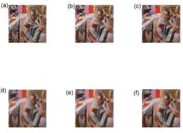
Following Fig.2,Fig.3,Fig.4 and Fig.5 shows the comparison of the noisy images with the enhanced image. From these figures, we can conclude that the propose method gives a smooth denoised image with the noises removed. Based on the noise types, the denoising of Gaussian noise gives a much smoother image comparitively.
Table 1: PSNR of noisy images (NI PSNR) and denoised images (DI PSNR) and also SSIM values for noisy images (NI SSIM) and denoised images (DI SSIM) for various noises applied to standard test images.
IMAGE NOISE TYPE NOISE LEVEL NI PSNR (dB) DI PSNR (dB) NI SSIM DI SSIM Peppers
Salt & Pepper 0.1 15.0663 22.0659 0.6448 0.888
Gaussian 0.025 19.9046 24.2103 0.8431 0.942
Speckle 0.1 16.5695 24.044 0.7328 0.9331
Lena
Salt & Pepper 0.1 15.184 24.0986 0.5821 0.9297
Gaussian 0.025 19.9787 24.1168 0.803 0.9377
Speckle 0.1 16.0396 23.8901 0.6287 0.9257
House
Salt & Pepper 0.1 15.2715 23.6765 0.4247 0.8403
Gaussian 0.025 19.9329 25.0583 0.6713 0.8993
Speckle 0.1 15.4116 24.0678 0.432 0.8555
Barbara
Salt & Pepper 0.1 15.2749 22.5541 0.385 0.7325
Gaussian 0.025 19.8397 22.5289 0.6005 0.7469
Table 2: Comparison of denoised image PSNR (DI PSNR) and SSIM (DI SSIM) values obtained from (a) Wavelet denoising technique and (b)1 trendfilter method
IMAGE NOISE TYPE NOISE LEVEL DI PSNR(dB) DI SSIM(dB)
(a) (b) (a) (b)
Peppers
Salt & Pepper 0.1 18.8937 22.0659 0.8004 0.888 Gaussian 0.025 23.4981 24.2103 0.9294 0.942
Speckle 0.1 23.2693 24.044 0.919 0.9331
Lena
Salt & Pepper 0.1 19.3831 24.0986 0.7698 0.9297 Gaussian 0.025 26.2151 24.1168 0.9529 0.9377
Speckle 0.1 24.5948 23.8901 0.9159 0.9257
House
Salt & Pepper 0.1 19.1534 23.6765 0.6175 0.8403 Gaussian 0.025 25.4796 25.0583 0.8994 0.8993
Speckle 0.1 23.8597 24.0678 0.8394 0.8555
Barbara
Salt & Pepper 0.1 20.2108 22.5541 0.5755 0.7325 Gaussian 0.025 24.4673 22.5289 0.7868 0.7469
Speckle 0.1 24.2477 22.9746 0.7559 0.7463
Fig. 2: (a) Input image with Salt and Pepper noise level 0.1 (b) Input image with Gaussian noise level 0.025 (c) Input image with Speckle noise level 0.1. (d), (e), (f) are the Output denoised images
Fig. 3: (a) Input image with Salt and Pepper noise level 0.1 (b) Input image with Gaussian noise level 0.025 (c) Input image with Speckle noise level 0.1. (d), (e), (f) are the Output denoised images
Fig. 4: (a) Input image with Salt and Pepper noise level 0.1 (b) Input image with Gaussian noise level 0.025 (c) Input image with Speckle noise level 0.1. (d), (e), (f) are the Output denoised images
Fig. 5: (a) Input image with Salt and Pepper noise level 0.1 (b) Input image with Gaussian noise level 0.025 (c) Input image with Speckle noise level 0.1. (d), (e), (f) are the Output denoised images
5. Conclusion
The paper proposes a new image denoising technique based on 1 trend filter method. The proposed method is applied on standard test images with noises of different types and levels. R,G,B planes of noisy colour images are extracted and1 trend filter method is applied on that to get denoised images. The work is an extension of
one dimensional signal denoising based on1 trend filter (proposed to two dimensional colour images in10). The
performance of the new approach is validated. From the PSNR and SSIM values obtained, it is evident that the new algorithm performs in an efficient way and gives better results than existing denoising methods.
References
1. Marc Antonini, Michel Barlaud, Pierre Mathieu, and Ingrid Daubechies. Image coding using wavelet transform.Image Processing, IEEE Transactions on, 1(2):205–220, 1992.
2. Ron Bracewell. The fourier transform and its applications.New York, 5, 1965.
3. Antoni Buades, Bartomeu Coll, and Jean Michel Morel. On image denoising methods.CMLA Preprint, 5, 2004.
4. Antoni Buades, Bartomeu Coll, and Jean-Michel Morel. A review of image denoising algorithms, with a new one.Multiscale Modeling&
Simulation, 4(2):490–530, 2005.
5. S Grace Chang, Bin Yu, and Martin Vetterli. Adaptive wavelet thresholding for image denoising and compression.Image Processing, IEEE Transactions on, 9(9):1532–1546, 2000.
6. S Grace Chang, Bin Yu, and Martin Vetterli. Adaptive wavelet thresholding for image denoising and compression.Image Processing, IEEE Transactions on, 9(9):1532–1546, 2000.
7. Ritendra Datta, Dhiraj Joshi, Jia Li, and James Z Wang. Image retrieval: Ideas, influences, and trends of the new age. ACM Computing Surveys (CSUR), 40(2):5, 2008.
8. B Ganga Gowri, V Hariharan, S Thara, V Sowmya, S Sachin Kumar, and KP Soman. 2d image data approximation using savitzky golay fil-ter ˚Usmoothing and differencing. InAutomation, Computing, Communication, Control and Compressed Sensing (iMac4s), 2013 International Multi-Conference on, pages 365–371. IEEE, 2013.
9. Vikas Gupta. A review on image denoising techniques 1. 2013.
10. Seung-Jean Kim, Kwangmoo Koh, Stephen Boyd, and Dimitry Gorinevsky. l1 trend filtering.SIAM review, 51(2):339–360, 2009. 11. Jae S Lim. Two-dimensional signal and image processing.Englewood Cliffs, NJ, Prentice Hall, 1990, 710 p., 1, 1990.
12. Ivan Markovsky and Sabine Van Huffel. Overview of total least-squares methods.Signal processing, 87(10):2283–2302, 2007.
13. Mukesh C Motwani, Mukesh C Gadiya, Rakhi C Motwani, and Frederick C Harris. Survey of image denoising techniques. InProceedings of GSPX, pages 27–30, 2004.
14. KP Soman et al.Insight into wavelets: from theory to practice. PHI Learning Pvt. Ltd., 2010.
15. KP Soman and R Ramanathan. Digital signal and image processing-the sparse way.Isa Publication, 2012.
16. M Suchithra, P Sukanya, Pinchu Prabha, OK Sikha, V Sowmya, and KP Soman. An experimental study on application of orthogonal matching pursuit algorithm for image denoising. InAutomation, Computing, Communication, Control and Compressed Sensing (iMac4s), 2013 International Multi-Conference on, pages 729–736. IEEE, 2013.
17. Mr Rohit Verma and Dr Jahid Ali. A comparative study of various types of image noise and efficient noise removal techniques.International journal of advanced research in computer science and software engineering, 3(10):617–622, 2013.