Revisiting Mutual Fund Performance Evaluation

Munich Personal RePEc Archive

Revisiting Mutual Fund Performance

Evaluation

Angelidis, Timotheos and Giamouridis, Daniel and

Tessaromatis, Nikolaos

Department of Economics University of Peloponnese

2 February 2012

Online at

https://mpra.ub.uni-muenchen.de/36644/

Revisiting Mutual Fund Performance Evaluation

Timotheos Angelidis

, Daniel Giamouridis

, Nikolaos Tessaromatis

Current version: February 2012 (First draft: August 2011)

Abstract

Mutual fund manager excess performance should be measured relative to their self-reported benchmark rather than

the return of a passive portfolio with the same risk characteristics. Ignoring the self-reported benchmark introduces

biases in the measurement of stock selection and timing components of excess performance. We revisit baseline

empirical evidence in mutual fund performance evaluation utilizing stock selection and timing measures that address

these biases. We introduce a new factor exposure based approach for measuring the – static and dynamic – timing

capabilities of mutual fund managers. We overall conclude that current studies are likely to be overstating lack of

skill because they ignore the managers’ self-reported benchmark in the performance evaluation process.

Keywords: Mutual funds, short-term performance, market timing, factor timing

JEL Classification: G11, G12, G14, G23

*

We are appreciative for the comments and suggestions of Wayne Ferson, Joop Huij, Nickolaos Travlos, Russ

Wermers and seminar participants at Boston College and at the Campus for Finance Research Conference 2012.

Daniel Giamouridis greatly acknowledges the financial support of the Athens University of Economics and Business

Research Center (ΕΡ-1681-01). Any remaining errors are our own.

1

Timotheos Angelidis is a Lecturer in Finance, Department of Economics, University of Peloponnese E-mail

address: [email protected]

2

Daniel Giamouridis is an Assistant Professor of Finance, Department of Accounting and Finance, Athens

University of Economics and Business, Athens, Greece. He is also Senior Visiting Fellow at Cass Business School,

City University, London, UK, and, Research Associate at EDHEC-Risk Institute, EDHEC Business School, Nice,

France. E-mail address: [email protected]

3

Nikolaos Tessaromatis is an Associate Professor of Finance, ALBA Graduate Business School, Athens, Greece

Revisiting Mutual Fund Performance Evaluation

Abstract

Mutual fund manager excess performance should be measured relative to their self-reported benchmark rather than

the return of a passive portfolio with the same risk characteristics. Ignoring the self-reported benchmark introduces

biases in the measurement of stock selection and timing components of excess performance. We revisit baseline

empirical evidence in mutual fund performance evaluation utilizing stock selection and timing measures that address

these biases. We introduce a new factor exposure based approach for measuring the – static and dynamic – timing

capabilities of mutual fund managers. We overall conclude that current studies are likely to be overstating lack of

skill because they ignore the managers’ self-reported benchmark in the performance evaluation process.

Keywords: Mutual funds, short-term performance, market timing, factor timing

1.

Introduction

An impressive range of researchers have investigated whether mutual fund managers are ‘able’

investors.1 Overall, this literature suggests that skill, if it exists, is evident in a small – but not

negligible – fraction of the cross-section of mutual fund managers. Critical to the study of

managerial ability is the measurement of excess performance. The current literature generally

follows either of two approaches to measure excess performance. In studies that are based on

return data, the abnormal return (the fund’s ‘alpha’) is calculated as the return of the fund in

excess of the return of a passive portfolio with the same risk characteristics. A positive alpha is

considered as evidence of managerial skill. In studies that are based on mutual fund portfolio

holdings typically the return adjustment involves controls for risks determined by the market

(beta), size, book-to-market, and momentum characteristics of the stocks held by the mutual fund

manager. Both approaches measure excess performance as if fund managers make ex-ante

investment decisions against an ex-post benchmark.

We argue in this paper that this assumption is incorrect and incosnsistent with the practice

followed by the fund management industry. Mutual fund managers are in practice evaluated

against the benchmark stated in the fund’s prospectus and their actions are to a large extent

1

Examples of stock selection studies include: Grinblatt and Titman (1992), Elton et al. (1993), Hendricks et al.

(1993), Goetzmann and Ibbotson (1994), Brown and Goetzmann (1995), Grinblatt et al. (1995), Carhart (1997),

Blake and Timmerman (1998), Bollen and Busse (2005), Kosowski et al. (2006), Barras et al. (2010), Fama and

French (2010). Examples of market, or broadly speaking factor, timing studies include: Treynor and Mazuy (1966),

Henriksson and Merton (1981), Henriksson (1984), Bollen and Busse (2001), Comer (2005), Jiang et al. (2007),

Swinkels and Tjong-A-Tjoe (2007), Mamaysky et al. (2008), Busse and Tong (2008), Elton et al. (2011),

Kacperczyk, et al. (2011). Excellent reviews of this literature are provided by Ferson (2010), Aragon and Ferson

dictated by the nature of that benchmark. Examples of frequently used benchmarks include the

S&P 500 for large stocks, the S&P 500 Value for funds with a value orientation or the S&P 500

Growth index for growth funds. The benchmarks may themselves have significant alphas as well

as significant exposures to systematic risk factors. Hence, calculating mutual fund alphas without

accounting for the fund benchmark’s alpha may bias stock selection related inferences. Similar

issues may arise in the analysis of managers’ market timing ability. Ignoring the manager’s

self-reported benchmark would incorrectly classify as timing changes in factor exposures which

merely reflect the manager’s effort to track the time-varying sensitivities of her benchmark.

To address these issues, we propose that the self-designated benchmark is directly incorporated in

the evaluation process. The importance of incorporating the fund’s self-designated benchmark in

the process of measuring mutual fund performance is stressed in other current studies too (see,

e.g. Cremers and Petajisto, 2009, Sensoy, 2009, Hsu et al., 2010, Cremers, et al., 2010). In

partcular we propose that a mutual fund’s performance is measured relative to its benchmark

performance, and any deviation be interpreted as an effort to improve the relative performance of

the managed portfolio. We show that this framework generates alphas and exposures to

systematic risks that by construction differ from those obtained through the typical approaches.

We use a standard risk model (Carhart’s 1997 model) to derive these differences. The

implications are similar if alternative models are used.

Using the proposed methodology, we revisit baseline empirical evidence in mutual fund

performance evaluation. The stock selection and timing measures we utilize are exactly parallel

to each other. We measure stock selection as the difference between the alpha of the fund and the

alpha of its self-designated benchmark. We measure timing as the differential return earned by

benchmark. Our timing measure builds on the thesis that portfolio managers implement timing

decisions through changes of the sensitivity of their portfolio to a set of aggregate factors that

affect returns (Elton et al., 2011). In this context, we further argue that a manager may seek to

exploit long term risk premia (beta, size, value, or momentum) by taking long-term positions that

are different relative to the average exposure of her benchmark (static factor allocation). Also she

may take short-term tactical bets when she believes that current market conditions favor a

particular investment style (dynamic market allocation).

In the first part of our empirical analysis, we study the impact of incorporating the fund’s

self-designated benchmark into the performance evaluation process for stock selection releted

inferences. We find in our sample, consistent with the current empirical evidence, that mutual

fund alphas are on average negative. However, alphas estimated with the approach we advocate

are generally less negative and less statistically significant than the alphas computed with the

typical approach in the literature. This finding reflects the fact that the commonly used

self-designated benchmarks have negative alphas in the sample period. The differences between the

approach we advocate and the standard approach are more pronounced when we focus on mutual

funds of particular investment styles. The average alpha for example of small cap growth funds is

-4.02% (t-statistic=-2.54) per annum when it is computed with the standard approach. Using our

approach the average alpha rises to -2.04 per annum and becomes statistically insignificant

(t-statistic=-1.08). Ignoring the self-designated benchmarks in our sample generally puts growth

mutual funds managers as a group at a disadvantage vis a vis value fund managers.

Next, we study the implications of the proposed framework for measuring timing. We find

convincing empirical evidence of significant timing by mutual fund managers. More than half

timing decisions. More than a third of all managers take statistically significant bets against the

factor exposures of the self-designated benchmarks. Despite the importance of timing decisions,

timing makes a small contribution to total mutual fund performance. Our evidence suggests that

on average mutual funds underperform their benchmarks by 2% per annum. Almost three

quarters of that underperformance is due to bad stock selection decisions. The negative

contribution of stock selection is significant and consistent across all investment styles. Timing,

and in particular dynamic factor timing, contributes -0.5% per annum to average mutual fund

underperformance. Elton et al. (2011) also report negative albeit larger in absolute terms, timing

returns. Not accounting for the fund’s benchmark may misclassify – with respect to their timing

skill – funds that simply track the sensitivities of their benchmark to systematic risk factors.

This article makes several contributions to the existing literature. First, we study mutual fund

performance within a context that is more in line with current institutional asset management

practices. We find that ignoring the fund’s benchmark leads to biased assessments of a

manager’s performance. Second, we introduce a new factor exposure based approach for

measuring the timing capabilities of mutual fund managers that utilizes mutual fund return data.

From a conceptual point of view, our approach is consistent with the notion that managers – on

top of stock selection – move assets in and out of various sectors and securities as part of a

dynamic factor timing strategy. Our apporach has advantages over existing approaches that rely

on mutual fund holdings data. Moreover, our approach on factor timing skill measurement

disentangles the two aspects of factor timing that is, short- and long-term. Thirdly, we provide

new empirical evidence on the importance of stock selection versus timing decisions.

Our findings add new insights to the literature on mutual fund performance evaluation. The use

evaluation practices, overstates the finding of lack of managerial skill. The ‘explicit’ benchmark

plays a central role in portfolio construction and risk management in current investment

management practices. Pure stock selection decisions account for less than 50% of portfolio

tracking error. A significant portion of active risk is due to factor timing decisions and in

particular factors like value, size and momentum. This has implications for manager evaluation,

manager selection, risk budgeting and risk management practices of institutional investors.

This paper proceeds as follows. In Section 2 we discuss the inconsistency (with asset

management practice) of the risk-adjustment approach that most studies have in common and

demonstrate what amendments we believe are necessary to maintain consistency. We also

develop a new method for measuring factor timing skill. Section 3 discusses the data we use in

our empirical analysis. Section 4 illustrates the impact of inappropriate risk-adjustment on

measuring stock selection skill. It also reports the results of the analysis on the factor timing

ability of mutual fund managers which uses the proposed method. Section 5 presents the results

of the robustness analysis and Section 6 concludes.

2.

Measuring Skill against a Self-designated Benchmark

2.1 Self-designated versus Implicit Benchmark

The standard approach for measuring skill in the literature uses the following regression:

, , 1( , , ) 2 3 4 ,

i t f t i i m t f t i t i t i t i t

R −R = +a β R −R +β SMB +β HML +β MOM +e (1)

where R_{i t,} is the return of fund i, R_{f t,} is the short term risk free rate at time t, R_{m t,} is the return

market value, book-to-market, and past returns (Carhart, 1997) all at time t; e_{i t,} is he residual

return of fund i at time t. For ease of exposition we remove the time subscript hereafter.

This framework implicitly assumes that the appropriate benchmark for the evaluation of a

particular portfolio is implicit in the returns generated by the manager’s portfolio. To estimate the

implicit benchmark typically equation (1) is estimated and the implicit benchmark return, denoted

as ˆ

b

implicit

R , is calculated through:

1 2 3 4

ˆ ˆ ˆ ˆ

ˆ _{( )}

b

implicit

i m f i i i

R =β R −R +β SMB+β HML+β MOM (2)

The fund’s alpha is then taken to be the difference between the fund’s average return and the

average return of the implicit benchmark, that is:

(

)

ˆ

b

implicit i i f

a = R −R −R (3)

In practice however mutual fund managers are evaluated against the self-designated benchmark

stated in the fund’s prospectus rather than the estimated implicit benchmark.2 Their active

decisions – stock selection and factor timing – are taken with reference to the self-designated

benchmark. Risk management and reporting also uses the self-desgnated benchmark.

To the extent that the self-designated benchmark and the implicit benchmark are similar, in terms

of performance and factor exposures, estimates from equation (1) will adequately measure the

contribution of active decisions to mutual fund performance. For this to happen, the

self-designated benchmark should exhibit zero alpha and should have the same exposures to the risk

2

Becker et al. (1999) in fact provide evidence that mutual funds behave as benchmark investors. Sensoy (2009) also

stress that consistent with agency theory investors (principals) influence fund companies’ (agents) compensation –

factors as the implicit benchmark. However, recent studies (see, e.g. Cremers, et al., 2010)

suggest that commonly used benchmarks, such as those used by mutual fund managers as

self-designated benchmarks, have non-zero alphas. For example using the following regression:

1( ) 2 3 4

b f b b m f b b b b

R −R =a +β R −R +β SMB+β HML+β MOM +e (4)

where R_b is the return of a benchmark, may result in sample estimates of a_b that are not

necessarily zero. In fact, when we conduct preliminary analysis in our sample we find significant

variation in the estimates of ab,β β βb₁, b₂, b₃, and βb₄ ranging from negative to positive.

3

This

practically means that alphas and betas estimated through equation (1) are biased measures of

skill. The size of bias depends on the alphas and the betas of the respective benchmarks.

Therfore we propose to measure managerial ability using the following regression:

* * * * * *

1( ) 2 3 4

i b i i m f i i i i

R −R =a +β R −R +β SMB+β HML+β MOM+e (5)

where R_b is the return of fund i’s self-designated benchmark. Provided that managers are

evaluated with respect to their benchmark, it is more appropriate to focus on the alpha and risk

components of the return of the fund in excess of its benchmark return, to judge the manager’s

ability. The estimated exposures in equation (5) represent the difference between the fund’s and

the self-designated benchmark average exposures to the systematic factors assumed to drive

returns. We use a standard risk model (Carhart’s 1997 model) to derive these differences. The

implications are similar if alternative risk models are used.

3

To illustrate what * * * * *

1 2 3 4

, , , ,

i i i i i

a β β β β measure in equation (5), we substract equation (4) from

equation (1) and get:

(

) (

)

(

)

(

)

(

)

(

)

(

)

1 1 2 2 3 3

4 4

i b i b i b m f i b i b

i b i b

R R a a R R SMB HML

MOM e e

β β β β β β

β β − = − + − − − − + − + − + + (6)

Therefore from (5) and (6) we infer that:

* *

or

i i b i i b

a =a −a a =a +a (7)

* *

1 1 1 or 1 1 1

i i b i i b

β =β −β β =β +β (8)

* *

2 2 2 or 2 2 2

i i b i i b

β =β −β β =β +β (9)

* *

3 3 3 or 3 3 3

i i b i i b

β =β −β β =β +β (10)

* *

4 4 4 or 4 4 4

i i b i i b

β =β −β β =β +β (11)

Equations (7) to (11) show that the estimates of a fund’s alpha and factor exposures obtained

through equation (1) include the benchmark’s exposures to factor returns. That is, the alpha

estimated from equation (5) is equal to the alpha estimated from equation (1) using the standard

methodology of performance evaluation less the alpha of the benchmark. We argue that *

i

a is a

more relevant estimate for manager’s ability compared to the usual a_i estimate. *

i

a measures the

manager’s ability to add value through stock selection relative to the benchmark. In contrast a_i

includes in addition to stock selection skill the abnormal return inherent in the benchmark which

by definition cannot be influenced by the manager’s actions. Equation (8) also suggests that the

market beta estimated from equation (5) is equal to the market beta estimated from equation (1)

a portfolio with beta different to the beta of the benchmark. For example an estimated excess

market beta of -0.2 means that the fund’s beta is 0.2 smaller than the beta of the benchmark.

Similar interpretations hold for the value, size, and momentum exposures.

2.2 Timing as Excess Factor Exposure

The previous section develops a framework that we argue is more appropriate for measuring

mutual fund managers’ excess performance. In this section we introduce a new framework for

assessing a manager’s timing ability. Our timing measure builds on the thesis that portfolio

managers implement timing decisions through changes of the sensitivity of their portfolio to a set

of aggregate factors that affect returns (Elton et al., 2011).

We use high frequency (daily) data, over a short time interval, i.e. one month, to estimate a

mutual fund’s factor exposures through equation (5).4 We measure factor timing returns as the

product of exposure at time t times the average factor return over time t, as follows:

n * * * *

1 2 3 4

ˆ ˆ ˆ ˆ

timing skill_i =β_i (R_m −R_f)_t+β_i SMBt+β_i HMLt+β_i MOMt (12)

Since we estimate equation equation (5) using daily data over a monthly horizon, for each month

we get estimates for * * * *

1, 2, 3, 4

i i i i

β β β β . Hence, in equation (12), timing skilln_i is our estimate of

average timing skill for fund i for month t, and (R_m−R_f) ,_t SMB HMLt, t, and MOMt are average

daily premiums observed over month t.

4 _{The choice of a monthly horizon is justified on several grounds. First it addresses to some extent the impact of style}

breaks in mutual fund style exposures documented by Annaert and Campenhout (2007). Second, it is consistent with

the evidence in Mamaysky et al. (2008) who find that many U.S. mutual funds follow highly dynamic strategies at

the monthly frequency. Third, it leaves enough data to compute statistically sound estimates while at the same time

This measure is very closely related to the measures utilized by Elton et al. (2011), Jiang et al.

(2007), and Kacperczyk, et al. (2011). These studies make use of mutual fund portfolio holdings

and estimates of individual stock factor exposures to calculate portfolio exposures. Timing is

then assessed on the basis of the portfolio exposure at time t and the return of the factor at time

t+1. Each measure has some advantages. We use return data which makes our approach less

sensitive to the availability of mutual fund holding data at high frequencies. Elton et al. (2010)

stress that the use of quarterly data misses 18.5% of a typical fund’s trades revealed using

monthly data. Monthly holdings data however are not broadly available. The sample in Elton et

al. (2010) comprises (after cleaning) 215 funds in the period 1994-2005. In addition, we define

our timing measure by means of the contemporaneous factor return. This choice allows us to

capture potential changes in the fund portfolios as well as variations in the fund benchmark

sensitivity to the systematic risk factors over the month that performance is measured. More

importantly however, our measure explicitly accounts for the funds self-designated benchmark.

Thus, we can use it to detect the actions of the fund manager that relate to timing rather than

actions that relate to tracking the benchmark. In this respect our measure also closely relates to

the Active Share measure utilized in Cremers and Petajisto (2009) that uses mutual fund

holdings.

To get additional insight in the timing ability of managers we pursue a decomposition of the

manager’s timing ability into short- and long-term in the spirit of Hsu et al. (2010). We argue

that a manager may seek to exploit long term relationships that have shown to prevail in certain

stock market segments, while she may also dynamically adjust the factor loadings in her portfolio

al. (2010) term these two timing practices static factor allocation and dynamic market allocation

respectively and utilize holdings data for their calculations.

We propose measuring short- and long-term timing using equation (12). Equation (12) can be

re-written in terms of the long-term average excess factor exposures and long-term average factor

premiums and current factor deviations from the average as follows:

n

(

)

(

)

(

)

(

)

* * *

1 1 1

* * *

2 2 2

* * *

3 3 3

* * *

4 4 4

ˆ ˆ ˆ

timing skill ( ) ( )

ˆ ˆ ˆ

( ) ( )

ˆ ˆ ˆ

( ) ( )

ˆ ˆ ˆ

( ) ( )

i i m f i m f

i

i i i

i i i

i i i

R R R R

SMB SMB

HML HML

MOM MOM

β β β

β β β

β β β

β β β

= − − + − + − + + − + + − + dynamic static (13)

where β β βˆi*₁, ˆi*₂, ˆi*₃, and βˆi*₄ are long term average excess exposures. Equation (13) suggests that

timing skill for each factor is the sum of two components. The first component is defined as the

monthly deviation of excess factor exposure from average excess exposure, times the

contemporaneous factor return. The deviation reflects short term tactical decisions to over- or

under-weight a particular investment style in response to economic and market conditions. For

example the manager could overweight small capitalization stocks if she thinks that they are

likely to outperform large capitalization stocks in the current market environment. In equation

(13) this will be infered through the term

(

)

β

β

is defined as the product of long term average excess exposure times the average factor premium.

It measures the return contribution of a manager’s decision to tilt her portfolio persistently

hopes to benefit from the well-documented value premium. In equation (13) this is captured with

the term *

3

ˆ (_i HML)

β , through

β

(2011) who measure timing by means of variation of holdings-based betas with respect to a target

beta. Their target beta is defined as the average beta for the mutual fund portfolio over the entire

period.

3.

Data

We source mutual fund daily return data from the CRSP Mutual Fund database from September

1998 to January 2009. Risk factor and style portfolio returns are obtained from Kenneth French's

website.5 The research questions we posit require that the fund’s self-designated benchmark is

known. We focus on active equity mutual funds that fall in the intersection of value/growth and

large/small cap strategies. CRSP provides information about the investment objective of each

fund (Lipper objective code) which enables us to infer each fund’s self-designated benchmark.

Lipper’s objective codes are assigned based on the language that the fund uses in its prospectus to

describe how it intends to invest. For example, “Large-Cap Core Funds” are described as funds

that, by portfolio practice, invest at least 75% of their equity assets in companies with market

capitalizations (on a three-year weighted basis) greater than 300% of the dollar-weighted median

market capitalization of the middle 1,000 securities of the S&P SuperComposite 1500 Index.

Large-cap core funds have more latitude in the companies in which they invest. These funds

typically have an average price-to-earnings ratio, price-to-book ratio, and three-year

sales-per-share growth value, compared to the S&P 500 Index”. From this description we infer that the

5

benchmark for “Large-Cap Core Funds” is the S&P 500 Index.6 Daily benchmark returns are

obtained from Datastream.

The equity mutual funds we thus consider include nine categories: Cap Core Funds,

Large-Cap Growth Funds, Large-Large-Cap Value Funds, Mid-Large-Cap Core Funds, Mid-Large-Cap Growth Funds,

Mid-Cap Value Funds, and Small-Cap Core Funds, Small-Cap Growth Funds, and Small-Cap

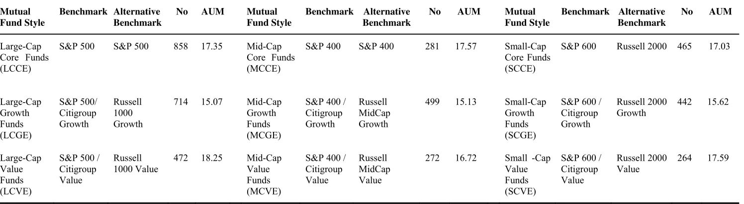
Value Funds. Table 1 tabulates the categories of funds for which we source data from CRSP for

our analysis, their inferred benchmark, alternative benchmarks, as well as the number of funds

that fall in each category in our entire sample. Large cap funds outnumber the midcap and small

cap funds by a factor of about two that is, the total number of funds is 2,044 for large cap funds

versus 1,052 and 1,171 for midcap and small cap respectively. There are 1,655 growth funds,

1,604 core funds, and 1,008 value funds. Large cap value funds are those managing on average

the largest portfolios in terms of assets with about $18.25 million NAV. Large cap growth funds

have the lowest average NAV that is $15.07 million.

[Table 1 about here]

4.

Empirical Results

This section reports and discusses the results from our empirical analysis. The first sub-section

presents estimates of a manager’s alpha based on the conventional risk adjustment methodology

and compares them with the alphas obtained with our proposed approach. The second

sub-section reports evidence on the time variance of mutual fund factor betas and investigates the

6

contribution of the varying betas in mutual fund returns. In the last sub-section we study the

stock selection and factor timing decisions’ contribution to mutual fund tracking error risk.

4.1 Mutual Fund alphas

Average returns based on daily data are computed for each month for the entire cross-section of

funds in each group in the intersection of value/growth and large/small cap strategies, and are

subsequently averaged over the entire sample period. Average returns are computed also for all

value to growth funds unconditional on size as well as for large to small cap funds unconditional

on value/growth, as well as for our pooled sample.

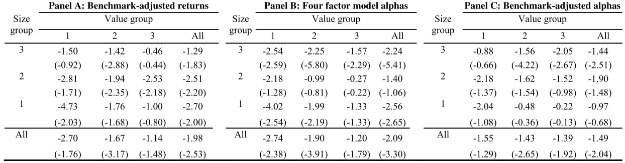
Panel A of Table 2 reports the average mutual fund return in excess of the return of the

self-designated benchmark without any risk adjustment. The evidence suggests that on average

mutual fund managers underperform their self-designated benchmarks. The average annualized

underperformance of all funds for the period of study is 1.98% (t-statistic = -2.53). The

underperformance is consistent and statistically significant across all size groups. The

underperformance is significant for growth and core managers but insignificant for value

managers.

Panel B of Table 2 tabultaes the results from the analysis with the standard model, i.e. equation

(1). We obtain negative alphas across all size and value/growth investment styles. For all funds,

the average annualized alpha is 2.09% (t-statistic=-3.30). Bollen and Busse (2005), who also use

daily data but a different sample period, find an average alpha of -1.20% per annum (Table 1, p.

577). Average alpha is consistently negative and statistically significant across the value/growth

investment styles. Large and small cap mutual fund managers also underperform significantly on

a risk adjusted basis. Managers of mid-cap funds have negative but statistically insignificant

obtained when we use the raw, i.e. not risk-adjusted, difference between fund and self-designated

benchmark returns (Panel A). However, the former leads generally to more statistically sound

conclusions regarding average alpha.

[Table 2about here]

Panel C of Table 2 presents alphas estimated from equation (5), that is from the model that

directly incorporates the self-designated benchmark in the performance evaluation process. The

average alpha we find for all mutual fund investment styles is -1.49% per annum and it is

significantly different from zero (t-statistic = -2.04). The average alpha is by 0.6% smaller than

the alpha produced by the to-date standard model in Panel B. The difference reflects the negative

alpha implicit in the self-designated benchmarks and is suggestive of the bias introduced when

the benchmarks is not taken into account when computing risk-adjusted performance. The

magnitude of the estimated average alphas using the methodology we advocate are generally

speaking lower and less statistically significant that the alphas based on the standard model. The

differences among the two methodologies are more pronounced when we examine the different

investment styles seperately.

Growth mutual funds produce on average alpha of -2.74% (t-statistic=-2.38) when the

conventional methodology is used to adjust for risk, compared with an average alpha of -1.55%

(t-statistic=-1.29) when we use our approach to measure alpha. Similarly large capitalization

mutual funds, in Panel B, produce an average alpha of -2.24% (t-statistic=-5.41). We document a

significantly lower underperformance with our approach (average alpha is -1.44% with a

t-statistic of -2.51). The differences in alpha reflect by construction the presence of negative

alphas in the self-designated benchmarks. The differences in estimated alphas are even bigger for

cap growth mutual funds is -2.54% compared with the average alpha of -0.88% which is

computed with our approach. The -1.66% difference in estimates is equal to the alpha of the S&P

500/Citigroup Growth index when the four factor model is used to adjust for risk. The difference

in estimated alphas is even more pronounced for small cap growth funds (-4.02% versus -2.04%)

or small cap core funds (-1.99% versus -0.48%). The conventional risk adjustment methodology

produces more negative alphas for growth funds than other investment style groups. When all

funds are ranked by their alphas, growth fund managers as a group will rank lower than value or

core managers with the standard approach.

Collectively, the results in Table 2 highlight the importance of taking the self-designated

benchmarks into account when measuring excess mutual fund performance. When we pool all

funds, we conclude that the average mutual fund manager is in fact destroying value by

generating negative excess returns after fees that are statistically different from zero (as in, e.g.

Jensen, 1968, Elton et al., 1993, Carhart, 1997 and Fama and French, 2010). However, alphas

estimated using our approach are generally less negative and less statistically significant than the

alphas produced by the to-date standard methodology. Our analysis indicates that for some

investment styles the differences in inferences are more pronounced and more economically

significant than in others. Overall, we conclude that the current literature is likely to be

overstating the lack of stock selection skill of mutual fund managers simply because it ignores the

managers’ bencmarks in the measurement of excess performance.

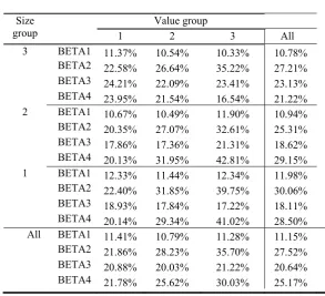
4.2 Static versus Dynamic Factor Timing in Mutual Fund Performance

In this section we report evidence on the time variance of mutual fund factor betas and

investigate the contribution of the varying betas in mutual fund returns. We measure mutual fund

Every month we estimate equation (5) using daily data and maintain excess risk exposures

relative to the self-designated benchmark’s risk exposures, for the entire cross-section of funds in

each group and in the intersection of value/growth and large/small cap strategies. For each fund

we compute statistics that capture the time variance properties of the estimates of the beta

coefficients across the entire sample period. These statistics are then averaged across funds in the

cross-section of funds in each group in the intersection of value/growth and large/small cap

strategies. Average statistics are computed also for all value to growth funds unconditional on

size as well as for large to small cap funds unconditional on value/growth, and for the entire

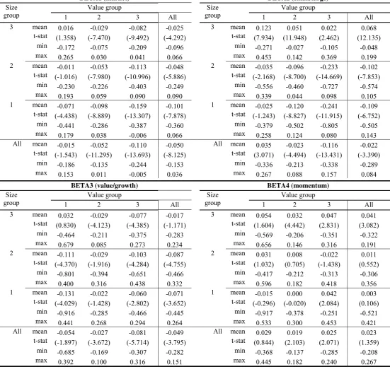
sample. In particular we report the average, minimum, and maximum deviation of each fund’s

exposure to the market portfolio (BETA1), the capitalization factor (BETA2), the value-growth

factor (BETA3), and the momentum factor (BETA4) from the respective benchmark exposures as

defined in equation (5). We also report the t-statistic for the null hypothesis that the average

deviation is zero. In unreported analysis (available on request) we find that the deviation of each

fund’s exposure from the respective benchmark’s exposure is statistically different from zero for

up to about 43% of the times it was estimated.

[Table 3 about here]

Examining Table 3 in detail provides useful insights. All investment styles, with the exception of

large growth funds, take on average less market risk than the respective benchmarks. The

t-statistics suggest a strong rejection of the hypothesis that fund managers hold portfolios with the

same market risk as that of the benchmark. Table 3 illustrates that value mutual fund managers

hold portfolios with less market risk (lower market betas) than their benchmarks. In contrast

managers of growth mutual funds have the same market risk as their benchmarks. Small cap

Large cap managers tend to tilt their portfolios more towards small cap and momentum stocks

than their benchmarks imply. The difference in exposures gets larger as we move from growth to

value portfolios. Funds with small cap investment styles in contrast, tend to have less exposure

to the small cap factor. Value and growth style managers tend to take less exposure to value

stocks than the exposure inherent in their self-designated benchmarks. Value and funds that

invest in large cap stock tend to invest more heavily in momentum stocks.

Overall, the results in Table 3 document that the average manager largely engages in timing

practices. The average deviations from the benchmark market, size and value/growth betas are

-0.050 (t-statistic = -8.12), -0.022 (t-statistic = -3.39), and -0.049 (t-statistic = -3.80) respectively.

The average deviation from the benchmarks momentum exposure is not significantly different

from zero. In general factor exposure differences increase as we move from large to small cap

and from growth to value investment styles. The evidence is consistent with the hypothesis that

managers dynamically adjust portfolio factor exposures, presumably reflecting their views about

the future performance of the systematic factors that drive stock returns.

[Table 4about here]

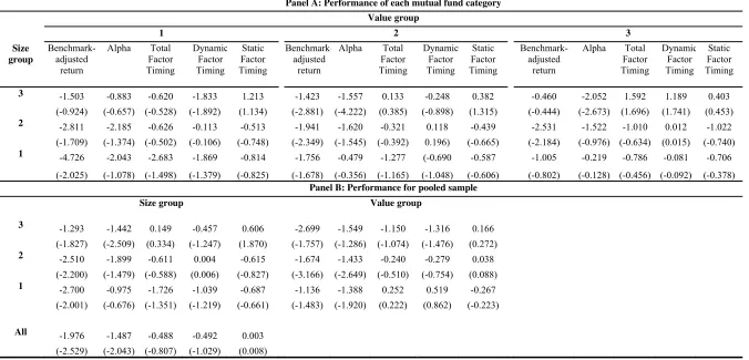
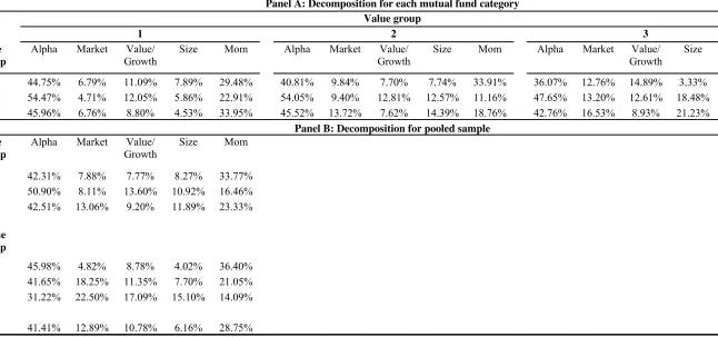
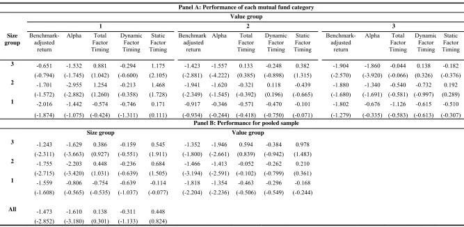
Our second objective is to study the economic implications of managers decsions to vary their

betas. In Table 4 Panel A, for each mutual fund category, we decompose the average mutual fund

benchmark adjusted return, that is the average R_i−R_b, into its components: the average

annualized alpha return estimated through equation equation (5), and the average annualized total

factor timing return computed through equation (12). We also decompose the total factor timing

return into the short-term and long-term timing returns for each group of funds that fall in the

aggregate average annualized benchmark-adjusted return, alpha return, total factor timing return,

and short- and long-term timing return for the different size and value groups.

The results reported in Panel A (Table 4) suggest that the average return differences are negative

and statistically significant for the small growth, mid and large core, and mid value investment

styles. The underperformance is mainly due to bad stock selection skills, especially for large cap

fund managers where the return differences are statistically significant. Neither static nor

dynamic timing decisions make a statistically significant contribution to mutual fund

performance.

The return decomposition for all funds is shown in Panel B of Table 4. Mutual fund managers

underperform their self-designated benchmarks by about 2% per annum (t-statistic=-2.53). Three

quarters of that underperformance is due to the negative contribution of stock selection decisions

and the remaining due to bad timing skills. The contribution of timing decisions is not

statistically different from zero. The 0.5% per annum underperformance due to timing decisions

is mainly due to return generated from the dynamic timing decisions. Elton et al. (2011) report a

more negative timing return (-0.11% per month). Hence we stress that not accounting for the

fund’s benchmark may misclassify – with respect to their timing skill – funds that simply track

the sensitivities of their benchmark to systematic risk factors.

The overall conclusion from the results presented in Table 4 is that the underperformance of the

average mutual fund is mainly due to unsuccessful stock selection decisions. Timing, and in

particular dynamic factor timing, makes a negative but statistically insignificant contribution to

mutual fund performance. The contribution of negative timing returns is less significant than the

4.3 What is important? Stock selection or, factor timing?

In the earlier analysis we concluded that the contribution of stock selection decisions is on

average negative. We also found that managers engage in factor timing, without however being,

on average, successful in this practice. In this section we examine how each component

contributes to the total variation of mutual fund excess returns.

To study this issue we decompose the variance of excess returns into an alpha and a factor timing

return component. The contribution of alpha variance is calculated as the ratio of the variance of

realized mutual fund alpha to the variance of total benchmark adjusted fund returns. The

contribution of factor timing variance is calculated as the variance of the return due to timing bets

on the market, size, value/growth and momentum factors (see equation (12)). Table 5reports the

percentage of the total variance that is attributed to the variance of each individual component.

Overall, it appears that the variance of alpha contributes about 40% of the total variance of the

mutual fund excess return. The second most important contributor is the variance of momentum

(28.75%). Market and value/growth rank almost equally with 12.89% and 10.78% variance

contributions respectively. Size ranks last with 6.16% variance contribution.

[Table 5about here]

Results for the different mutual fund categories are very similar to the overall results. From the

evidence in Table 6 two at least observations are worthwhile highlighting. First, that against

perceived market wisdom about the importance of stock picking, stock selection generates only a

modest fraction of excess return volatility. Similarly, given the attention and research resources

that practitioners devote to market timing, it is also surprising that excess return volatility

generated by market timing decisions is only a tenth of total volatility. A second observation that

possibly reflects the increasing awareness of the importance and volatility of the size,

value/growth and momentum factors in portfolio management.

5.

Robustness

5.1 Bootstrap analysis of mutual fund factor loadings

According to Kosowski et al (2006) and Kosowski et al. (2007), proper inferences about

parameter estimates in the context of a cross section of possibly different individual fund

distributions presumes that mutual fund residuals are uncorrelated and normally distributed,

funds have similar risks, and no estimation error. Given that some or all of these assumptions

might not hold for mutual fund returns, Kosowski et al. (2006) and Kosowski et al. (2007) argue

strongly for using bootstrap analysis when making statistical inferences of mutual fund

performance. The bootstrap procedure is especially important in our study since the monthly

parameter estimates are based on a short sample of daily return data.

In a given month, using daily data for that month, we estimate alpha and beta for each fund using

the following regression (equation (5) re-written for ease of reference):

* * * * * *

1( ) 2 3 4

i b i i m f i i i i

R −R =a +β R −R +β SMB+β HML+β MOM +e (14)

Therefore, for fund i we obtain the coefficient estimates aˆ ,_i*

β β β β

series of estimated residuals e*i t, with t=Ti0,…,Ti1. Ti0 and Ti1 are the dates of the first and last

daily returns available for fund i, respectively.

For each fund i we draw a sample with replacement from the fund residuals e*i t, - and the

respective factor returns - hence we create a pseudo-time series of re-sampled residuals

{ }

boot

i t

with

0 ,..., 1

i i

boot boot

T T

t_ε =s s , where boot is an index for the bootstrap number, and where each of the

time indices

0 ,..., 1

i i

boot boot

T T

s s are drawn randomly from [Ti0,…,Ti1] in such a way that reorders the

original sample of Ti1 - Ti0 +1 residuals for fund i.

Next we construct a time series of pseudo-daily excess returns as follows:

{

}

{ }

,

, , ˆ ˆ1( ) ˆ2 ˆ3 , ˆ4

boot boot

i t

i t b t i i m f t i t i t i t

R −R =a +β R −R +β SMB +β HML+ β MOM + e (15)

for t=Ti0,…,Ti1. Ti0 and

0 ,..., 1

i i

boot boot

T T

t_ε =s s . We next regress the returns for a given bootstrap

sample on the four factors which as we noted earlier sampled at the time the residual is sampled

and obtain coefficient estimates. Note that the factor returns in this regression are those observed

at the same time as the sampled residual was observed. We repeat this procedure with 1,000

bootstrapped pseudo-time series of re-sampled residuals for each fund and for every month in our

sample.

[Table 6 about here]

To gain insight into the significance of the estimated coefficients we report in Table 6 the fraction

of times that a bootsrapped 95% confidence interval for a coefficient in equation (14), that does

not conatain zero, contains our original estimate (reported in Table 3). More specifically, for each

fund and for every month in our sample, we obtain the 95% confidence interval of the fund’s

exposures BETA1, BETA2, BETA3, and BETA4, that is 1,000 of each, through the bootstrap

procedure detailed earlier. We compute how many times out of the 1,000 the null hypothesis of

zero excess exposure is rejected as well as how many times the confidence interval of the true

exposure contains the respective estimated exposure. We report the results from this analysis in

of statistically significant estimates of excess betas ranges from 10.33% to 42.81% for the

different mutual fund categories suggesting that managers very often make significant factor

timing bets. These figures are consistent with the figures we obtained in our analysis of

t-statistics in Section 4.2, where we find the percentage of statistically significant estimates of

excess betas ranges from 14.99% to 42.75% for the different mutual fund categories. The

bootstrap analysis suggests that on average mutual funds have significantly different risk

exposures compared with the exposures of their self-designated benchmarks.

5.2 Different risk exposures or noise?

The evidence in Section 5.1 is supportive of the argument that mutual funds and their

self-designated benchmarks often exhibit significantly different risk exposures on average. However,

it is possible that the observed differences in exposures are the result of chance and noise in the

data. To test the hypothesis that the differences in exposure are not due to chance we apply our

methodology to index-funds, a group of mutual funds for which we know that by construction

factor exposures are very close to the factor exposures of their benchmarks. To minimize the

possible effects of return measurement errors we construct artificial index fund data. We

construct index fund returns, for all nine categories of the benchmark indexes we include in our

analysis, by simply perturbing the original return series with a random error. The error has a

mean of zero and standard deviations (tracking errors) of 0.1%, 0.5% and 1%. This choice of

tracking error is motivated by empirical evidence (see, e.g. Frino et al., 2004) documenting that

tracking errors of US index funds are typically in this range.

We then repeat the analysis of Section 4.2 for these artificially constructed index funds and in

particular we focus on the analysis and results we report in Table 3. Our analysis involves 1,000

artificially constructed index funds that exhibit average tracking error of 1%, i.e. the most

extreme scenario.

[Table 7 about here]

The results in Table 7 suggest that in the vast majority of cases the excess exposure to any of the

factor premiums is not statistically different from zero. Even in the handful of cases where the

excess exposures are significant, their estimated values are close to zero. Moreover in unreported

analysis we find that the deviation of each artificial index fund’s exposure from the respective

benchmark’s exposure is statistically different from zero for up to about 11% of the times it was

estimated. While this is not negligible it is far lower than the respective figure that we report in

Section 5.1 for the actively managed mutual funds in our sample, i.e. 42.81%.

Overall, the analysis in this section suggests that our empirical set up might in very few instances

incorrectly identify zero true betas as significant betas, although the estimates themselves will be

negligible. It provides however, complimentary sufficient evidence to support the view that the

excess estimated betas we estimate measure true difference in the risk exposures between mutual

fund portfolio returns and their self-designated benchmark returns.

5.3 Sensitivity to the choice of benchmarks

As discussed in Section 3, the CRSP database provides information about the investment

objective of each fund. Based on that information in the empirical analysis in Section 4 we

match the investment objective of a fund with the appropriate index provided by the S&P

company. It is however possible that mutual funds in reality use benchmarks other than those

provided by the S&P company. According to Cremers et al. (2010), the S&P 500 is the most

managers with value or growth or size styles tend to choose as benchmarks the appropriate

investment style indices provided by Russell. To examine the sensitivity of our empirical results

to different benchmark assumptions we repeat our analysis using the respective indices provided

by Russell. Details of the indices used are given in Table 1. The list of alternative benchmarks

follows from Sensoy (2009) and Cremers et al. (2010).

Table 8 reports average total excess return for funds in each group of the intersection of

value/growth and small/large, aggregates for each value/growth and each size group, as well as

the aggregate for the entire sample of funds. This should be compared with Panel A and Panel C

of Table 2 where S&P indices are used as benchmarks. The average alpha for all mutual fund

investment styles is 1.61% per annum and is significantly different from zero (tstatistic =

-3.18). Panel C of Table 2 reports an alpha of -1.49 with t-statistic equal to -2.04. Looking at

alpha estimates for each investment style we see little evidence to suggest that using Russell’s

indices as benchmarks is critical for the conclusions in section 4.2.

[Table 8 about here]

Table 9 reports results for the investigation on the timing ability of mutual fund managers as in

Table 4. Total factor timing returns and its components, dynamic and static factor timing remain

statistically not different from zero. The conclusion we reached earlier when the S&P indices

where used as benchmarks that most of the average mutual fund underperformance is due to bad

stock selection decisions and that timing contributes little to mutual fund returns is not sensitive

to the choice of benchmarks. There are more differences when we look at more detailed results

(panel A) but the overall conclusions remains intact.

When we decompose the variance of excess returns into an alpha and a factor timing component

using the Russell indices as benchmarks, we reach qualitatively similar results to those obtained

with the S&P indices. 7 The variance of alpha contributes about forty percent of the total variance

of the mutual fund excess return, i.e. 38.41% (vs. 41.41% with the original benchmarks). The

second most important contributor is the variance of momentum, i.e. 26.36% (vs. 28.75% with

the original benchmarks). The market’s variance contribution rises to 23.97% from 12.89%.

Value/growth and size contribute by 5.92% and 5.33% respectively.

Collectively, this sub-section provides evidence that the conclusions we reach are robust to the

choice of benchmark. In particular, the benchmarks we consider following the description of the

investment objective of the fund, provide qualitatively similar results to analysis that is based on

benchmarks more closely related to actually reported benchmarks (see, e.g. Sensoy, 2009) or best

matched benchmarks (see, e.g. Cremers et al., 2010).

6.

Conclusion

Mutual fund performance evaluation has been the subject of numerous studies. We argue that the

vast majority of these studies fail to provide a fair evaluation of manager ability because they

presume that managers are benchmarked against a market implicit benchmark. Managers

however are in practice evaluated against self-reported benchmarks and hence whether they are

able to pick stocks with superior performance or successfully time the market or other market

factors should be evaluated against that benchmark. We suggest evaluating stock selection skill

and market timing ability in a way that is consistent with common asset management practice,

7

that is by risk adjusting the excess return of the mutual fund manager over her self-designated

benchmark.

Our empirical evidence suggests that that the results in current studies may be overstating the

lack of skill, stock selection and factor timing. This is because they neglect that managers are

evaluated against benchmarks which may have alphas and exposures to systematic risk factors.

We provide convincing evidence that mutual fund managers engage in factor timing. Factor

timing decisions account for about half the variance of excess returns mainly due to size,

value/growth and momentum bets. Surprisingly market timing accounts for about one tenth of

total excess return variance. Despite the importance of factor timing decisions in excess return

variance, timing does not make a significant contribution to mutual fund performance. In

contrast we find that stock selection decisions account for most of the underperformance of

mutual fund managers.

References

Annaert. J. and G.V. Campenhout, 2007, Time Variation in Mutual Fund Style Exposures,

Review of Finance 11, 4, 633-661.

Aragon, G.O. and W. E. Ferson, 2006, Portfolio Performance Evaluation, Foundations and

Trends in Finance, 2, 2, 83-190.

Barras, L., O. Scaillet, and R. Wermers, 2010, False Discoveries in Mutual Fund Performance:

Measuring Luck in Estimated Alphas, Journal of Finance, 65, 179–216.

Becker, C.,W. Ferson, D. H. Myers, and M.J. Schill, 1999, Conditional market timing with

Blake, D. and A. Timmerman, 1998, Mutual Fund Performance: Evidence from the UK,

European Finance Review 2, 57–77.

Bollen, N., and J.A. Busse, 2005, Short-term persistence in mutual fund performance, Review of

Financial Studies 18, 569–597.

Bollen, N., and J. A. Busse, 2001, On the timing ability of mutual fund managers, Journal of

Finance 56, 1075–1094.

Brown, S., and W. Goetzmann, 1995, ‘Performance Persistence, Journal of Finance, 50, 679–698.

Busse, J.A. and Q. Tong, 2008, Mutual Fund Industry Selection and Persistence. Available at

SSRN: http://ssrn.com/abstract=1065701 .

Carhart, M., 1997, On Persistence in Mutual Fund Performance, Journal of Finance, 52, 57–82.

Comer, G., 2006, Hybrid mutual funds and market timing performance, Journal of Business 79,

771 - 797.

Cremers, K.J.M. and A. Petajisto, 2009, How active is your fund manager? A new measure that

predicts performance, Review of Financial Studies 22-9, 3329-3365.

Cremers, M., A. Petajisto, and E. Zitzewitz, 2010, Should Benchmark Indices Have Alpha?

Revisiting Performance Evaluation. Available at SSRN: http://ssrn.com/abstract=1108856.

Elton, E. J., M. J. Gruber, and C.R. Blake, 2011, An Examination of Mutual Fund Timing Ability

Using Monthly Holdings Data, Review of Finance, forthcoming.

Elton, E. J., M. J. Gruber, C.R. Blake, Y. Krasny, and S. Ozelge, 2010, The effect of holdings

data frequency on conclusions about mutual fund behavior, Journal of Banking and Finance

Elton, E. J., M. J. Gruber, S. Das, and M. Hlavka, 1993, Efficiency with costly information: A

reinterpretation of evidence from managed portfolios, Review of Financial Studies 6, 1–22.

Fama, E.F. and K. R. French, 2010, Luck Versus Skill in the Cross Section of Mutual Fund

Returns, Journal of Finance, 65, 5, 1915-1947.

Ferson, W.E., 2010, Investment Performance Evaluation, Annual Review of Financial

Economics, 2, 207-234.

Ferson, W.E., and R. Schadt, 1996, Measuring Fund Strategy and Performance in Changing

Economic Conditions, Journal of Finance, 51, 425–461.

Frino, Α., D.R. Gallagher, A.S. Neubert, and T. N . Oetomo, 2004, Index Design and

Implications for Index Tracking, Journal of Portfolio Management, 30, 2, 89-95.

Goetzmann, W., and R. Ibbotson, 1994, Do Winners Repeat? Patterns in Mutual Fund

Performance, Journal of Portfolio Management, 20, 9–18.

Goetzmann, W. N., J. Ingersoll Jr., and Z. Ivkovich, 2000, Monthly measurement of daily timers,

Journal of Financial and Quantitative Analysis 35, 257-290.

Grinblatt, M., and S. Titman, 1992, The persistence of mutual fund performance, Journal of

Finance 47, 1977-1984.

Grinblatt, M., S. Titman, and R. Wermers, 1995, Momentum investment strategies, portfolio

performance, and herding: A study of mutual fund behavior, American Economic Review

85, 1088-1105.

Hendricks, D., J. Patel, and R. Zeckhauser, 1993, Hot Hands in Mutual Funds: Short-Run

Henriksson, R., 1984, Market Timing and Mutual Fund Performance: An Empirical

Investigation, Journal of Business, 57, 73–97.

Henriksson, R., and R. Merton, 1981, On Market Timing and Investment Performance. II.

Statistical Procedures for Evaluating Forecasting Skills, Journal of Business, 54, 513–533.

Hsu, J. C., V. Kalesnik, and B.W. Myers, 2010, Performance Attribution: Measuring Dynamic

Allocation Skill, Financial Analysts Journal, 66, 6, 17-26.

Jegadeesh, N. and S. Titman, 1993, Returns to buying winners and selling losers: implications for

stock market efficiency, Journal of Finance 48, 65–91.

Jensen, M. C., 1968, The performance of mutual funds in the period 1945–1964, Journal of

Finance 23, 389–416.

Jiang, W., 2003, A nonparametric test of market timing, Journal of Empirical Finance 10,

399-425.

Jiang, G.J., T. Yao, and T. Yu, T., 2007, Do mutual funds time the market? Evidence from

portfolio holdings, Journal of Financial Economics 86, 724-758.

Kacperczyk, M. T., S. Van Nieuwerburgh, and L. Veldkamp, 2011, Time-Varying Fund Manager

Skill. Available at SSRN: http://ssrn.com/abstract=1959902.

Kosowski, R.A., N. Naik, and M. Teo, 2007, Do hedge funds deliver alpha? A Bayesian and

bootstrap analysis, Journal of Financial Economics 84, 229-264.

Kosowski, R., A. Timmermann, R. Wermers, and H. White, 2006, Can mutual fund “stars” really

Mamaysky, H. M. Spiegel, and H. Zhang, 2008, Estimating the Dynamics of Mutual Fund

Alphas and Betas, Review of Financial Studies, 21, 1, 233-264.

Sensoy, B., 2009, Performance Evaluation and Self-Designated Benchmarks in the Mutual Fund

Industry, Journal of Financial Economics, 92, 25–39.

Swinkels, L. and L. Tjong-A-Tjoe, 2007. Can mutual funds time investment styles. Journal of

Asset Management 8, 123.132.

Treynor, J., and K. Mazuy, 1966, Can Mutual Funds Outguess the Market?’’ Harvard Business

Review, 44, 131–136.

Wermers, R., 2011, Performance Measurement of Mutual Funds, Hedge Funds, and Institutional

Accounts, Annual Review of Financial Economics, 3, 537–574.

Wermers, R., 2000, Mutual fund performance: An empirical decomposition into stock-picking

Tables and figures

Table 1 Mutual fund classification and benchmarks

Mutual Fund Style

Benchmark Alternative Benchmark

No AUM Mutual Fund Style

Benchmark Alternative Benchmark

No AUM Mutual Fund Style Benchmark Alternative Benchmark No AUM Large-Cap Core Funds (LCCE)

S&P 500 S&P 500 858 17.35 Mid-Cap Core Funds (MCCE)

S&P 400 S&P 400 281 17.57 Small-Cap Core Funds (SCCE)

S&P 600 Russell 2000 465 17.03

Large-Cap Growth Funds (LCGE) S&P 500/ Citigroup Growth Russell 1000 Growth

714 15.07 Mid-Cap Growth Funds (MCGE)

S&P 400 / Citigroup Growth

Russell MidCap Growth

499 15.13 Small-Cap Growth Funds (SCGE)

S&P 600 / Citigroup Growth Russell 2000 Growth 442 15.62 Large-Cap Value Funds (LCVE)

S&P 500 / Citigroup Value

Russell 1000 Value

472 18.25 Mid-Cap Value Funds (MCVE)

S&P 400 / Citigroup Value

Russell MidCap Value

272 16.72 Small -Cap Value

Funds (SCVE)

S&P 600 / Citigroup Value

Russell 2000 Value

This table shows the classification of mutual fund managers and the respective benchmarks. Mutual Fund Style is obtained by CRSP’s “Fund Style Table” and

refers to Lipper objective codes. Large-Cap Core funds are funds that, by portfolio practice, invest at least 75% of their equity assets in companies with market

capitalizations (on a three-year weighted basis) greater than 300% of the dollar-weighted median market capitalization of the middle 1,000 securities of the S&P

SuperComposite 1500 Index. Large-cap core funds have more latitude in the companies in which they invest. These funds typically have an average price-to

earnings ratio, price-to-book ratio, and three-year sales-per-share growth value, compared to the S&P 500 Index. Large-Cap Growth funds are funds that, by

portfolio practice, invest at least 75% of their equity assets in companies with market capitalizations (on a three-year weighted basis) greater than 300% of the

dollar-weighted median market capitalization of the middle 1,000 securities of the S&P SuperComposite 1500 Index. Large-cap growth funds typically have an

above-average price-to-earnings ratio, price-to-book ratio, and three-year sales-per-share growth value, compared to the S&P 500 Index. Large-Cap Value funds

are funds that, by portfolio practice, invest at least 75% of their equity assets in companies with market capitalizations (on a three-year weighted basis) greater

than 300% of the dollar-weighted median market capitalization of the middle 1,000 securities of the S&P SuperComposite 1500 Index. Large-cap value funds

typically have a below-average price-to-earnings ratio, price-to-book ratio, and three-year sales-per-share growth value, compared to the S&P 500 Index.

Mid-Cap Core, Mid-Mid-Cap Growth, and Mid-Mid-Cap Value funds are defined accordingly relative to the S&P 400, S&P 400/Citigroup Growth, and S&P 400/Citigroup

Value respectively. Small-Cap Core, Small-Cap Growth, and Small-Cap Value funds are defined accordingly relative to the S&P 600, S&P 600/Citigroup

Growth, and S&P 600/Citigroup Value, respectively. No is the average number of funds. AUM is the average NAV of funds for the period September 1998 to

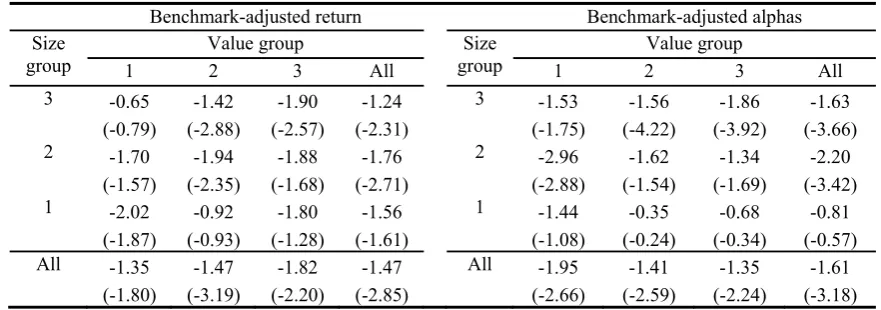
Table 2 Mutual Fund alphas

Panel A: Benchmark-adjusted returns Panel B: Four factor model alphas Panel C: Benchmark-adjusted alphas

Size group

Value group Size group

Value group Size group

Value group

1 2 3 All 1 2 3 All 1 2 3 All

3 -1.50 -1.42 -0.46 -1.29 3 -2.54 -2.25 -1.57 -2.24 3 -0.88 -1.56 -2.05 -1.44 (-0.92) (-2.88) (-0.44) (-1.83) (-2.59) (-5.80) (-2.29) (-5.41) (-0.66) (-4.22) (-2.67) (-2.51) 2 _{-2.81 -1.94 -2.53 -2.51 2 -2.18 -0.99 -0.27 -1.40} 2 _{-2.18 -1.62 -1.52 -1.90}

(-1.71) (-2.35) (-2.18) (-2.20) (-1.28) (-0.81) (-0.22) (-1.06) (-1.37) (-1.54) (-0.98) (-1.48) 1 _{-4.73 -1.76 -1.00 -2.70 1 -4.02 -1.99 -1.33 -2.56} 1 _{-2.04 -0.48 -0.22 -0.97}

(-2.03) (-1.68) (-0.80) (-2.00) (-2.54) (-2.19) (-1.33) (-2.65) (-1.08) (-0.36) (-0.13) (-0.68) All _{-2.70 -1.67 -1.14 -1.98 All -2.74 -1.90 -1.20 -2.09} All _{-1.55 -1.43 -1.39 -1.49}

(-1.76) (-3.17) (-1.48) (-2.53) (-2.38) (-3.91) (-1.79) (-3.30) (-1.29) (-2.65) (-1.92) (-2.04)

This table shows the results from the analysis of excess returns and alpha estimates for the period September 1998 to January 2009 (the out-of-sample period is

January 2002 to January 2009). Every month we calculate the excess return of each fund in our sample using daily return data. Excess return is measured in

excess of the self-designated benchmark (Panel A). We also estimate the alpha of each fund using the four – factor model (Panel B):

1( ) 2 3 4

i f i i m f i i i i

R −R = +a β R −R +β SMB+β HML+β MOM +e

as well as the four – factor model (Panel C):

* * * * * *

1( ) 2 3 4

i b i i m f i i i i

R −R =a +β R −R +β SMB+β HML+β MOM+e

Average excess returns and average alphas are computed for each month for the entire cross-section of funds in each group in the intersection of value/growth and

large/small cap strategies, and are subsequently averaged over the entire sample period. Average excess returns and average alphas are computed also for all

value to growth funds unconditional on size as well as for large to small cap funds unconditional on value/growth. Alphas are annualized. The numbers in