Absorption and Emission of Radiation by an Atomic Oscillator

Absorption and Emission of Radiation by an Atomic Oscillator

Milan Perkovac

Abstract

The theory of absorption and emission of electromagnetic radiation by an oscilla-tor consisting of the atomic nucleus and one electrically charged particle is de-duced using classical electrodynamics. In the steady state of an atom, emission and absorption of electromagnetic radiation are equal, so the atom is stable. In order to include reactive effects of electromagnetic radiation in the motion equa-tions, the Newton equation is modified by adding the radiative reaction force. This paper is an introduction to the derivation of the basic assumptions of quan-tum mechanics.

Key words: absorption, atoms, classical electrodynamics, electromagnetic

radia-tion, emission, oscillators, stability, steady state

1. INTRODUCTION

In 1904 J.J. Thompson (1857–1939) proposed a sta-tic model of the atom, and in 1911 E. Rutherford (1871–1937) proposed a dynamic model of the atom. It was hoped that any atomic phenomena could be explained by Newton’s mechanics and Maxwell’s electrodynamics.

However, two big problems remained unsolved. According to Maxwell’s electrodynamics, each accel-erated charged particle (such as an electron in Ruther-ford’s model of the atom) inevitably emits electro-magnetic radiation and therefore collapses into the nucleus.

The other problem was the atom’s discrete spec-trum, which was proved experimentally. The theories of Newton and Maxwell did not provide for such dis-continuity. Theories that cannot explain experiments are rejected, and rightly so.

Among other scientists, even the founders of mod-ern physics, M. Planck(1,2),1 and A. Einstein,(3) tried to find satisfactory answers within the classical continu-ity theories, but their attempts were futile.

It was obvious that the classical theories did not contain a principal limitation that would prevent their application down to the level of the atom. One of the last efforts to apply the classical theories to the model of the atom was made by J.H. Jeans in the early 1900s. But all presented arguments could not prevent modern physics from developing in some other direction.

However, the application of classical theories to the model of the atom is gaining ground again.(4–6) In this paper the problem of electromagnetic radiation and the atom’s instability is approached in terms of Max-well’s electrodynamics and Newton’s and Coulomb’s laws. The problem of the atom’s discrete spectrum requires two more classical laws, the law of charge and the law of momentum conservation. The problem of the atom’s discrete spectrum is elaborated in an-other paper by the same author.(7)

2. EMISSION OF ELECTROMAGNETIC RADIA-TION

Emission of electromagnetic radiation results from

electromagnetic fields emitted by accelerated electric charges(8) or generally from dynamic electric and magnetic fields (Poynting vector). We view the atom as a system consisting of a nucleus, with charge Q , and one particle, with charge q and mass m, moving in a circular orbit within a radius r at an angular

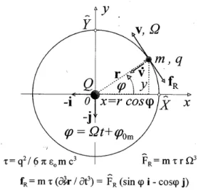
ve-locity Ω. This is Rutherford’s “planetary” model of the atom(9,10) (see Fig. 1). The distance of a particle from point x = 0 is

0 ˆ 0

( , ) cos( m) cos( m),

x Ω =t r Ω +t

ϕ

=X Ω +t

ϕ

(1)

and the distance of a particle from point y = 0 is

0 ˆ 0

( , ) sin( m) sin( m),

Figure 1. The particle of mass m and charge q rotating in a circle of radius r with velocity v and angular frequency Ω in the field of central charge Q (Rutherford’s “planetary” model of the atom). The radiative reaction force fR is, according to Wheeler

and Feynman, 90° out of phase with the acceleration v , which

means that it is perpendicular to the radius vector r and opposite to the velocity v. This force contributes to the absorption of the radiant energy and does not allow an electron to be more accel-erated and thus contributes to the stability of the atom.

where

ˆ ˆ

X Y r+ = (3)

is the amplitude of forced harmonic motion and

ϕ

0m is

a phase angle (which explains that at the moment t =

−ϕ0m

/

Ω

prior to the beginning of observation t = 0 the distance x has reached its maximum value). The radius vector r of the electron moving in the plane is

0 0

[cos( _m) sin( _m) ].

r t

ϕ

t

ϕ

= Ω + + Ω +

r i j (4)

The total emitted power of electromagnetic radia-tion, pE(t), of an electron in the atom is the sum of the

momentary power of electromagnetic radiation pEx(t)

and pEy(t) of two dipoles(11,12) at right angles to each

other, along the x and y axes of Cartesian coordinates; i.e., 2 2 4 2 0 3 0 ( ) cos ( ), 6 Ex m q r p t t c

ϕ

πε

Ω = Ω + (5) 2 2 4 2 0 3 0 ( ) sin ( ), 6 Ey m q r p t t c

ϕ

πε

Ω = Ω + (6) 2 2 4 3 0 ( ) ( ) ( ) . 6 E Ex Ey q r p t p t p t c

πε

Ω = + = (7)

The result (7) is known as the Larmor formula for radiated power,(13) an invariant of the Lorentz trans-formation.(14) _{The average power of one dipole in the}

x or y axis, PEx or P , emitted in one electron rota-Ey tion cycle, is(15,16) 2 2 4 3 0 . 12 Ex Ey q r P P c

πε

Ω = = (8)

The total average power P is the sum of _E P and _Ex

Ey P : 2 2 4 3 0 . 6 E Ex Ey q r P P P c

πε

Ω = + = (9)

We view the atom as an electromechanical oscilla-tory system. We assume that the atom has at least one stable state. Suppose the x and y components of the

driving force f acting on the electron in an atom

oscil-late sinusoidally with amplitude ˆF at particular fre-quency

ω

: 0 ˆ ( , ) cos( ), x f f

ω

t =F

ω ϕ

t+ (10) 0 ˆ ( , ) sin( ), y f f

ω

t =F

ω ϕ

t+ (11) ( , )ω t = f_x( , )ω t + f_y( , ) ,ω t f i j (12) 2 2 ˆ | ( , ) |f ω t = f_x + f_y =F, (13) where ϕ0f is a phase angle (which explains that at the

moment t = −ϕ0f/ω prior to the beginning of observa-tion t = 0 the force fx reached its maximum value). A

correct calculation must include the reaction of the elec-tromagnetic radiation on the motion of the source.(17) So, besides the Coulomb force (qQ/4πε0 r 2), which is

actually the centripetal force (mv 2_{/r), and the other}

external forces, there is another force acting on an electron, i.e., the radiative reaction force.(18–20)

Ac-cording to J.A. Wheeler and R.A. Feynman, who take up the proposition put long ago (1922) by Tetrode(21)

that the act of emission should be somehow associ-ated with the presence of an absorber, this force is

3 3 , R mτ _t ∂ = ∂ r f (14)

where τ is the characteristic time,(22),2 which will be defined later. Wheeler and Feynman made a rather general derivation of the law of radiative reaction. Consequently, expression (14) is generally accepted as correct for a slowly moving particle subjected to arbitrary acceleration. Hence the total force acting on the electron is the sum of the Coulomb force, other external forces, and the radiative reaction force.

The mechanism of electromagnetic radiation is complex(23) and not sufficiently explained.(24) In this article we consider only one atom, so no statistical mechanics(25,26) can be applied. However, a question arises now of how to include the radiative reaction force in the equation of motion. There are two possibilities. a) The sum of the radiative reaction force fR and the

external force fext is a single driving force f = fR +

fext, and the equation of motion is

. R ext

mv f= +f (14a)

b) The driving force is only the external force fext, and

the equation of motion is the Abraham–Lorentz

equation of motion

( ) _ext.

m v−τv =f (14b)

As is well known, the Abraham–Lorentz equation generated so-called runaway solutions,(27) so we opt for the first possibility. So the equation of motion based on Newton’s second law of motion, which in-cludes the resistive force and the restoring force,(28–31) is

2 0 2 ˆ cos( f), x x m +b + kx F t t t ω ϕ ∂ ∂ _{= +} ∂ ∂ (15)

or, after dividing by m and rearranging, 2 2 0 0 2 ˆ cos( _f), x₊ x _{x =}F _t t t m ω ϕ ∂ _Γ∂ _{+ Ω +} ∂ ∂ (16)

where b is the damping constant,(32) k is the spring constant,(33)

b m

Γ = (17)

is the decay constant,(34) also called the half-width or

line breadth,(35) and

0

k =

m

Ω (18)

is the angular frequency at which the simple harmonic oscillator oscillates, also called its natural

fre-quency(36) (to distinguish it from the angular fre-quency ω at which it might be forced to oscillate in steady state by a driving force f).

Using (1) and (2), we get

0 0 ˆ _{sin( m),} ˆ _{cos( m),} x y = X t = Y t t ϕ t ϕ ∂ _{− Ω Ω +} ∂ _{Ω Ω +} ∂ ∂ (19) 2 2 0 2 2 2 0 2 ˆ _{cos( ),} ˆ _{sin( ),} m m x_{= X t} t y_{= Y t} t ϕ ϕ ∂ _{− Ω Ω +} ∂ ∂ _{− Ω Ω +} ∂ (20) 3 3 0 3 3 3 0 3 ˆ _{sin( ),} ˆ _{cos( ).} m m x = X t t y = Y t t ϕ ϕ ∂ _{Ω Ω +} ∂ ∂ _{− Ω Ω +} ∂ (21)

Using (3), (4), (14), and (21), we get 3

0 0

[sin( ) cos( ) ],

R =m rτ Ω Ω +t ϕ m − Ω +t ϕ m

f i j (22)

where the amplitude of the radiative reaction force is 3

ˆ_{R .}

F =m r

τ

Ω (23)

The solution of differential equation (15) in the steady state is (1). So, from (1), (16), (19), and (20), we get 2 2 0 0 0 2 2 0 0 0 0 0

ˆ [( )sin cos ]sin

ˆ [( )cos sin ]cos

ˆ ˆ

sin sin cos cos 0.

m m m m f f X t X t F _t F _t m m ϕ ϕ ϕ ϕ ϕ ω ϕ ω Ω − Ω − ΓΩ Ω − Ω − Ω + ΓΩ Ω + − = (24)

The electron oscillates in the steady state of the atom at a particular frequency ω of the driving force f,

even if this frequency is different from the natural frequency Ω0 of the undamped oscillations.(37) So, in

the case of steady state, , ω Ω = (25) and (24) becomes 2 2 0 0 0 0 2 2 0 0 0 0 ˆ [( )sin cos ] ˆ sin sin ˆ [( )cos sin ] ˆ cos cos 0. m m f m m f X F _t m X F _t m

ω

ϕ

ω

ϕ

ϕ

ω

ω

ϕ

ω

ϕ

ϕ

ω

− Ω − Γ + − − Ω + Γ + = (26)

Equation (26) is valid for every value of t only when the coefficients of the linearly independent time-functions sin

ω

t and cos

ω

t each equal zero. So, for amplitude Xˆ , we get 2 2 2 2 2 0 ˆ ˆ _, ( ) F X m

ω

ω

= − Ω + Γ (27)

and, for a phase (

ϕ

0m −

ϕ

0f),(38,39)

0 0 2 2 0 tan(

ϕ

m

ϕ

f)

_ω

ω

, Γ − = − Ω (28)

where (

ϕ

0m −

ϕ

0f) is the phase angle between the

driv-ing force fx(

ω

, t) and the distance x(

ω

, t) [or the phase

angle between the driving force fy(

ω

, t) and the

dis-tance y(

ω

, t)], i.e., the phase angle between the driv-ing force f and the radius vector r.

If we substitute r in (8) for ˆX from (27), then the average power (8) of one dipole in an x or y axis, PEx or PEy, emitted in one cycle of electron rotation in steady state (Ω =

ω

), is (see Figs. 2 and 3)

2 4 2 3 2 2 2 2 2 2 0 0 ˆ , 12 ( ) Ex q F P c m ω πε ω ω = − Ω + Γ (29)

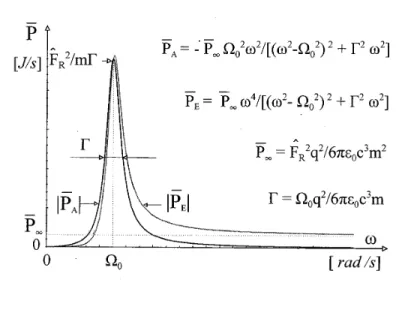
Figure 2. The total average power P_E emitted in one cycle of

particle rotation and the total average power PA absorbed in one

cycle of particle rotation, versus the frequency of external force ; the natural frequency of a particle is Ω0 and the width of an

oscillator is Γ. 2 4 2 3 2 2 2 2 2 2 0 0 ˆ , 12 ( ) Ey q F P c m ω πε ω ω = − Ω + Γ (30)

and the total average emitted power is

2 4 2 2 3 2 2 2 2 2 0 0 4 2 2 2 2 2 0 ˆ 6 ( ) , ( ) E Ex Ey E P P P q F m c P

ω

πε

ω

ω

ω

ω

ω

∞ = + = − Ω + Γ = − Ω + Γ (31) where 2 2 2 3 0 ˆ 6 E F q P m c πε ∞ = (32)

is the average power emitted in one cycle of electron rotation if the frequency ω of the external force is approaching ∞, i.e., ω → ∞.

3. ABSORPTION OF ELECTROMAGNETIC RA-DIATION

Absorption of electromagnetic radiation(40) of one dipole in the x axis results from the work of fxdx = fxvxdt = fx∂x/∂tdt = pxdt done on the charge q by the

Figure 3. Detail of Fig. 2. driving force fx: 2 2 1 1 2 1 0 0 ˆ ˆ [ cos( )][ sin( )] . t t x x t t t f m t x p dt f dt t F ω ϕt X t ϕ dt ∂ = ∂ = + − Ω Ω + (33)

So, in the same system of an atom as the one men-tioned above, the average power PAx absorbed in one cycle of driving force fx with frequency ω [because of

(25) we can also take the integral to t2 = 2π/Ω instead

of t2 = 2π/ω], using (27) and (33), in steady state (Ω = ω), is 2 1 2 1 2 2 / _{0 0} 2 2 2 2 2 0 0 2 2 2 2 2 2 2 0 2 / 0 0 0 ˆ _{cos( )sin( )} 2 _{( )} ˆ 2 ( ) cos( )sin( ) . t _{f m} Ax _t t f m t F t t P dt m F m t t dt π ω π ω ω ω ϕ ω ϕ ω π _{ω ω} ω π ω ω ω ϕ ω ϕ = = = = + + = − − Ω + Γ = − − Ω + Γ × + + (34)

The solution3 of this equation is 2 0 0 2 2 2 2 2 0 ˆ sin( ). 2 ( ) Ax m f F P m ω _{ϕ ϕ} ω ω = − − − Ω + Γ (35)

Using (28) and sin(ϕ0m − ϕ0f) = tan(ϕ0m − ϕ0f)/[1 + tan2(ϕ0m − ϕ0f)]1/2, we get 2 2 2 2 2 2 2 0 ˆ . 2 ( ) Ax F P m ω ω ω Γ = − − Ω + Γ (36)

Also, the average power P absorbed in one cycle Ay of the driving force fy is like P in (36): _Ax

2 2 2 2 2 2 2 0 ˆ . 2 ( ) Ay F P m ω ω ω Γ = − − Ω + Γ (37)

The total average absorbed power in one cycle of electron rotation is the sum of P and _Ax P_Ay:(41)

2 2 2 2 2 2 2 0 ˆ . ( ) A Ax Ay F P P P m ω ω ω Γ = + = − − Ω + Γ (38)

The sum of the total emitted and absorbed average powers, P (overall electromagnetic spectrum, if not only ω but other components of frequency in the Fou-rier series of driving forces are present), in the steady state (ω = Ω), is zero (see Fig. 3):

0

A E

P P= +P = (39)

(by the steady state, i.e., by ω = Ω). By using (31), (38), and (39), we get 2 2 3 0 , 6 q mc πε Ω Γ = (40)

and, by using (32) and (40), (38) is 2 2 2 2 2 2 2 0 . ( ) A E P P ω ω ω ∞ Ω = − − Ω + Γ (41)

4. PARAMETERS OF AN ATOMIC OSCILLA-TOR

We observe an electron on one stationary circular orbit. The centrifugal and centripetal forces of the electron in this orbit are in equilibrium. If there is any small disturbance in such a system, the electron be-comes exposed to additional radial oscillations with a small amplitude near the stationary circular orbit, i.e., near the equilibrium position. Such an amplitude is smaller than the radius of an electron orbit. So there is one electromechanical oscillator with a restoring force and parameters such as the spring constant (force constant), natural frequency, damping constant, half-width, and characteristic time. Although we do not know the size of the electron, we will determine

all these parameters. In this article it is not necessary to know the size of the electron nor the size of the nucleus. We assume that the size of the electron and the size of the nucleus are much smaller than the dis-tance between them.

(a) Spring constant and natural frequency

The next three relations (all resulting from the same equation v = Ωr) are valid for the uniform circular

motions of an electron on the radius r with angular frequency Ω and linear velocity v:

( , ) v , r Ω v = Ω (42) ( , )v r v, r Ω = (43) ( , ) . v Ω r = Ωr (44)

We assume that f∆ is the sum of all radial forces act-ing on the electron near the equilibrium position. The equilibrium position is on the circle of radius r. If the electron is moved either to one side or to the other side away from the equilibrium position, the force f∆ returns it to the equilibrium position. This force is called the restoring force.(42) _{The small magnitude of}

the restoring force df∆ is found to be directly propor-tional to the distance dr (dr being the dislocation of the electron from the equilibrium position on the ra-dius r):

.

df_∆ = −kdr (45)

We assume that in a near-equilibrium position three radial forces are acting on the electron:

2

centripetal (radial) force, d mv F r = = (46) 2 0 ,

Coulomb s law (force), 4 C qQ F r πε = = (47)

and the restoring force f∆. Thus we can write 2 2 0 0, 4 mv qQ f r πε r ∆+ + = (48) or, using (44), 2 2 0 0. 4 qQ f m r r πε ∆ + Ω + = (49)

The differential of the force f∆(Ω, r) is

[ ( , )] f f , d f r dr d r ∆ ∆ ∆ ∂ ∂ Ω = + Ω ∂ ∂Ω (50) i.e., using (49)

(

)

2 3 0 [ ( , )] 2 . 2 qQ d f r m dr m r d r

πε

∆ Ω = − Ω + + − Ω Ω(51)

The differential dΩ of angular frequency Ω according to (43) is 2 1 ( , ) v . d v r dv dr dv dr v r r r ∂Ω ∂Ω Ω = + = − ∂ ∂ (52)

The absolute value of the linear velocity v in steady state is constant, so

0.

dv= (53)

From (51), by using (43), (52), and (53), we get 2 3 2 0 [ ( , )] 2 , 2 qQ v d f r m m r dr r r

πε

∆ Ω = − Ω + + Ω (54) i.e., 2 3 0 [ ( , )] . 2 qQ d f r m dr r

πε

∆ Ω = Ω + (55)

In compliance with (45), the restoring force is df∆ = −kdr and, if we set this equal to (55), we get the

spring constant k: 2 3 0 . 2 qQ k m r πε = − Ω − (56)

So the natural frequency, (18), of an electron moving in circular atomic orbits is

2 0 3 0 . 2 k qQ m

πε

mr Ω = = −Ω − (57)

In the equilibrium state f∆ = 0 and, according to (48), we have 2 2 0 . 4 mv qQ r = − πε r (58)

Because of (43) (i.e., v/r = Ω), from (58) it follows that 2 3 0 . 4 qQ mr πε Ω = − (59)

So, from (57)and using (59), we get

2 0 3 3 0 0 . 2 4 qQ qQ mr mr

πε

πε

Ω = −Ω − = − = Ω (60)

(b) A half-width and damping constant

Relation (60) means that absorption and emission are equal in case of the condition Ω = Ω0. Any

circu-lar motion satisfies this condition. So, according to (40), Γ is also 2 2 0 3 0 , 6 q mc πε Ω Γ = (61)

and, according to (41), P is also A 2 2 0 2 2 2 2 2 0 . ( ) A E P P ω ω ω ∞ Ω = − − Ω + Γ (62)

Finally, in the equilibrium state (Ω = Ω0), from (56)

and (60), we get 3 0 , 4 qQ k r πε = − (63)

or the force constant(43) is also

2 2

0.

k m= Ω = Ωm (64)

In the steady state (ω = Ω = Ω0, ω ≠ 0, Γ ≠ 0),

accord-ing to (28), tan(ϕ0m − ϕ0f) = ∞, i.e.,

0 0 .

2

m f π

ϕ −ϕ = (65)

The radius vector r and the driving force f are at right

angles to each other (see Fig. 1). Using (10), (11), and (12), and by ω = Ω and ϕ0f = ϕ0m− π/2, the driving

force f is

0 0

ˆF[sin( t

ϕ

_m) cos( t

ϕ

_m) ] .

= Ω + − Ω +

f i j (66)

A comparison of the radiative reaction force (22) and the driving force (66) shows that the driving force f

and the radiative reaction force fR in the steady state

are two parallel forces. If there are no other external forces, the radiative reaction force is the only acting force.(44) _{So we get}

3

ˆ ˆ

R

F F= =m r

τ

Ω . (67)

Using (3), (27), and ω = Ω = Ω0, we get(45)

2_,

τ

Γ = Ω (68)

and, using (40) and (68), 2 3 0 . 6 q mc τ πε = (69) According to (17) and (68), 2_. b m= τΩ (70)

Using (60), we can show (61) in the steady state as

2 ₃ 0 1 _. 6 2 Q q m cr πε Γ = − (71)

(c) Oscillator energy and frequency

The total energy of a harmonic oscillator is(46,47)

2 2 2 2 2

1 _ˆ 1 _ˆ 1 _,

2 2 2

and, using (58) and (63), we get 2 0 1 _. 2 8 qQ E mv r πε = = − (73)

Now we have all the parameters of the atom as an electromechanical oscillator. We can now discuss other interesting relations.

We can quite freely select any of the states in an atom as the state of reference. All the variables in that state will be written with an underlined symbol. The period of one cycle of an electron is

2 1_. T π ν = = Ω (74) According to (60) and (74), 3 1 _. ( / )r r ν ν = (75)

The product of the period T and energy E of an os-cillator we call the mechanical action and denote as å = ET. According to (60), (72), (73), and (74), we get

2 0 . 4 qQ mr å ET

π

r m

π

π

rmv

ε

− = = Ω = = (76)

If we divide (76) by mv, we get πr = å/mv, the ac-tion/momentum of the particle. It resembles de Broglie’s basic postulate for the matter wave,(48) λ =

h/mv, where h is Planck’s constant. Since an electron

moves in circles, according to de Broglie’s hypothe-sis, the electron wave must be a circular standing wave with 2πr = nλ, and å should be nh/2. But for our consideration here we do not need the matter wave or Planck’s constant.

For the state of reference we have, from (76),

0 . 4 qQ mr å ET

π

π

rmv

ε

− = = = (77)

If we select the state of reference in one atom, then å is the referent mechanical action for that atom. It is the value of the fixed amount; i.e., it is a constant for that atom.

We denote the quotient of two mechanical actions as κå and, according to (76) and (77), it is

å å ET r = å ET r κ = = (78) or 2_, å r r =κ (79)

where κå is any positive real number. Obviously in

any state of reference κå = (r/r)1/2 = 1. This means

that κå is a natural number and always equals one.

From (75) and (79) we get 3, å ν ν κ = (80) and, from (78), , å ET å= =κ å (81) and (76) becomes å rmv å. π =κ (82)

Expression (82) resembles Bohr’s quantum

condi-tion(49) (2πrmv = nh). κå is a real number that can also

be any natural number n. The referent mechanical action å is a constant, as h is in Bohr’s condition. But we cannot affirm now that κå is a natural number.

This affirmation is confirmed in Ref. 7, where elec-tromagnetic properties of the atom are included.

Equations (74), (80), and (81) give 2 . å å å E κ νå ν κ = = (83)

The relation (83), E = κååν, resembles Planck’s quan-tum hypothesis(50) _{(E = nhν), which is very important}

for quantum physics. There was a lot of discussion on how to explain in terms of physics the meaning of some quantities in the relation E = nhν. However, in our relation (83) all of the quantities are completely clear in terms of physics. The basic physical differ-ence between Planck’s relation E = nhν and (83) is the meaning of frequency ν. According to Planck’s relation E = nhν, the frequency ν means the fre-quency of an electromagnetic wave νem. In relation

of mechanical rotation of an electron in the atomic orbit.

At the state of reference (where κå = 1), according

to (83), we have

.

E å= ν (84)

Notwithstanding the similarity between (84) and Ein-stein’s photon equation(51) (E = hνem), we note that ν

is not the frequency of electromagnetic oscillations in a vacuum νem (the frequency of light) but the

fre-quency of mechanical rotation of an electron in the atom’s state of reference, and this is a significant dif-ference. The physical connection between these two frequencies demands a detailed electromagnetic analysis, which is made in Ref. 7.

E3/ν2_{, according to (60), (63), (72), and (74), can be}

shown as 2 3 2 0 . 2 4 E m qQ ν = ε (85)

For a definite system (where q and Q are determinate and fixed) E3/ν2 _{is constant. We can show (85) as}

2 3 0 . 2 4 m qQ E

ν

ε

= (86)

Setting E = κååν from (83) equal to (86), we get

2 _{2 2} 3 3 2 3 3 0 0 . 2 _å 4 32 _å m qQ mq Q å å ν κ ε ε κ = = (87) If we put (87) in (86), we get 2 2 2 2 2 0 . 32 å mq Q E å ε κ = (88)

The greatest ionization potential of hydrogen(52,53) (1

1H ) is Vi = 13.5978 V. We select that state as the state of reference of the hydrogen atom. The total energy of a harmonic oscillator in that state is E = eVi

= 2.1786 × 10−18 J. So, according to (88), we can now calculate the mechanical action å in the state of refer-ence (κå = 1, |q| = |Q| = e): 34 0 | | _{3.3139 10 J s.} 4 2 qQ m å E ε − = = × ⋅ (89)

The greatest ionization potentials of 4

2He+, 73Li++, 9

4Be+++, and 115B++++ are 54.41 V, 122.414 V, 217.605 V, and 339.965 V, respectively. If we select these states as the states of reference and calculate the me-chanical actions according to (89), we get the same result for all of the elements: å = 3.3139 × 10−34 J ⋅ s (see Table I). It seems that the mechanical action in such states of reference is constant for all elements. Still it does not mean that å is a fundamental constant, because å depends on our free choice. In different states of reference å has a different value.

Setting E = mv2_{/2 and E = −qQ/8}πε_{0r, both}

ex-pressed from (73), separately equal to (88), we get

0 4 _{å å} qQ v v å ε κ κ − = = (90) and 2 2 2 0 4 å _. å å r r mqQ

ε κ

_κ

π

= − = (91)

Setting (83) equal to (88) and using (84), we get 2

3 _.

E å= νν (92)

Using (87) and (88) for the frequency difference and the energy difference of any two stationary states characterized by κå and κå′ (κå′ > κå), we get

2 2 2 3 3 3 3 3 0 1 1 1 1 32 å å å å mq Q å

ν ν ν

ν

ε

κ

κ

κ

κ

′ ∆ = − = − = − ′ ′ (93) and 2 2 2 2 2 2 2 2 0 1 1 1 1 _. 32 _{å å å å} mq Q E E E E å

ε

κ

κ

κ

κ

′ ∆ = − = − = − ′ ′ (94)

Equations (93) and (94) remind us of the well-known Bohr expression of the atomic radiant frequency(54)

and the radiant energy.(55) But there is a fundamental difference between the frequencies ν of the circular motion of the electron and the frequency of radiated electromagnetic energy νem by Bohr. The explanation

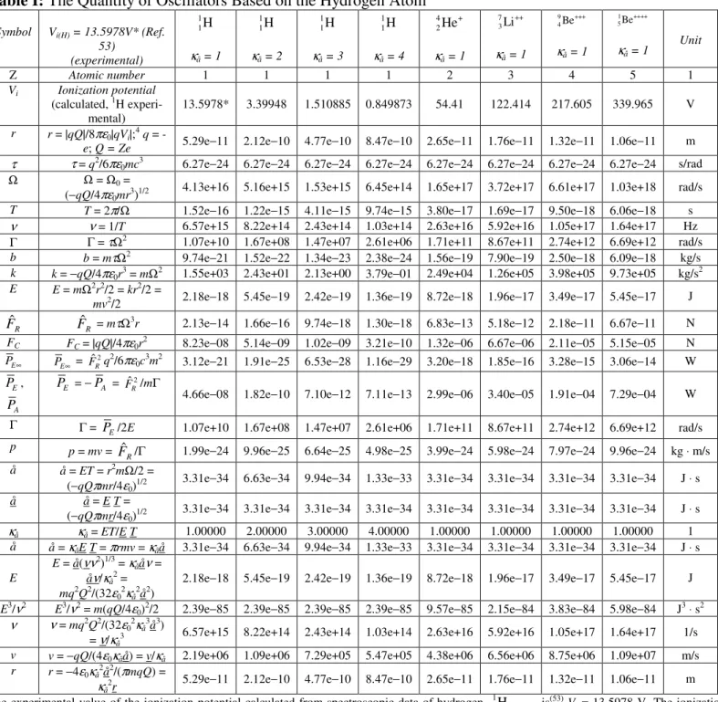
Table I: The Quantity of Oscillators Based on the Hydrogen Atom Symbol Vi(H) = 13.5978V* (Ref.

53) (experimental) 1 1H κå = 1 1 1H κå = 2 1 1H κå = 3 1 1H κå = 4 4 + 2He κå = 1 7 ++ 3Li κå = 1 9 +++ 4Be κå = 1 1 ++++ 5Be κå = 1 Unit Z Atomic number 1 1 1 1 2 3 4 5 1 Vi Ionization potential (calculated, 1_H experi-mental) 13.5978* 3.39948 1.510885 0.849873 54.41 122.414 217.605 339.965 V r r = |qQ|/8πε0|qVi|;4 q =

-e; Q = Ze 5.29e−11 2.12e−10 4.77e−10 8.47e−10 2.65e−11 1.76e−11 1.32e−11 1.06e−11 m

τ τ = q2_/6πε

0mc3 6.27e−24 6.27e−24 6.27e−24 6.27e−24 6.27e−24 6.27e−24 6.27e−24 6.27e−24 s/rad

Ω Ω = Ω0 =

(−qQ/4πε0mr3)1/2 4.13e+16 5.16e+15 1.53e+15 6.45e+14 1.65e+17 3.72e+17 6.61e+17 1.03e+18 rad/s T T = 2π/Ω 1.52e−16 1.22e−15 4.11e−15 9.74e−15 3.80e−17 1.69e−17 9.50e−18 6.06e−18 s

ν ν = 1/T 6.57e+15 8.22e+14 2.43e+14 1.03e+14 2.63e+16 5.92e+16 1.05e+17 1.64e+17 Hz Γ Γ = τΩ2 _{1.07e+10 1.67e+08 1.47e+07 2.61e+06 1.71e+11 8.67e+11 2.74e+12 6.69e+12 rad/s} b b = mτΩ2 _{9.74e−21 1.52e−22 1.34e−23 2.38e−24 1.56e−19 7.90e−19 2.50e−18 6.09e−18 kg/s} k k = −qQ/4πε0r3 = mΩ2 1.55e+03 2.43e+01 2.13e+00 3.79e−01 2.49e+04 1.26e+05 3.98e+05 9.73e+05 kg/s2 E E = mΩ2_r2_{/2 = kr}2_{/2 =}

mv2_/2 2.18e−18 5.45e−19 2.42e−19 1.36e−19 8.72e−18 1.96e−17 3.49e−17 5.45e−17 J R

Fˆ FˆR = mτΩ3r 2.13e−14 1.66e−16 9.74e−18 1.30e−18 6.83e−13 5.18e−12 2.18e−11 6.67e−11 N

FC FC = |qQ|/4πε0r2 8.23e−08 5.14e−09 1.02e−09 3.21e−10 1.32e−06 6.67e−06 2.11e−05 5.15e−05 N

E

P∞ PE∞ = F qˆR2 2/6πε0c3m2 3.12e−21 1.91e−25 6.53e−28 1.16e−29 3.20e−18 1.85e−16 3.28e−15 3.06e−14 W

E P , A P E P = −PA = F /mˆR2 Γ

4.66e−08 1.82e−10 7.10e−12 7.11e−13 2.99e−06 3.40e−05 1.91e−04 7.29e−04 W Γ _{Γ =} P_E/2E 1.07e+10 1.67e+08 1.47e+07 2.61e+06 1.71e+11 8.67e+11 2.74e+12 6.69e+12 rad/s

p _{p = mv =}

R

Fˆ /Γ 1.99e−24 9.96e−25 6.64e−25 4.98e−25 3.99e−24 5.98e−24 7.97e−24 9.96e−24 kg ⋅ m/s å å = ET = r2_{mΩ/2 =}

(−qQπmr/4ε0)1/2 3.31e−34 6.63e−34 9.94e−34 1.33e−33 3.31e−34 3.31e−34 3.31e−34 3.31e−34 J ⋅ s

å å = E T =

(−qQπmr/4ε0)1/2 3.31e−34 3.31e−34 3.31e−34 3.31e−34 3.31e−34 3.31e−34 3.31e−34 3.31e−34 J ⋅ s κå κå = ET/E T 1.00000 2.00000 3.00000 4.00000 1.00000 1.00000 1.00000 1.00000 1

å å = κåE T = πrmv = κåå 3.31e−34 6.63e−34 9.94e−34 1.33e−33 3.31e−34 3.31e−34 3.31e−34 3.31e−34 J ⋅ s

E E = å(νν2₎1/3 _{= κ} ååν = åν/κå2 = mq2_Q2_/(32ε 02κå2å2)

2.18e−18 5.45e−19 2.42e−19 1.36e−19 8.72e−18 1.96e−17 3.49e−17 5.45e−17 J E3_/ν2 _E3_/ν2 _{= m(qQ/4ε}

0)2/2 2.39e−85 2.39e−85 2.39e−85 2.39e−85 9.57e−85 2.15e−84 3.83e−84 5.98e−84 J3 ⋅ s2 ν ν = mq2_Q2_/(32ε

02κå3å3)

= ν/κå3 6.57e+15 8.22e+14 2.43e+14 1.03e+14 2.63e+16 5.92e+16 1.05e+17 1.64e+17 1/s

v v = −qQ/(4ε0κåå) = v/κå 2.19e+06 1.09e+06 7.29e+05 5.47e+05 4.38e+06 6.56e+06 8.75e+06 1.09e+07 m/s

r r = −4ε0κå2å2/(πmqQ) =

κå2r 5.29e−11 2.12e−10 4.77e−10 8.47e−10 2.65e−11 1.76e−11 1.32e−11 1.06e−11 m

The experimental value of the ionization potential calculated from spectroscopic data of hydrogen, 1₁H₍κ_å=₁₎, is(53) Vi = 13.5978 V. The ionization

potentials of 1₁H₍κ_å=₂₎, 11H(κå=3), 1 1H(κå=4), 4 + 2He (κå=1), 7 ++ 3Li (κå=1), 9 +++ 4Be (κå=1), and 11 ++++

5Be (κå=1) are calculated here in such a way that the quotient of mechanical actions of each atom, κå = ET/E T, becomes a natural number. Without additional criteria, κå can theoretically be any rational

number.

The energy ∆E in (94) and the energy of the

elec-tromagnetic wave 2 ( ) 2 2 2 2 1 1 8 em mc E n n

π γ

∆ ≈ − _′ (95)

in Ref. 7 are identical (the atom-structure coefficient γ is nearly constant; n and n′ are positive integers). So

mq2Q2/32ε02å2 = mc2/8π2γ2, and we get 0 0 | | 1 _{| |,} 2 2 e å qQ å Z qQ c π _π γ ε = = = (96)

where Z0 = 1/ε0c = 376.7303 Ω. We call å/γ the

ele-mentary action and denote it as åe. In the case of

× 10−34 J ⋅ s. It is 21.81 times less than the referent

mechanical action å according to (89), and 43.62 times less than the Planck constant h. The elementary action åe = 1/2πZ0e2 is a universal physical constant. 5. CONCLUSION

An electric charge emits electromagnetic energy whenever it is accelerating. Thus an electron that ro-tates around the nucleus, with a constant centripetal acceleration, constantly emits electromagnetic energy. Consequently, its energy should diminish gradually. This would lead to a gradual reduction in the dimen-sions of its orbit so that the electron would finally fall into the nucleus.(56)

However, at the same time there is a process in the atom working in the opposite direction. Generally, an electron in the atom is also absorbing electromagnetic radiation. Indeed, it is the radiative reaction force that by emission of electromagnetic radiation in a steady state contributes to the absorption of electromagnetic

radiation in the atom. This means that in the atom’s steady state this absorption is equal to the emission of electromagnetic radiation, and the atom remains stable.

In this article the atom is treated as an electrome-chanical oscillator. All the parameters of this oscilla-tor are determinate: characteristic time τ, damping con-stant b, spring concon-stant k, half-width Γ, and natural fre-quency Ω0. Emission of electromagnetic radiation in the

atom’s steady state was a fundamental argument against applying classical electrodynamics to it. According to this article, such objections no longer hold ground.

On the basis of mechanical considerations, this arti-cle lays the foundations for a deduction of Planck’s quantum hypothesis, Einstein’s photon equation, Bohr’s quantum condition, and de Broglie’s hypothe-sis, whereas the details of quantization are given by the same author in another article(7) by including the others’ electromagnetic consideration.

Received 28 March 2001.

Résumé

La théorie de l’absorption et de l’émission de la radiation électromagnétique d’un oscillateur composé du noyau atomique et d’une particule électriquement chargée est déduite en utilisant l’électrodynamique classique. En état stationnaire d’un atome, l’émission et l’absorption de la radiation électromagnétique sont égales, donc, l’atome est stable. Afin d’intégrer les effets réactifs de la radiation dans l’équation du mouvement, l’équation de Newton est modifiée en ajoutant la force de réaction radiative. L’article présente une introduction à la déduction des propositions de base de la mécanique quantique.

Endnotes

1 _{“The question as to whether the rays of light are}

quantized or the quantum effect originates only in-side the matter is indeed just the first and toughest dilemma the whole quantum theory is faced with and the answer to that question is still to direct its further development.” (In the original: “ … In der Tat ist die Frage, ob die Lichtstrahlen selber gequantelt sind, oder ob die Quantenwirkung nur in der Materie stattfindet, wohl das erste und schwerste Dilemma, vor das die ganze Quanten-theorie gestellt ist und dessen Beantwortung ihr erst die weitere Entwicklung weisen wird.” Lecture “Das Wesen des Lichts,” 28 October 1919.)

2 _{“It is useful to note that the longest characteristic}

time τ (τ = e2/6πε0mc3) for charged particles is for electrons and that its value is τ = 6.26 × 10−24 sec.

This is of the order of time taken for light to travel 10−15 m. Only for phenomena involving such dis-tances or times will we expect radiative effects to play a crucial role.”(22) This statement shows us that classical analyses are used with systems for which mass m approaches the electron mass and charge q approaches the electron charge e.

3 _{The results and the figures in the text are generated}

by Wolfram Research, Mathematica, courtesy of Systemcom, Zagreb, Croatia.

4 _{The radii of the orbits of hydrogen are computed}

by means of the ionization potential(57) Vi

accord-ing to the relativistic formula

2 0 0 | | . 4 | i|[1 1/(1 | i| / )] qQ r qV qV m c πε = + +

References

1. M. Planck, Wege zur Physikalischen Erkenntnis (Verlag von S. Hirzel in Leipzig, 1944), p. 96. 2. E.H. Wichmann, Quantum Physics

(McGraw-Hill, New York, 1971), p. 26.

3. G.E. Tauber, Albert Einstein’s Theory of General

Relativity (Globus/Zagreb, 1984), pp. 233, 241.

4. H. Sallhofer, Naturforsch. 45a, 1361 (1990).

5. V.M. Simulik and I.Yu. Krivsky, Adv. Appl. Cliff. Algebra 7, 25 (1997).

6. Idem, Ann. Fond. L. de Broglie 27, 303 (2002).

7. M. Perkovac, Phys. Essays 15, 41 (2002).

8. F.K. Richtmyer, E.H. Kennard, and T. Lauritsen,

Introduction to Modern Physics (McGraw-Hill,

New York, 1955), p. 221.

9. D.C. Giancoli, Physics, 2nd edition (Prentice-Hall, Englewood Cliffs, NJ, 1988), p. 878.

10. H. Hänsel and W. Neumann, Physik (Spektrum, Akad. Verl., Heidelberg, Berlin, 1995), p. 81. 11. E.W. Schpolski, Atomphysik, Teil I (VEB

Deutscher Verlag der Wissenschaften, Berlin, 1979), pp. 217, 235.

12. L.D. Landau and E.M. Lifschitz, Lehrbuch der

Theoretischen Physik, Babd II, Klassische Feld-theorie, 6th edition (Akademie-Verlag, Berlin,

1973), p. 205.

13. J.D. Jackson, Classical Electrodynamics, 2nd edition (John Wiley & Sons, New York, 1975), p. 659.

14. L. Page and N.I. Adams, Electrodynamics, 2nd printing (Van Nostrand, New York, 1945), p. 328.

15. Ref. 11, p. 217.

16. H. Czichos, HÜTTE, Die Grundlagen der

In-genieurwissenschaften (Springer-Verlag, Berlin,

Heidelberg, 1989), p. B 198. 17. Ref. 13, p. 780.

18. J.A. Wheeler and R.P. Feynman, Rev. Mod. Phys. 17, 157 (1945), p. 162. 19. Ref. 13, p. 784. 20. Ref. 12, p. 238. Milan Perkovac Drives-Control P.O. Box 125 HR-10001 Zagreb, Croatia e-mail: [email protected] 21. H. Tetrode, Z. Phys. 10, 317 (1922). 22. Ref. 13, p. 782. 23. Ref. 18, pp. 158–159. 24. Ref. 13, p. 781.

25. V.A. Fok, Dokl. Akad. Nauk. 60, 1157 (1948).

26. S. Watanabe, Rev. Mod. Phys. 27, 26, 40, 179

(1955).

27. Ref. 13, p. 784. 28. Ref. 9, p. 341. 29. Ibid., p. 783.

30. J. Derzi ski and C. Gérard, Scattering Theory of

Classical and Quantum N-Particle Systems

(Springer, Berlin, Tokyo, 1997), p. 13. 31. Ref. 13, p. 802. 32. Ref. 9, p. 339. 33. Ibid., p. 326. 34. Ref. 13, p. 799. 35. Ibid., p. 800. 36. Ref. 9, p. 330. 37. Ibid., p. 341. 38. Ibid. 39. Ref. 16, p. B 30/31. 40. Ibid., p. B 32. 41. Ibid. 42. Ref. 9, p. 325. 43. Ref. 13, p. 807. 44. Ibid., p. 783. 45. Ibid., p. 807. 46. Ref. 16, p. B 27. 47. Ref. 10, p. 166.

48. L. de Broglie, Ann. Phys. 3, 22 (1925).

49. Ref. 9, p. 880. 50. Ibid., p. 869. 51. Ibid. 52. Ibid., p. 882. 53. Ref. 8, p. 167. 54. Ref. 9, p. 883. 55. Ibid., p. 881.

56. J. Orear, Physik (Carl Hanser Verlag, München, Wien, 1987), pp. 461, 462.

57. Ref. 8, p. 167.