arXiv:2004.10622v3 [math.DG] 13 Jan 2021
On Area Growth in Sol
Richard Evan Schwartz
∗January 14, 2021
Abstract
Let Sol be the 3-dimensional solvable Lie group whose underlying space isR3 and whose left-invariant Riemannian metric is given by
e−2zdx2+e2zdy2+dz2.
We prove that the sphere of radius r in Sol has surface area at most 20πer provided that r is sufficiently large. This estimate is sharp up to a factor of 10.
1
Introduction
Sol is one of the 8 Thurston geometries [Th], the one which uniformizes torus bundles which fiber over the circle with Anosov monodromy. Sol has been studied in various contexts: coarse geometry [EFW], [B]; minimal surfaces [LM] (etc.); its geodesics [G], [T], [K], [BS]; connections to Hamiltonian systems [A], [BT]; and finally virtual reality [CMST]. Our paper [CS] has a more extensive discussion of these many references.
In [CS], Matei Coiculescu and I give an exact characterization of which geodesic segments in Sol are length minimizers, thereby giving a precise de-scription of the cut locus of the identity in Sol. As a consequence, we proved that the metric spheres in Sol are topological spheres, smooth away from 4 singular arcs. We will summarize the characterization in §2 and explain the main ideas in the proof in §4.
Ian Agol recently pointed out to me that our exact characterization of the cut locus in Sol might help us determine the growth rate in balls in Sol. Eryk Kopczy´nski pointed out a rather easy calculation that Vr ≤ Cr2er for
some constant C, and this implies that Sol has volume entropy 1. See §2.8. Marc Troyanov recently showed me a preprint with the estimate Vr <8rer.
We will get finer information.
To state our main result, we normalize the metric in Sol so that it is:
e−2z
dx2+e2zdy2+dz2. (1)
In this metric the planes X = 0 andY = 0 have sectional curvature −1. Let Sr denote any metric sphere of radiusr in Sol. LetAr denote the area ofSr
with respect to the Riemannian metric in Sol.
Theorem 1.1 Ar<20πer provided that r is sufficiently large.
Remarks:
(i) Given the 2-to-1 locally-area-decreasing projection from Sr onto the
hy-perbolic disk of radius r, we have Ar > 4π(cosh(r)−1) ≈ 2πer. Thus, our
estimate is sharp up to a factor of 10.
(ii) Our analysis does not give an effective estimate on what “sufficiently large” means. However, we notice that all the relevant quantities seem to stabilize pretty quickly: one sees all the phenonena already when looking at a sphere of radius 8 in Sol.
The basic idea of the proof is to bound the projections of the sphere into the coordinate planes. Let ΠX denote the coordinate plane X = 0. Let ηX
denote the projection of Sol into ΠX. Let AX,r denote the area of ηX(Sr).
Let NX,r denote the smallest integer such that the map ηX :Sr →ΠX is at
most NX,r-to-1. We make all the same definitions withY and Z in place of
X. We also make a more refined definition for Z. Let Sr,k denote the subset
whereηZ isk-to-1, We letAZ,r,kdenote the area ofηZ(Sr,k). In§2.7 we prove
the following result.
Lemma 1.2 (Projection) For any ǫ >0 and any θ ∈(0,1)we may take r
sufficiently large so that
Ar < (NX,rAX,r+NY,rAY,r) θ−ǫ + 1 √ 1−θ2−ǫ ∞ X k=1 kAZ,k,r.
Remark: A similar result would be true for any surface in Sol which is al-most everywhere smooth, but the formula in general would not be quite as good. We use special properties of Sr to get the formula above.
We then establish the following projection estimates: 1. AX,r =AY,r = 2π(cosh(r)−1)< πer.
2. NX,r =NY,r = 2.
3. AZ,r <16∗er for sufficiently larger.
4. NZ,r = 4 for sufficiently large r.
5. AZ,k,r <0∗er for k = 3,4.
The number ζ∗
is a number we can make as close as we like to ζ by taking
r sufficiently large. Estimates 4 and 5 together combine to say that the projection ηZ is essentially 2-to-1, because the set where it is either 3-to-1 or
4-to-1 has negligible area in comparison to er. When we apply the result in
Lemma 1.2 we see that, for r large,
Ar < min θ∈(0,1) 4∗ π θ + 32∗ √ 1−θ2 er <20πer. (2) The minimizer is quite close to θ = 3/5 and the minimum is about 60.93er.
Projection Estimates 1 and 2 are straightforward given our description of the Sol spheres. Projection Estimate 3 relies on an analysis of an ODE studied in [CS] and some easy asymptotic results about elliptic functions. After giving our upper bound we will explain, a bit sketchily, why
AZ,r >(2/1∗)er
once r is sufficiently large. We do this to point out that our upper bound is fairly tight. When we plug in this smaller estimate into the Projection formula above, we get a bound of about 7πer. Ths represents a kind of
absolute limit to the strength of our method.
The hard work in the paper involves dealing with Projection Estimate 4, even though the result is clear from the computer plots such as Figure 5.4, involves a careful asymptotic study of the ODE just mentioned. Projection Estimate 5 comes out as a byproduct of our analysis.
• In §2 we introduce some preliminary material and in particular recall the Main Theorem from [CS]. We use this result to prove the Projection Lemma, though we also point out that one can prove the Projection Lemma knowing a much softer result about the Sol spheres.
• In §3, we prove Projection Estimates 1 and 2.
• In §4, we give details about the proof of the Main Theorem in [CS]. These details are needed for the proof of Projection Estimates 3 – 5.
• In §5 we give more information about the central ordinary differential equations which arise in [CS].
• In §6 we prove Projection Estimates 3 – 5 modulo the detail that a certain curve in the plane is smooth and regular except at a single cusp. See Figure 5.3. Proving this result, which we call the Embedding Theorem, turns out to be a fight with the OEDs introduced in §5.
• In §7 we prove the Embedding Theorem modulo a detail which we call the Monotonicity Lemma, a statement about the ODE from §4.3.
• in §8-9 we prove the Monotonicity Lemma. This is where all the ODE calculations come in.
I would like to thank Ian Agol, Matei Coiculescu, Justin Holmer, An-ton Izosimov, Boris Khesin, Eryk Kopczy´nski, Mark Levi, Benoit Pausader, Pierre Pansu, and Marc Troyanov for helpful discussions concerning this pa-per. I would also like to acknowledge the support of the Simons Foundation, in the form of a 2020-21 Simons Sabbatical Fellowship, and also the support of the Institute for Advanced Study, in the form of a 2020-21 membership funded by a grant from the Ambrose Monell Foundation.
2
Preliminaries
2.1
Basic Properties of Sol
The underlying space for Sol is R3. The metric is:
e−2zdx2+e2zdy2+dz2. (3) The group law on Sol is
(x, y, z)∗(a, b, c) = (eza+x, e−zb+y, c+z). (4)
Left multiplication is an isometry. We identify R3 with the Lie algebra of
Sol in the obvious way. (See [CS, §2.1] if this does not seem obvious.) Sol has 3 interesting foliations.
• The XY foliation is by (non-geodesically-embedded) Euclidean planes.
• The XZ foliation is by geodesically embedded hyperbolic planes.
• The YZ foliation is by geodesically embedded hyperbolic planes. The complement of the union of the two planes X = 0 and Y = 0 is a union of 4sectors. One of the sectors, the positive sector, consists of vectors of the form (x, y, z) with x, y > 0. The sectors are permuted by the Klein-4 group generated by isometric reflections in the planesX = 0 andY = 0. The Riemannian exponential map E preserves the sectors. Usually, this symme-try will allow us to confine our attention to the positive sector.
Notation: For each W ∈ {X, Y, Z}, the plane ΠW is given by W = 0 and
the map ηW : Sol→ΠW is the projection onto ΠX obtained by just dropping
the W coordinate. We also let πZ denote projection onto the Z-axis. Thus,
πZ(x, y, z) = z.
2.2
Properties of the Hyperbolic Slices
We discuss our results for ΠY. There are analogous results for ΠX. Here is
a basic property of the hyperbolic slices in Sol. The map F(x,0, z) = (x, ez)
converts the metric in ΠY to the standard hyperbolic metric in the upper
half plane, namely
Lemma 2.1 In ΠY, the points (0,0,0) and (dr,0,0) are connected by a
geodesic segment of length r when dr =er/2−e−r/2.
Proof: Here dr = 2 sinh(r/2). Let F be the transformation from ΠY
to the standard upper half plane model. We have F(0,0,0) = (0,1) and
F(dr,0,0) = (dr,1). As is well known, the distance between these points in
the standard hyperbolic metric is 2 sinh−1(dr/2) = 2(r/2) =r. ♠
Lemma 2.2 In ΠY, the point(x,0, z)lies in the disk of radius r centered at
(0,0,0)only if |x| ≤(er−e−r)/2.
Proof: We use the transformation F again. Looking in the standard upper
half plane model, the disk we are interested in, Dr, is centered at (0,1) and
has radius r. The two points (0, e−r) and (0, er) lie in the boundary of D r.
Hence Dr has Euclidean radius (er−e−r)/2. ♠
2.3
The Disk Lemma
Here we recall a result from topology. This result will be useful, in §5, when we prove Projection Estimate 4.
Lemma 2.3 (Disk) Let ∆ ⊂ R2 be a disk. Let h : ∆ → R2 be a map
which is a local diffeomorphism on the interior such that h(∂∆)is a piecewise smooth curve having finitely many self-intersections. Given p∈R2−h(∆),
the number of preimages h−1(p) equals the unsigned number of times h(∂∆)
winds around p.
Proof: This is a well-known result. Here we sketch the proof. Without loss
of generality, we can assume that ∆ is the unit disk in R2 and h(0,0) 6=p.
Let ∆s denote the disk of radius r centered at (0,0). Also, we can assume
that h is orientation preserving in the interior of ∆. Let f(s) denote the number of timesh(∆s) winds aroundp. For snear 0, we have f(s) = 0. The
function f changes by ±1 each time ∆s crosses a point off−1(p). The sign
is always the same because h is orientation preserving. Hence the number of points in f−1(p) equals f(1), up to sign. ♠
2.4
Elliptic Functions
Many of the quantities associated to Sol are expressed in terms of elliptic integrals. Our functions Kand E are precisely EllipticKand EllipticEin
Mathematica [W].
Basic Definition: The complete elliptic functions of the first and second
kind are given by K(m) = Z π/2 0 dθ p 1−msin2θ, E(m) = Z π/2 0 q 1−msin2(θ) dθ. (5)
The first integral has domainm ∈[0,1) and the second has domainm∈[0,1].
Differential Equations: These functions satisfy the following differential
equations. For a proof see any textbook on elliptic functions.
dK dm = (m−1)K+E 2m−2m2 , dE dm = −K+E 2m . (6)
AGM Identity: We have the following classic identity.
K(m) = π/2
AGM(√1−m,1), m ∈(0,1). (7) See [BB] for a proof.
Asymptotics: It follows directly from the definition and an elementary
integral that
E(1) = 1. (8) We also have the following:
K(m) + 12log 1−m 16 < 1−8m ×log 1−m 16 . (9) Both sides tend to 0 as m → 1. This inequality comes from the second inequality (the upper bound) in Inequality 19.9.2 of the Digital Library of Mathematical Functions: 1 + (k ′ )2 8 < K(k) log(4/k′) <1 + (k′ )2 4 . Here m = k2 and 1−m = (k′
)2. Making the substitution of m and 1−m
for k and k′
2.5
The Hamiltonian Flow
LetG= Sol. Let S1 ⊂R3 denote the unit sphere. at the origin in G. Given
a unit speed geodesic γ, the tangent vector γ′
(t) is part of a left invariant vector field on G, and we letγ∗
(t)∈S1 be the restriction of this vector field
to (0,0,0). In terms of left multiplication on G, we have the formula
γ∗
(t) =dLγ(t)−1(γ′(t)). (10)
It turns out that γ∗
satisfies the following differential equation.
dγ∗ (t)
dt = Σ(γ
∗
(t)), Σ(x, y, z) = (+xz,−yz,−x2 +y2). (11) This is explained one way in [G] and another way in [CS,§5.1]. (Our formula has a different sign than Grayson’s, because our group law correspondingly differs by a sign.) This system in Equation 11 is really just geodesic flow on the unit tangent bundle of Sol, viewed in a left-invariant reference frame.
Let F(x, y, z) = xy. The flow lines of Σ lie in the level sets of F, and indeed Σ is the Hamiltonian flow generated by F. Most of the level sets of F are closed loops. We call these loop level sets. With the exception of the points in the planes X = 0 and Y = 0, and the points (x, y,0) with |x|=|y|=√2, the remaining points lie in loop level sets.
Each loop level set Θ has an associatedperiod L=LΘ, which is the time
it takes a flowline – i.e., an integral curve – in Θ to flow exactly once around. Equation 12 below gives a formula. We can compare L to the length T of a geodesic segment γ associated to a flowline that starts at some point of Θ and flows for time T. We call γ small, perfect, or large according as T < L, or T =L, or T > L. In [CS, §5] we prove the following result:
Theorem 2.4 Suppose(x, y, z)∈S2 lies in a loop level set. Let α=p|xy|.
Then the period of the loop level set containing (x, y, z) is
Lα = π AGM(α,1 2 √ 1 + 2α2) = 4 √ 1 + 2α2 × K 1−2α2 1 + 2α2 (12) The second identity is Equation 7. Using Equation 9 we see that the differ-ence between Lα and −4 log(α/2) tends to 0 as α →0.
Each vector V = (x, y, z) simultaneously corresponds to two objects:
• The geodesic segment γV ={E(tV)| t∈[0,1]}.
Given a vector V = (x, y, z) we define
µ(V) = AGM(√xy,1
2 p
(|x|+|y|)2+z2). (13)
We call V small,perfect, orlarge according asµ(V) is less than, equal to, or greater than π. In view of Equation 12 here is what this means:
• IfγV lies in the planeX = 0 orY = 0 thenV is small becauseµ(V) = 0.
• If V = (x, y,0) where |x| = |y| then V is small, perfect, or large according as |x|< π, |x|=π or|x| ≥π.
• In all other cases, V /kVklies in a loop level set, andV is small, perfect, or large according as µ(V)< π,µ(V) =π, or µ(V)> π.
2.6
The Main Result
Now we recall the main result from [CS].
Theorem 2.5 Given any vector V, the geodesic segment γV is a distance
minimizing geodesic if and only if µ(V) ≤ π. That is, γV is distance
mini-mizing if and only ifV is small or perfect. Moreover, ifV andW are perfect vectors then E(V) = E(W) if and only if V = (x, y, z) and W = (x, y,±z).
Theorem 1.1 identifies the cut locus of the identity in Sol with the set of perfect vectors. The Riemannian exponential map E is a global diffeomor-phism on the set of small vectors. Also, E is generically 2-to-1 on the set of perfect vectors. We will explain this last fact below.
Theorem 1.1 leads to a good description of the Sol metric sphere Sr of
radius r. Let Sr denote the Euclidean sphere of radius r centered at the
origin of R3. Let
Sr′ =µ
−1
[0, π]∩Sr. (14)
The space S′
r is a 4-holed sphere. The boundary ∂S
′
r, a union of 4 loops, is
precisely the set of perfect vectors contained in Sr. Each of these loops is
homothetic to one of the loop level sets on the unit sphere S2. The Klein-4
It follows from the Main Theorem thatSr=E(Sr′) and thatE is a
diffeo-morphism when restricted to S′
r−∂S
′
r. On∂S
′
r, the mapE is a 2-to-1 folding
map which identifies partner points within each component. Thus, we see that Sr is obtained from a 4-holed sphere by gluing together each boundary
component (to itself) in a 2-to-1 fashion. This reveals Sr to be a topological
sphere which is smooth away from the set E(∂S′
r). We also prove that the
singular set E(∂S′
r) consists of 4 arcs of hyperbolas, all contained in ΠZ.
The Lunar Principle: Given a unit normal vector V to Sr at a smooth
point, we let V∗ denote the left translate of V to the origin. Let Nr denote
the set of all such vectorsVr. Given the nature of the loop level sets, we have
the following corollary of Theorem 2.5. For any ǫ > 0 there is some R such thatNr is contained in theǫ-tubular neighborhood of ΠX∪ΠY provided that
r > R. We call this theLunar Principle because ΠX∪ΠY intersects the unit
sphere in a union of 4 spherical lunes. One does not really need the full force of Theorem 2.5 to deduce the Lunar Principle: A long geodesic tangent to a unit vector that is far from ΠX ∪ΠY makes a corkscrew-like pattern and is
quite far from distance minimizing.
2.7
Proof of the Projection Lemma
We call a map η between surfacesθ-good ifarea(η(S)) area(S) ≥δ
for any measurable subset S in the domain. Mostly we are interested in the case when the domain is a smooth surface in Sol and the range is one of the coordinate planes in Sol. However, in the first result, we will consider planar surfaces in R3. The same projections ηX, ηY, ηZ make sense as projections
in R3.
Lemma 2.6 Let ΘX,ΘY,ΘZ be positive numbers with Θ2X + Θ2Y + Θ2Z = 1.
Let Π be any plane in R3. Then there is an I ∈ {X, Y, Z} such that the ηI
is ΘI-good.
Proof: It follows from the familiar fact that kV ×Wk computes the area of
Theorem, that there are 3 non-negative numbers rX, rY, rZ ≥ 0 so that
r2
X +r2Y +rZ2 = 1, and
AΠ(S) = rXAX(S) +rYAY(S) +rZAZ(S). (15)
Here S ⊂ Π is any measurable set and AX(S) is the area of ΠX(S), etc. If
our claim is false then ΘI < rI for all I ∈ {X, Y, Z}. But then
1 = Θ2X + Θ2Y + Θ2Z < rX2 +rY2 +r2Z = 1,
and we have a contradiction. ♠
Now we move the discussion to Sol.
Lemma 2.7 Let ΘX,ΘY,ΘZ be positive numbers with Θ2X + Θ2Y + Θ2Z = 1.
Let Σ be a smooth surface in Sol. Let p ∈ Σ be any point. Then for any
ǫ > 0 there is a sufficiently small neighborhood U about p and some index
I ∈ {X, Y, Z} such that ηI isΘI-good on U.
Proof: Given that Sol is homogeneous, and that the projections between
parallel planes within the same coordinate foliation are area preserving, it suffices to prove our result when p is the origin in Sol. But, in this case, the metric on Sol agrees with the Euclidean metric up to any given ǫwe like. So, this special case follows from Lemma 2.6 and the differentiability of Σ. ♠
Now let us apply the Lunar Principle to the sphereSr. Given a smooth
point p ∈ Sr, the corresponding vector Np,0 lies quite near ΠX ∪ΠY. The
reason is that Np,0 either lies in ΠX∪ΠY or else in a loop level set of period
greater than r, and such loop level sets lie near ΠX ∪ΠY. Therefore, given
any ǫ > 0 we can take r large enough so that there is a partition of the smooth points of Sr into 3 measurable (or indeed piecewise smooth) regions
Sr(I), I ∈ {X, Y, Z}
with the following properties:
• The projection ηX :Sr(X)→ΠX is (θ−ǫ) good.
• The projection ηY :Sr(Y)→ΠY is (θ−ǫ) good.
• The projection ηZ :Sr(Z)→ΠZ is (
√
1−θ2−ǫ)-good.
Since the non-smooth subset ofSr has area 0, the formula in the Projection
2.8
A Weaker Bound on Volume
This section is independent from the rest of the paper. Here we present, with minor modifications, Eryk Kopczy´nski’s derivation of a weaker volume growth bound that is still sufficient to establish that Sol has volume entropy 1. I did not try for optimal constants.
Lemma 2.8 Suppose γ is a geodesic in Sol having length r. Let r1 be the
length of γ that lies above the plane Z = 0 and let r2 be the length of γ that
lies below or in the plane Z = 0. Then the endpoint (x, y, z) of γ satisfies the bound |x| ≤er1 +r
2 and |y|< er2 +r1.
Proof: We first consider two special cases. If γ stays above the plane ΠZ
then the endpoint (x, y, z) satisfies the bounds |x| ≤ er and |y| ≤ r.
Like-wise, if γ stays below the plane ΠZ then the endpoint (x, y, z) satisfies the
bounds |y| ≤ er and |x| ≤ r. In general, one can break γ into intervals
γ1, ..., γk, for some k, such that eachγj satisfies one of the two special cases
just considered. Adding up the bounds from the special cases, we get the result advertised in the lemma. ♠
Set u=er. Note that r < u. Every point (x, y, z) in the ball of radius r
satisfies
|x|,|y| ≤u+r, |z| ≤r, (|x| −r)(|y| −r)≤u.
Let Ωr be the set of points satisfying these inequalities. For convenience we
take r ≥1 The volume of the part of Ωr where |x| ≤r+ 1 is bounded by
8r×(r+ 1)×(u+r)<32r2u.
Likewise, the volume of the part of Ωr where|y| ≤r+ 1 is bounded by 32r2u.
The volume of the part of the Ωr where |x|> r+ 1 and |y|> r+ 1 is
8r Z u 1 u x dx≤8rulog(u) = 8r 2u.
Therefore Ωr has volume at most 72r2er. But the ball of radiusris contained
3
The Hyperbolic Projections
3.1
A Picture
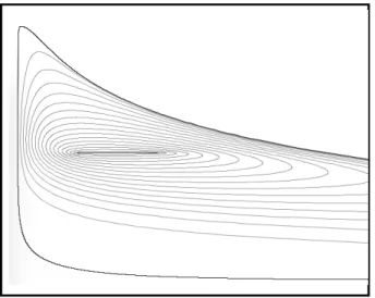
Recall thatηX : Sol→ΠX is the orthogonal projection onto the planeX = 0.
Figure 3.1 shows the projection of (part of) the positive sector of the sphere S5 into the plane ΠX. The smooth part of this sphere has a foliation by
the images of the loop level sets under the Riemannian exponential map E. The grey curves are the projections of this foliation into ΠX. The black line
segment is the projection of the set of singular points.
Figure 3.1: Projection into the plane ΠX.
It appears from the picture that the restriction of ηX to this sector is
a homeomorphism onto its image. We will prove this result below. For convenience we take r > π√2.
3.2
Area Bound
In this section we prove Projection Estimate 1. By symmetry, it suffices to prove the result for the projection ηX into the plane ΠX. Let S+r denote the
subset of Sr consisting of points (x, y, z) with x ≥ 0. Let Hr denote the
hyperbolic disk of radius r contained in the plane ΠX and centered at the
origin. All the points in the interior of S+
r lie in the open positive sector.
Because ΠX is a totally geodesic plane in Sol, we have ∂S+r = ∂Hr. The
Lemma 3.1 ηX maps the interior of S+r into the interior of Hr.
Proof: If this is false, then there is a geodesic segment γ of length r,
con-necting (0,0,0) to some point p∈ S+
r which remains entirely in the positive
sector except for its initial point, (0,0,0). The projection mapηX is distance
non-increasing, and locally distance decreasing on any curve whose tangent vector is not in a plane of the form X = const.. This means that ηX(γ) is
shorter than γ. But then ηX(γ) cannot reach the point ηX(p)∈∂Hr. ♠
3.3
Multiplicity Bound
In this section we prove Projection Estimate 2. As above, it suffices to prove this result for the projection ηX into the plane ΠX. To prove that NX,r = 2
it suffices, by symmetry, to show thatηX is an injective map fromS+r to ΠX.
The basic strategy is to show that ηX is locally injective. We also know that
ηX is the identity on the boundary of S+r, which already lies in the plane
X = 0. (It is the boundary of the hyperbolic disk on ΠX of radius rcentered
at the origin.) Our injectivity result then follows from the Disk Lemma in
§2.
For convenience we take r > π√2 in the next result, so that we don’t have to discuss several cases. (The sphereSr is smooth forr < π
√
2 and has 4 singular arcs for r > π√2.) The set of smooth points ofSr is a union of 4
open “punctured” disks. In each case, we are removing an analytic arc from an open topological disk and what remains is smooth. Figure 4.1 shows (a portion of) the ηX-projections of the smooth points of Sr.
Lemma 3.2 The differential dηX is injective at all the smooth points in the
interior of S+r
Proof: Let Sr denote the subset of the sphere of radius r centered at the
origin in the Lie algebra. As in the previous chapter, let S′
r denote the
subset of Sr consisting of vectors which are either small or perfect. Let
p ∈ S′
r be some point. We think of p as a vector, so that E(p) ∈ S+r. Let
Tp be the tangent plane to Sr′ at p. Let Np be the unit normal toTp. Since
the perfect geodesic segments are minimizers, the small geodesic segments are unique minimizers without conjugate points. So, at the corresponding points of S′
that (1,0,0)6∈ dEp(Tp). We will suppose that (1,0,0)∈ dEp(Tp) and derive
a contradiction.
If (1,0,0)∈ dEp(Tp), then the first component of dEp(Np) is 0, because
dEp(Np) anddEp(Tp) are perpendicular. Letγp be the geodesic segment
cor-responding to p. The vector dEp(Np) is the unit vector tangent to γp at its
far endpoint – i.e., the endpoint not at the origin. This vector lies in the same left invariant vector field as the endpoint Up of the flowline corresponding to
p. If the first coordinate of Up is 0, then the entire flowline lies in the plane
X = 0. But then E(p)∈∂S+r. This is a contradiction. ♠
Lemma 3.3 The map ηX is locally injective at each singular point of S+r.
Proof: As we showed in [CS], the singular set in Sr consists of 4 arcs of
hyperbolas, each contained in the plane ΠZ. Each of these arcs lies in the
in-terior of a different sector and is an arc of a hyperbola. These hyperbolas are all graphs of functions. The restriction of ηX to each hyperbola is therefore
injective. We still need to see, however, thatηX is injective in neighborhoods
of these singular sets, and not just on the singular sets. There are two cases.
Case 1: Consider a point p in the interior of the singular set in S+r. By
symmetry it suffices to consider the case when p is in the positive sector. The point p lies in the plane ΠZ and has its first two coordinates positive.
There are exactly 2 pointsp+, p−∈Sr′ such that E(p+) =E(p−) = p. These points have the formp1 = (x, y, z) andp−= (x, y,−z). We called such points partners. In [CS, Lemma 2.8] we showed that dEp± is non-singular. This
crucially uses the fact that p± is a perfect vector whose third coordinate is nonzero. The same argument as in the previous lemma now shows that the linear map ηX ◦dEp± is an isomorphism from the tangent plane Tp+ toR
2.
But thenηX◦Eis a diffeomorphism when restricted to an open neighborhood
U± of p± inSr′.
E
The sets U± are disks with some of their boundary included. The portion of the included boundary consists of the perfect vectors in ∂S′
r near p±. See Figure 3.2.
Let C be the component of ∂S′
r which contains p+ and p−. The image
E(U+−C) lies entirely below the plane ΠZ because the flowlines
correspond-ing to vectors in U+−C nearly wind the entirely around their loop level set
but omit a small arc near p+. Likewise, the image E(U− −C) lies entirely above the plane ΠZ. HenceηX◦E(U+−C) and ηx◦E(U−−C) are disjoint. Combining this what we know, we see that ηX is a homeomorphism in a
neighborhood of p∈ Sr.
Case 2: Suppose that p is one of the endpoints of the singular set. This
case is rather tricky to check directly. Suppose that there is some other point
q ∈ Sn such that ηX(p) =ηX(q). By Lemma 3.1, the point ηX(p) is disjoint
from the the hyperbolic circle S+
r ∩ΠX. Hence q lies in the interior of S+r.
Since ηX is injective on the singular set, q must be a smooth point.
Since ηX(q) = ηX(p) and p ∈ ΠZ, we have q ∈ ΠZ. This means that q
corresponds to some small symmetric flowline. The point q is contained in a maximal connected arc A ⊂ S+r consisting entirely of points corresponding to small symmetric flowlines. One endpoint of A is p. The other endpoint lies in the plane X = 0. The point q lies somewhere in the interior of A. The map ηX sends A into the line X = Z = 0 and from Lemma 3.3, the
restriction of ηX to A is locally injective. But a locally injective map from
an arc into a line is injective. This contradicts the fact thatηX(p) =ηX(q). ♠
LetDdenote the quotient S+
r /∼ where the equivalence relation ∼glues
together partner points on the set of perfect vectors in S+
r . The space D is
a topological disk, and h = ηX ◦E gives a map from D to ΠX. Combining
Lemmas 3.2 and 3.3 we see thath is locally injective at each interior point of
D. Moreover, h(∂D) is an embedded loop, just the boundary of a hyperbolic disk in ΠX. By the Disk Lemma, h : D → ηX is injective. But E is a
bijection from D to S+r. Hence ηX :S+r →ΠX is injective, as desired.
4
Details about the Cut Locus Theorem
4.1
Concatenation
In the next several sections, we outline the proof of Theorem 2.5. Our expo-sition here is an abbreviated version of what appears in [CS].
Given a (finite) flowline g we write g = a|b if g is the concatenation of flowlinesa andb. That is, ais the initial part ofg andb is the final part. We call g symmetric if the endpoints of g have the form (x, y, z) and (x, y,−z). Let Λg denote the endpoint of the geodesic segment associated tog, when
this geodesic segment starts at the origin. It follows from left-invariance of the metric that
Λg = Λa∗Λb. (16)
Since the third coordinates of elements of Sol commute, we have
πZ(Λg) =πZ(Λa) +πZ(Λb). (17)
Here πZ(x, y, z) =z. More formally, πZ is the quotient map from Sol to the
quotient Sol/ΠZ. Here ΠZ is not just a Euclidean plane in Sol but also a
maximal normal subroup. The integral form of Equation 17 is
πZ(Λg) =
Z T
0
z(t) dt. (18)
Here we have set g = (x, y, z), and T is the total time that g takes to get from start to finish.
These equations have a variety of consequences, which we work out in detail in [CS, §2].
1. If g is a small flowline then g is symmetric if and only if πZ(Λg) = 0.
Moreover, the geodesic segment corresponding to a small symmetric flowline only intersects ΠZ at its endpoints.
2. If g is a perfect flowline then πZ(Λg) = 0. This follows from the fact
that g =a|b where a and b are both small symmetric.
3. If V± = (x, y,±z), then V+ is perfect if and only if V− is perfect. Fur-thermore E(V+) =E(V−). This is because the corresponding flowlines
g+ and g− can be written as g+ =a|b and g− =b|a where a and b are both small symmetric. But then Λa and Λb are horizontal translations
in Sol and hence commute. Hence Λg+ = Λg−. We call V+ and V−
partners.
4. Suppose V1 and V2 are perfect vectors such that V1/kV1k and V2/kV2k
lie in the same loop level set. Let E(Vi) = (ai, bi,0). We call
√
aibi the
holonomy of Vi. Letting g1 and g2 be the corresponding flowlines, we
can writeg1 =a|bandg2 =b|awhereaandb are both small. But then
Λg1 = (a1, b1,0) and Λg2 = (a2, b2,0) are conjugate in Sol. This gives
a1b1 =a2b2. HenceV1 and V2 have the same holonomy.
5. Given V = (x, y, z) we define σ(V) = y/x. We prove that if V is a perfect vector, then σ(E(V)) = 1/σ(V). We call this the Reciprocity Lemma. The proof is a more subtle working out of the consequences of the conjugacy idea discussed in Item 4.
4.2
Outline of the Proof
With these preliminaries out of the way, we turn directly to the proof of Theorem 2.5. Item 3 in §4.1 shows that the perfect geodesic segments corre-sponding to vectors of the form (x, y, z) wherez 6= 0 are not unique distance minimizers. It also follows from Item 3 that perfect geodesics segments corre-sponding to vectors of the form (x, y,0) have conjugate points. Hence, large geodesic segments cannot be distance minimizers. This essentially proves half of Theorem 2.5.
The second half of Theorem 2.5, the converse, says that a small or perfect geodesic segment is a distance minimizer. Since every small geodesic segment is contained in a perfect geodesic segment, it suffices to prove that perfect geodesic segments are distance minimizers.
We first prove [CS, Corollary 2.10]: The map E is injective on the set of perfect vectors with positive coordinates. This step has 2 ideas. We first show (following [G]) that the holonomy is a monotone function of the loop level set. So, if E(V1) = E(V2) then V1/kV1k and V2/kV2k lie in the same
loop level set. We also have σ(V1) = σ(V2), by Item 5 above. This forces
V1 =V2.
We finish the proof by showing that if V is perfect and W is small then it is impossible for E(V) = E(W). This is really the heart of [CS]. The argument involves the system of nonlinear ODEs we introduce in §4.3. It will turn out that the argument in this paper involves a deeper study of these same ODEs.
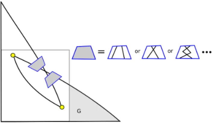
Let us go back to the argument. By symmetry, we can restrict ourselves to the case when V and W both lie in the positive sector. Let M and
∂M respectively denote the set of small and perfect vectors. We show that
E(∂M) is contained in a subset ∂N ⊂ ΠZ. The boundary of ∂N, which we
denote by ∂0N, is the graph of a smooth function in polar coordinates. The
yellow region in Figure 3.1 shows part of the portion of ∂N that lies in the positive sector. See Figure 5.1 for an expanded view. There 3 symmetrically placed components in the other sectors which we are not showing.
Figure 3.1: ∂0N+ (black), ∂N+ (yellow), ΛL (blue), and ∆L (red).
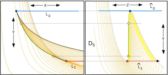
If we suppose that W is small and E(W) = E(V) then the flowline corresponding to W must be small symmetric. We can arrange all the small symmetric flowlines in a given loop level set into two curves. One of the curves corresponds to small symmetric flowlines whose initial endpoint has positive Z-coordinate. Given the loop level set of period L in the positive sector, we let ΛL denote the image, under E, of the corresponding vectors.
The blue curves in Figure 3.1 show ΛL for various choices of L.
On the right side of Figure 3.1 we focus on Λ5. We also draw the right
triangle ∆5 whose endpoints are the endpoints of Λ5. We define the triangle
∆Lfor other values ofLin the same way. In [CS,§3] we prove that ΛL⊂∆L
and that the interior of ΛL lies in the interior of ∆L. Finally, we show that
∂0N intersects ∆L only at the top vertex. These ingredients combine to show
4.3
The Differential Equation
We will now go into more detail about how the Bounding Triangle Theorem is proved. Let ℓ=L/2. We consider the backwards flow along the structure field Σ, namely
x′
=−xz, y′
= +yz, z′
=x2 −y2, (19) with initial conditions x(0)> y(0)>0 andz(0) = 0 chosen so that the point is in the loop level set of period L. (We will often denote these functions as xL, etc.) We let gt be the small symmetric flowline whose endpoints are
(x(t), y(t), z(t)) and (x(t), y(t),−z(t)). Then
ΛL(t) = (a(t), b(t),0) = Λgt.
Taking the derivative, we have (a′ , b′ ,0) = Λ′ L(t) = limǫ→0 ΛL(t+ǫ)−Λ(t) ǫ , ΛL(t+ǫ)≈(ǫx, ǫy, ǫz)∗(a, b,0)∗(ǫx, ǫy,−ǫz).
The approximation is true up to order ǫ2 and (∗) denotes multiplication in
Sol. A direct calculation gives
a′
= 2x+az, b′
= 2y−bz. (20) The initial conditions are a(0) = b(0) = 0. (We will often denote these functions as aL and bL.
Lemma 4.1 For any r≥0 we have
a(r)x(r) = Z r 0 2x2dt, b(r)y(r) = Z r 0 2y2dt. Proof: We have (ax)′ = 2x2 and (by)′ = 2y2. Alsoa(0) =b(0) = 0. Now we simply integrate. ♠ Lemma 4.2 b(0) a(0) = b(ℓ) a(ℓ). (21)
Proof: This comes from L’hopital’s rule and the Reciprocity Lemma. Let us take the opportunity to give a swift proof here. (This is another proof of the Reciprocity Lemma in a special case.) By two applications of Lemma 4.1, we have a(ℓ)x(ℓ) = Z ℓ 0 2x2 dt, b(ℓ)y(ℓ) = Z ℓ 0 2y2 dt.
But these two integrals are equal, by symmetry. Hence a(ℓ)x(ℓ) =b(ℓ)y(ℓ). Finally, we have x(0) =y(ℓ) andy(0) =x(ℓ) by symmetry. Combining these equations gives the result. ♠
The function b(t)/a(t) has the same value at t = 0 and t = ℓ. To finish the proof, we just have to show thatb(t)/a(t) cannot have a local maximum. This boils down to the fact that ab′′
−ba′′
= 2ab(y2−x2), a quantity which
is negative for t < ℓ/2 and positive for t > ℓ/2. These properties, together with the fact that a′
5
More Information about the ODE
In this chapter we further explore the ODE we introduced in the previous chapter. The results here do not appear in [CS]. However, they are rather similar in spirit to some of the results there. Lemma 4.1 above has a lot of juice in it, and we want to squeeze some more out. The estimates here will be useful when we consider the projections of the Sol spheres into the Euclidean plane ΠZ.
5.1
Bounding the Coordinates
In the next lemma, 2∗refers to a number which we can make as close as we like to 2 by taking Lsufficiently large. This result says that the boundary of the yellow region in Figure 3.1 asymptotes to the lines X = 2 andY = 2.
Lemma 5.1 b(ℓ)<2∗
.
Proof: From Lemma 4.1 and symmetry we have
y(ℓ)b(ℓ) = Z ℓ 0 y2 = Z ℓ/2 0 (x2+y2)dt.
The last equality follows from the fact that the function t→x2(t) +y2(t) is
periodic with period ℓ/2. Since b(ℓ)∼1 for largeL, it suffices to prove that the integral on the right approaches 1 as L→ ∞.
We have Z ℓ/2 0 (x2+y2)dt= Z ℓ/2 0 (x2−y2)dt+ 2 Z ℓ/2 0 y2dt. (22)
Now observe that Z ℓ/2 0 (x2−y2)dt= Z ℓ/2 0 z′ dt=z(ℓ/2)−z(0) =z(ℓ/2)∼1. (23)
To finish the proof, it suffices to show that Z ℓ/2
0
Let α be such that (x(0), y(0),0) lies in the same loop level set as (α, α,√1−2α2).
Then y ≤ α on [0, ℓ/2] because y is monotone increasing on this interval. Hence, by Equation 12 and some algebraic manipulation,
Z ℓ/2 0 y2dt≤Lα×α2 = 2α r 4α2 1 + 2α2 × K 1−2α2 1 + 2α2 . Setting m= 1−2α2 1+2α2, we see that Z ℓ/2 0 y2dt≤2α√1−m× K(m). (25)
As L→ ∞ we have α→0 and m→1 and K(m)∼ −log(1−m)/2. Hence, the right hand side of Equation 25 tends to 0 as L→ ∞. ♠
Remark: We also have a(ℓ)b(ℓ)∼eℓ, as discussed in [CS, §3.7] and also on
[G, p 75]. Lemma 5.2 a(L) = 2b(ℓ). Proof: We have a(L)x(L) = Z L 0 2x2dt= Z ℓ 0 2x2dt+ Z L ℓ 2x2dt= 2 Z ℓ 0 2y2dt= 2b(ℓ)y(ℓ). Hence a(L)x(L) = 2b(ℓ)y(ℓ).
But x(L) =y(ℓ), so we can cancel these terms to get the desired equality. ♠
5.2
The Doubling Lemma
It will be useful for us to consider flowlines which end on the plane Z = 0. These are the initial halves of symmetric flowlines. Here doubling refers to comparing the first half of a symmetric flowline with the whole thing.
Letgtdenote the first half of the flowlinegt; it connects the initial point of
gt to the midpoint of gt. Say that the coordinates of Λgt are (a(t), b(t), c(t)).
The coordinate c(t) is typically nonzero, but we do not care about it. Define ΛL(t) = (aL(t), bL(t))⊂R2. (26)
In the next lemma we identity ΠZ withR2.
Lemma 5.3 (Doubling) Λ(t) = 1 2ΛL(t). Proof: We have (a′, b′, c′) = lim ǫ→0 ΛL(t+ǫ)−Λ(t) ǫ , ΛL(t+ǫ)≈(ǫx, ǫy, ǫz)∗(a, b, c).
Taking the limit, we find that
a′
=z+ax, b′
=z−bx. (27) (Also c′
=z. We have the same initial conditions a(0) =b(0) as above. Now notice that this solution to this equation is given by a=a/2 and b=b/2. ♠
Corollary 5.4 b(ℓ) =a(L).
Proof: We combine the Doubling Lemma and Lemma 5.2 to get the
equa-tion b(ℓ) =a(L)/2 =a(L). ♠
Now we give some applications, which show how the Doubling Lemma and our asymptotics above give us some specific information about some geodesic segments in Sol. Let f(r, L) denote the flowline of length r on the loop level set of period L which ends at the point (x, y,0) with x > y. Let
Υr(L) = Λf(r,L).
This is the endpoint of the corresponding geodesic segment. The isochronal curve L→Υr(L), forL∈[r,∞) will be a central object later in the paper.
1. We have Υr(r) ∼ (2, er/2/2,0) by Lemma 5.1 and the remark after
2. We have Υr(2r)∼(er/4,1,∗) by Case 1, and symmetry, and the
Dou-bling Lemma.
3. We have Υr(4r)∼(er/2,∗,∗).
We do not need Item 3 for any purpose, so we will be a bit sketchy with the proof. The small symmetric flowline of which f(r,4r) is the first half starts at (0,0, z) and ends at (0,0,−z) for the appropriate choice of z. The corresponding geodesic segment γ of length 2r connects the origin to a point in ΠZ and remains nearly tangent to ΠY. Also, γ starts and ends nearly
vertically. In fact, γ is asymptotic to the geodesic segment considered in Lemma 2.1. Thus, the first coordinate of the far endpoint of γ is asymptotic to er. By the Doubling Lemma, the first coordinate of Υ
r(4r) is asymptotic
to er/2.
For what it is worth, the second coordinate tends to 0 asr→ ∞. To see this, note that the product of the first two coordinates of γ is, by Lemma 4.1, 4 x(r)y(r) Z r 0 x2dt Z r 0 y2dt∼ 4 x(r)y(r) Z r 0 y2dt < 4ry(r) 2 x(r)y(r) = 4r.
The asymptotic estimate ∼ is Equations 23 – 24. The last inequality comes from the monotone increasing nature ofy(t) fort∈[0, r]. The equality comes from the fact that x(r) =y(r).
6
The Euclidean Projection
6.1
Notation
We introduce some notation that we use through out the chapter. We will consider some quantity F that depends on the variable r or the variable L. The statement F < ζ∗
means that, for any ζ∗
> ζ we can make F < ζ∗ provided that we take r orL sufficiently large.
6.2
The Cut Locus Image
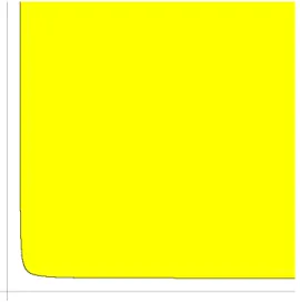
Figure 6.1 shows a more of the yellow region in Figure 3.1. In this section we will prove a result which is equivalent to the statement that the horizontal asymptote of the boundary curve is the line y = 2. Similarly, the vertical asymptote is the line x= 2.
Figure 6.1: ∂N in the positive quadrant.
Say that a vector is positive if all its coordinates are positive. Say that a vector is distinguished if its corresponding flowline is contained in a small symmetric flowline with the same initial point. That is, the flowline cor-responding to the distinguished vector can be prolonged until it is a small symmetric flowline. In particular, distinguished vectors are small.
Theorem 6.1 (Asymptotic) If V is a distinguished positive vector whose
corresponding flowline is contained in a loop level set of period L, then
E(V) = (a, b,0) has the property that b∈(0,2∗ ).
Proof: First consider the special case when V corresponds to a small sym-metric flowline. Then b = bL(t) for some t ≤ ℓ. By the Bounding Triangle
Theorem and Lemma 5.1, bL(t)≤bL(ℓ)<2∗.
Now consider the case when V is an arbitrary distinguished positive vec-tor. There is some λ ≥ 1 so that λV corresponds to a small symmetric flowline. The X and Y coordinates of the curve t → E(tV) are increasing functions because it is impossible for the geodesic associated to V to be tan-gent to the hyperbolic foliations of Sol. (Otherwise this geodesic would be trapped inside a leaf of the foliation for all time.) In particular, the second coordinate ofE(V) is less or equal to the second coordinate ofE(λV), which is in turn less than 2∗
by the special case. ♠
6.3
The Area Bound
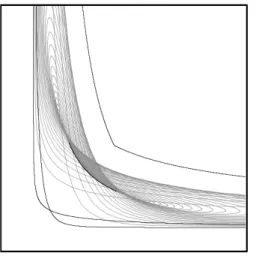
Our main goal is to show thatAZ(Sr)<16∗er. Lemma 6.2 below is the main
ingredient in the proof. This result says that when (a, b) ∈ ηZ(Sr) we have
min(a2b, ab2) < 2∗
er. Figure 6.2 indicates the plausibility of this estimate.
Figure 6.2 shows the projection of (part of the positive sector of) S5 into
the plane ΠZ. The small black arc of a hyperbola is the projection of the
singular set. The outer black curve is min(xy2, x2y) =e5.
Figure 6.2: Projection into the plane ηZ.
Lemma 6.2 Let (a, b, c) = E(V), where V is a small or perfect vector of
length r. Then min(ab2, a2b)<2∗
er and max(a, b)<(1/2)∗
Proof: Note that as r → ∞, the period of the loop level set containing V
also tends to ∞. This makes the Asymptotic Lemma available to us.
Letγ be the geodesic segment corresponding toV. Let g be the flowline corresponding to V. We can write g =g1|g2 where one of two things is true:
• g1 is distinguished and g2 is empty.
• g1 is small symmetric and g2 is distinguished.
After interchanging the roles of X and Y if necessary, we reduce to 2 cases.
Case 1: Let γ1 be the geodesic segment corresponding to g1, having
end-point (a, b, c). By the hyperbolic estimates, we know that ηY(γ1) lies in the
hyperbolic disk Dr in ΠY centered at the origin. By Lemma 2.2, we have
a < (1/2)∗
er. We also have b < 2∗
by the Asymptotic Theorem. Hence
ab2 <2∗
er. We also see that max(a, b)<(1/2)∗
er.
Case 2: Let γ1 and γ2 repectively be the geodesic segments
correspond-ing to g1 and g2. Let rj be the length ofγj. Let (aj, bj) be the projection to
ηZ of the far endpoint of γj.
Let γ′
1 be the geodesic segment which is the first half of γ1, in terms of
length. So, γ′
1 and γ1 have the same initial endpoint (the origin) butγ1′ has
lengthr1/2. Let (a′1, b
′
1) be the far endpoint ofηZ(γ1′). Onceris large enough
we have the following:
• By Lemma 2.1, a1 ≤er1/2−e−r1/2.
• By the Asymptotic Theorem, b1 <2∗.
• By Lemma 2.2 and symmetry, b2 ≤(er2 −e−r2)/2.
• By symmetry and the Asymptotic Theorem, a2 <2∗.
Combining these observations, we have
a ≤2∗ +er1/2 −e−r1/2, b ≤2∗ + (er2 −e−r2)/2. (28)
We have r1+r2 =r. We get right away that max(a, b)<(1/2)∗er.
Now we consider a2b. Suppose first that both r
1 and r2 tend to ∞. In
this case a <1∗
When r1 is bounded andr2 → ∞, a2b < (1/2)∗ a2er2 =er × 1 2 + e−2r1 2 −2e −3r1/2 +e−r1 + 2e−r1/2 <2∗ er.
The last inequality follows from a bit of calculus.
When r2 is bounded andr1 → ∞ we have a <1∗e(r−r2)/2. This gives
a2b <1∗ er× 1−e−2r2 + 2e2r2 <2∗ er.
This completes the proof. ♠
Once r is sufficiently large, the sphere S′
r consists entirely of small and
perfect vectors either contained in the planes ΠX and ΠY or else lying in loop
level sets whose period is so large that Lemma 6.2 holds for them. Lemma 6.2 shows that the projection of the positive sector of Sr lies in the region
Ωr defined by the following inequalities.
X, Y ∈[0,(1/2)∗
er], min(xy2, yx2) = 2∗
er. (29) We set x0 = y0 = (2∗er)1/3. The region Ωr is the union of the square
[0, x0]×[0, y0], whose area is 0∗er, and two other regions which are swapped
by reflection in the main diagonal x = y. One region lies underneath the graph y = (2∗
er/x)1/2 starting at x = x
0 and ending at x= (1/2)∗er. This
region has area √ 2∗er/2 Z (1/2)∗ er x0 dx √ x < √ 2∗er/2 ×2×p(1/2)∗er <2∗ er, (30)
once r is large. Hence Ωr has area at most 4∗er. Recalling that Ωr contains
the projection of the positive sector of Sr, which is 1/4 of the whole sphere,
we see that AX(Sr)<16∗er.
Remark: The set ηX(Sr) contains the region Gr above the X-axis,
un-derneath the arc Υr[2r,4r] discussed in §5.2, and to the right of the line
x = e2 ×er/2. Given our Embedding Theorem below, and the estimates
in §5.2, we see that the upper boundary of Gr is the graph of a decreasing
function whose domain has length er/4∗
and whose minimum is asymptotic to 1. Thus Gr contains a rectangle of area e4/4∗. HenceAX(Sr)>(2/1∗)er.
6.4
The Yin Yang Curve
Given r, we define the yin-yang curve Yr to be the set of points in Sr′ where
the differential d(ηZ ◦E) is singular. For r ≤ π
√
2 the the curve Yr is
connected. For r > π√2, the curve has 2 disjoint components interchanged by the map (x, y, z)→(y, x,−z).
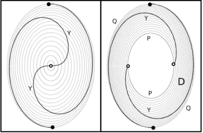
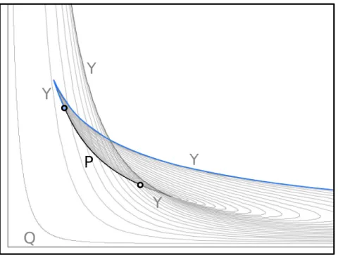
Figure 6.3: The yinyang curves for r=π√2 and r= 5.
Figure 6.3 shows the yin-yang curves for r = π√2 and for r = 5. In Figure 6.3, we are projecting the unit sphere in R3 onto the plane through
the origin perpendicular to the vector (1,−1,0). The loop level sets all project to ellipses having aspect ratio √2. On the right side of Figure 6.3, the ellipse labeled P is the set of perfect vectors on S′
5. The ellipse labeled
Q is the intersection of the positive sector of the unit sphere with the planes
X = 0 andY = 0. Notice thatPr∪Yr∪Qrdivides Sr′ into a union of 2 disks.
The mapηZ◦Π is nonsingular on the interior of these disks and hence a local
diffeomorphism. This is what is important for our Projection Estimate 4. Referring to Figure 6.3, the union Yr ∪Pr ∪Qr separates the positive
sector of S′
r into 2 components. The map (x, y, z)→(x, y,−z) interchanges
these components. Let Dr be either of these disks. Below, we will describe
more clearly which of the two choices we take to be Dr. Figure 6.4 shows
Figure 6.4: The image ηZ◦E(D5).
The region labeled Y in Figure 6.3 is the image ηZ ◦E(Yr). We define
Υr = ηZ ◦E(Yr∗), where Y
∗
is the component of Yr whose endpoint in ΠX
is a point of the form (xr, yr,0) with xr > yr. We have drawn Υr in blue in
Figure 6.4.
The mapL→Υr(L) is a smooth, and indeed real analytic, map. We say
that a cusp of this map is a point where the map is not regular. So, away from the cusps, Υr is a smooth regular curve. Figure 6.3 suggests that Υ5
just has a single cusp. We prove the following result in the next chapter.
Theorem 6.3 (Embedding) For r sufficiently large, the curve Υr has a
single cusp, and negative slope away from a single cusp. The cusp κr =
(ar, br, cr) satisfies the bounds ar <2∗ and br <(e2/2)∗er/2.
6.5
The Multiplicity Bound
The image ηZ◦E(∂Dr) is a piecewise analytic loop. We will show that this
loop winds at most twice around any point in the plane that it does not contain. Referring to §2.3, we apply the Disk Lemma to h = ηZ ◦E and
at most 4-to-1 on the positive sector of S′
r. HenceηZ is at most 4-to-1 on the
positive sector of Sr. Since the different sectors project into ηZ disjointly,
we see that ηZ is at most 4-to-1 on all of Sr. This establishes our estimate
NZ(Sr) = 4.
Now we turn to the analysis of the imageηZ◦E(∂Dr). Define
Φr=E◦ηZ(Pr). (31)
Also, let R(x, y, z) = (y, x,−z). The image ηZ ◦E(∂Dr) is invariant under
R. It is the union of 5 analytic arcs:
• An arc of the X-axis connecting the origin to the endpoint of Υr.
• Υr.
• Φr.
• R(Υr).
• An arc of the Y-axis connecting an endpoint of R(Υr) to the origin.
Note that Υr∪Φr∪R(Υr) is a piecewise analytic arc that has its endpoints
in the coordinate axes and otherwise lies in the positive quadrant. The Embedding Theorem says that Υr has negative slope, and is smooth and
regular away from a single cusp. By symmetry, the Embedding Theorem also applies to R(Υr).
The cusps serve as natural vertices for our loop, so we make some new definitions which take the cusps into account. Let Φ∗
r denote the portion of
Υr∪Φr ∪R(Υr) that lies between the two cusps. Let Υ∗r = Υr −Φ∗r. The
loop ηZ◦E(∂Dr) has the same 5-part description as above, with Υ∗r and Φ
∗
r
used in place of Υr and Φr.
We will prove below that Υ∗
r∪Φ ∗ r is embedded. By symmetry, Φ ∗ r∪R(Υ ∗ r)
is also embedded. We will also prove that Υ∗
r crosses the main diagonal – the
fixed point set of R – exactly once. This information forces the schematic picture of ηZ ◦E(∂Dr) shown in Figure 6.5.
or or
Figure 6.5: Schematic picture of ηZ◦E(D5).
Numerically, it seems that the first option occurs, and that the two curves Υ∗
r and R(Υ
∗
r) intersect exactly once. We did not want to take the trouble to
establish this fact, given the already lengthy nature of the paper. In any case, the information above establishes the fact that ηZ ◦E(∂Dr) winds at most
twice around any point in the plane that does not lie in its image. Applying the Disk Lemma to the map h=ηZ◦E and the disk Dr we see that h is at
most 2-to-1 on Dr. But then h is at most 4-to-1 onDr∪I(Rr) =Sr++. This
completes the proof of Projection Estimate 4, modulo the properties of Υ∗
r
and Φ∗
r. We now turn to the task of establishing the properties about the
topology of this planar loop.
Now we turn to the proof of Projection Estimate 5. It follows from the negative slope of Υr and R(Υr) that any intersection between these two
curves lies in the square whose opposite corners are the two cusps. What we mean is that all the “tangles” shown in Figure 6.5 lie inside the lightly shaded square. Hence, h is injective on the portion of Dr which maps outside this
square. Referring to the Embedding Theorem, the shaded square is bounded by the lines x = br and y = br, where we know that br < (e2/2)er/2. The
same analysis as done in connection with Equation 30 shows that
Ar,3+Ar,4 < K1e2r/3 + 2Ir, where Ir = √ 2∗er/2 Z (e2/2)∗er/2 x0 dx √ x < K2e 3r/4. (32)
6.6
The Topology of the Boundary
Lemma 6.4 For r sufficiently large, the curve Υ∗
r∪Φ
∗
r is embedded.
Proof: Our argument refers to Figure 6.6. Let γ be the portion of Υ∗
r∪Φ
∗
r
that lies above the (red) horizontal line L1 through the cusp of R(Υ∗r). This
point is the endpoint of Φ∗
L.
Figure 6.6: Projections of the relevant sets.
By the Embedding Theorem, γ has a single cusp, namely the cusp of Υr.
Let γ1 and γ2 be the two arcs ofγ on either side of this arc. These two arcs
have negative slope and no cusps on them. Hence all of γ lies between the horizontal lineL0 through the cusp of Υr and the horizontal line through the
cusp of R(Υr). These are the red and yellow horizontal lines on the left side
of Figure 6.6.
Sinceγ1andγ2have negative slope and no cusps, they are each embedded.
We just have to see that γ1 cannot intersect γ2. We will suppose that there
is an intersection and derive a contradiction.
The portion of the Sol sphereSr lying in the positive sector is the union
of two disks,Dr andR(Dr), whereR is the isometry extending our reflection
in the main diagonal of ΠZ, namely I(x, y, z) = (y, x,−z). The common
boundary of these disks contains a curve bγ which projects to γ. We have b
γ = bγ1∪bγ2. On the right side of Figure 6.6, one of these arcs connects the
to the red vertex. The right side of Figure 6.6 shows the projection into the
Y Z plane.
Because no plane tangent toSr at an interior point of bγ is vertical, each
plane of the form Y = const. intersects each of bγ1 and bγ2 exactly once. In
particular, this is true to the planes Lb0 and Lb1 which respectively project to
L0 and L1 on the left side of Figure 6.6.
One of the two disks Dr or R(Dr) has the property that it lies locally
One of the two disks – say Dr – lies between Lb0 and Lb1 in a neighborhood
of bγ. We are taking about the yellow highlighted region on the right side of Figure 6.6. The interior of Dr is transverse to the plane Lb1 because ηZ is
a local diffeomorphism on the interior of Dr. But this means that Dr ∩Lb1
contains a smooth arc βbwhich connects the endpoint of γ1 to the endpoint
of γ2. Let β=ηZ(βb). We note the following
• β is contained in the line L1.
• The endpoints of β coincide.
• The interior of β is a regular curve.
These properties are contradictory, because β would have to turn around in
L1at an interior point, violating the regularity. This contradiction establishes
the result that γ is embedded.
It remains to consider the portion of Υr ∪ Φr ∪ R(Υ∗r) that lies
be-low the horizontal line L1 through the cusp of R(Υ∗r). We label so that
Φr∪R(Υ∗r) ⊂γ2. Given that γ2 has negative slope we see that Φr∪R(Υ∗r)
lies entirely aboveL1. But this means that the portion ofγ1 belowL1 is
dis-joint from γ2. Finally, the portion ofγ1 belowL1 is disjoint from the portion
of γ1 above L1 because γ1 is regular and has negative slope. ♠
Define
Υ∗∗
r = Υr[r,2r]−Υ
∗
r. (33)
This is the subset of Υr[r,2r] that occurs after the cusp. Given our result
above, the only self-intersections on the curve ηZ◦D(∂Dr) occur where Υ∗∗r
andR(Υ∗∗
r ). These are analytic arcs of negative slope, and they are permuted
by the map R. Hence, the can only intersect finitely many times, and their intersection pattern must be as in Figure 6.6. This completes the proof of Projection Estimate 4, and hence the Volume Entropy Theorem, modulo the proof of the Embedding Theorem.
7
The Embedding Theorem
7.1
The Isochronal Curves
Let ΛL = (aL, bL), as in §4.3. Let E be the Riemannian exponential map and letηZ be projection into the plane ΠZ. We have Υr =ηZ◦E(Yr∗), where
Y∗
r is the relevant component of Yr.
Lemma 7.1 Υr(L) = ΛL(r).
Proof: Recall that S′
r is the set of perfect vectors of length r contained in
the positive sector of R3. Define the positive side of S′
r ∩ΠZ to be those
vectors of the form (x, y,0) with x > y >0. By definition, Υr(L) =ηZ ◦E(Y
∗
r), (34)
where Y∗
r is the component of the yin yang curve Yr which ends in the
positive side. The vectors V ∈Yr are characterized by the property that the
differential d(ηZ◦E) is singular at points of Yr.
The kernel of the projection map ηZ is spanned by the vector (0,0,1).
So, the differential d(ηZ ◦E) is singular at V if and only if dE maps the
tangent plane to S′
r at V to a plane which contains the vector (1,0,0). But
then dE(NV) is orthogonal to (0,0,1). Here NV is normal to Sr′ at V. But
this means that the third coordinate of dE(NV) is 0. Given the connection
between the Haniltonian flow onS′
rand the geodesics, this situation happens
if and only if the flowline associated to V ends in the plane ΠZ.
In short, Yr consists of those small or perfect vectors of length r whose
corresponding flowlines end in ΠZ. But these flowlines are then the initial
halves of symmetric flowlines which wind at most twice around their loop level sets. The points in Y∗
r are the initial halves of symmetric flowlines
whose midpoints lie on the positive side of S′
r. Moreover, these symmetric
flowlines wind at most twice around their loop level sets and every amount of winding, so to speak, from 0 times to 2 times, is achieved. So, by definition Υr = Λ(r). ♠
We call Υr an isochronal curve because it computes all the solutions to
the differential equation at the fixed time r. Figure 7.1 shows part of Υ5.
Figure 7.1: The ΛL curves and the initial part of Υ5.
7.2
The Tail End
Lemma 7.2 The curve Υr(2r,∞) is smooth, regular, and embedded.
Proof: The flowline corresponding to the point Υr(L) lies on the loop level
set of period L and flows for time r. If L >2r then the flowline travels less than halfway around the loop level set. Thus, the flowline is the initial half of a small symmetric arc. Let S ⊂R3 denote the set of vectors corresponding
to small symmetric flowlines. The map E is a diffeomorphism on S, because
S consists entirely of small vectors. This is part of the Cut Locus Theorem from [CS]. By the Doubling Lemma,
Υr(2r,∞) =
1
2E(Cr),
whereCr ⊂Sis a smooth regular curve, obtained by dilating a suitably
cho-sen arc of the yin yang curve by a factor of 2. Since E is a diffeomorphism on S, we see that 1
7.3
The Slope
Let xL, etc. be the functions described at the end of §4.3. These functions
satisfy the ODE
x′
=−xz, y′
=yz, z′
=x2−y2, a′
=x+az, b′ =y−bz, (35) with initial conditions
xL(0)> yL(0) > zL(0) =aL(0) =bL(0) = 0, (xL(0), yL(0),0)∈ΘL. (36)
Here ΘL is the loop level set, in the positive sector, having period L. I am
grateful to Matei Coiculescu for help with the following derivation.
Lemma 7.3 Υr has negative slope away from the cusps.
Proof: This proof is a calculation with the ODE. For any relevant function
f, the notation ˙f means∂f /∂L. We compute ( ˙a)′ = ∂ ∂L ∂a ∂t = ∂ ∂L(x+za) = ˙x+ ˙az+ ˙za.
By the product rule (xa˙)′
=x′ ˙
a+x( ˙a)′
=−zxa˙ +xz˙+xza˙ +axz˙ =xx˙+axz.˙ This calculation, and a similar one, show that
(xa˙)′
=xx˙ +axz,˙ (yb˙)′
=yy˙−byz˙ (37) Since x2 +y2+z2 ≡1 we have xx˙ +yy˙+zz˙ = 0. Adding the Equations in
Equation 7.3 and using this relation, we find that.
(xa˙ +yb˙)′ =xx˙ +yy˙+ (ax−by) ˙z =xx˙+yy˙+zz˙ = 0.
Hence xa˙+yb˙ is a constant function. Since a(0) =b(0) = 0 for allLwe have ˙
a(0) = 0 and ˙b(0) = 0. So, the constant in question is 0. Therefore
xa˙ +yb˙ = 0 (38) Because Υr(L) = ΛL(r), the velocity of Υr atL is
( ˙aL(r),b˙L(r)).
The slope of Υr at L equals −xL(r)/yL(r) by Equation 38, provided that
the velocity is nonzero. Since x, y are everywhere positive, the slope of Υr is
7.4
The End of Proof
In the next chapter we prove the following result.
Lemma 7.4 (Monotonicity) If L is sufficiently large then there is some
tL∈(L−1, L) such that the functionb˙L is negative on [L/2, tL) and positive
on (tL, L]. Moreover, the function L→tL is monotone increasing.
Corollary 7.5 Υr[r,2r] has exactly one cusp.
Proof: The curve Υr has a cusp at Lif and only if its velocity
( ˙aL(r),b˙L(r))
vanishes. By Lemma 38, one coordinate of the velocity vanishes if and only if the other one does. So, Υr has a cusp atL if and only if ˙bL(r) = 0. Suppose
then that Υr[r,2r] has more than one cusp. Then there are at least two pairs
(r, L1) and (r, L2) such that ˙bL1(r) = 0 and ˙bL2(r) = 0. This means that
r =tL1 =tL2. But this contradicts the Monotonicity Lemma. Hence Υr has
at most one cusp.
Since the map L → tL is unbounded, each sufficiently large r lies in its
image. But this means that for sufficiently largerthere is someL∈(r, r+ 1) such that r = tL. This means that Υr has a cusp at L. Hence, once r is
sufficiently large, Υr has exactly one cusp. ♠
This completes the proof of the Embedding Theorem, but there is one more remark we want to make. The cusp of Υr occurs at some L∈(r, r+ 1).
This explains why, in Figure 7.1, the cusp appears all the way to the left, near the end of Υ5.
The next two chapters are devoted to the proof of the Monotonicity Lemma.
8
The Vanishing Point
8.1
Auxiliary Functions
In this chapter we will prove the first half of the Monotonicity Lemma. That is, we will show that onceLis sufficiently large there is a pointtL∈[L−1, L]
such ˙bL vanishes at t0, and this is the only vanishing point. We sometimes
set ˙f =∂f /∂Land f′
=∂f /∂t. We introduce the following functions.
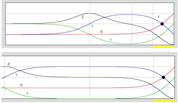
Z = ˙z, X = ˙x/x, Y = ˙y/y, B = ˙b/b, (39) Sincea, b, x, y >0 these functions respectively have the same signs as ˙z,x,˙ y,˙ b˙.
Figure 8.1: Numerical plots
The top half of Figure 8.1 shows numerical plots of these functions at
L = 8. The bounding box in the picture is [0,8]×[−1,1]. The bottom half shows the plot of the functions at the value L = 16. This time we are just showing the right half of the plot. Notice that in the interval [L−1, L] the plots line up very nicely. The black dot in both cases is the point (tL,0).
One half of the Monotonicity Lemma establishes thattL is uniquely defined.
The second half shows thattLincreases monotonically. The intuition behind
the second half of the result is that the pictures in [L−1, L] stabilize, so that
8.2
Differentiation Formulas
In this section we derive the following formulas. 1. X′ =−Z 2. Y′ = +Z 3. Z′ =−4y2Y −2zZ. 4. B′ = yb(Y −B)−Z. 5. Z′′ = (−2 + 6z2)Z.
(1) From the relation x′
=−xz we get ( ˙x)′ =−xz˙ −zx˙ . Then we get: X′ = ˙ x x ′ = −xz˙ −zx˙ x − ˙ xx′ x2 =−z˙− ˙ xz x + ˙ xz x =−z˙ =−Z
(2) From the relation y′
=yz we get ( ˙y)′ = ˙yz+ ˙zy. Then we get: Y′ = ˙ y y ′ = yz˙ + ˙zy y − ˙ yy′ y2 = ˙z+ ˙ yz y − ˙ yz y = ˙z =Z
(3) From the relations z′
=x2−y2 and x2 = 1−y2−z2 we get
Z′
= 2xx˙ + 2yy˙ = 2x2X−2y2Y, 2x2X =−2y2Y −2zZ.
Substitute the second relation into the first to get the formula above.
(4) Note that ˙b/b = ˙b/b because b = b/2. So, we work with b for ease of notation. From the relation b′
= 2y−bz we get (˙b)′ = 2 ˙y−zb˙ −zb˙ . Then: B′ = ˙ b b ′ = 2 ˙y−zb˙ −bz˙ b − ˙ bb′ b2 = 2 ˙y−zb˙ −bz˙ b − 2˙by−bbz˙ b2 = 2 ˙y b − 2˙by b2 −z˙= 2y b (Y −B)−Z = y b(Y −B)−Z.
(5) We first work out that
z′′ =−2z+ 2z3. (40) We then compute Z′′ = ∂z ′′ ∂L = ∂(−2z+ 2z3) ∂L = (−2 + 6z 2)Z.