ERIMREPORT SERIES RESEARCH IN MANAGEMENT
ERIM Report Series reference number ERS-2009-001-LIS
Publication January 2009
Number of pages 42
Persistent paper URL http://hdl.handle.net/1765/14528 Email address corresponding author [email protected]
Address Erasmus Research Institute of Management (ERIM) RSM Erasmus University / Erasmus School of Economics Erasmus Universiteit Rotterdam
P.O.Box 1738
3000 DR Rotterdam, The Netherlands Phone: + 31 10 408 1182 Fax: + 31 10 408 9640 Email: [email protected] Internet: www.erim.eur.nl
Bibliographic data and classifications of all the ERIM reports are also available on the ERIM website: www.erim.eur.nl
How to Normalize Co-Occurrence Data? An Analysis of
Some Well-Known Similarity Measures
E
RASMUS
R
ESEARCH
I
NSTITUTE OF
M
ANAGEMENT
REPORT SERIES
RESEARCH IN MANAGEMENT
A
BSTRACT ANDK
EYWORDSAbstract In scientometric research, the use of co-occurrence data is very common. In many cases, a similarity measure is employed to normalize the data. However, there is no consensus among researchers on which similarity measure is most appropriate for normalization purposes. In this paper, we theoretically analyze the properties of similarity measures for co-occurrence data, focusing in particular on four well-known measures: the association strength, the cosine, the inclusion index, and the Jaccard index. We also study the behavior of these measures empirically. Our analysis reveals that there exist two fundamentally different types of similarity measures, namely set-theoretic measures and probabilistic measures. The association strength is a probabilistic measure, while the cosine, the inclusion index, and the Jaccard index are set-theoretic measures. Both our set-theoretical and our empirical results indicate that co-occurrence data can best be normalized using a probabilistic measure. This provides strong support for the use of the association strength in scientometric research.
Free Keywords similarity measure, association strength, cosine, inclusion index, Jaccard index Availability The ERIM Report Series is distributed through the following platforms:
Academic Repository at Erasmus University (DEAR), DEAR ERIM Series Portal
Social Science Research Network (SSRN), SSRN ERIM Series Webpage
Research Papers in Economics (REPEC), REPEC ERIM Series Webpage
Classifications The electronic versions of the papers in the ERIM report Series contain bibliographic metadata by the following classification systems:
Library of Congress Classification, (LCC) LCC Webpage
Journal of Economic Literature, (JEL), JEL Webpage
ACM Computing Classification System CCS Webpage
How to normalize co-occurrence data?
An analysis of some well-known similarity measures
Nees Jan van Eck
∗†Ludo Waltman
∗∗
Econometric Institute, Erasmus School of Economics
Erasmus University Rotterdam
P.O. Box 1738, 3000 DR Rotterdam, The Netherlands
E-mail:
{nvaneck,lwaltman}@ese.eur.nl
†
Centre for Science and Technology Studies, Leiden University
P.O. Box 905, 2300 AX Leiden, The Netherlands
Abstract
In scientometric research, the use of co-occurrence data is very common. In many cases, a similarity measure is employed to normalize the data. However, there is no consen-sus among researchers on which similarity measure is most appropriate for normalization purposes. In this paper, we theoretically analyze the properties of similarity measures for co-occurrence data, focusing in particular on four well-known measures: the association strength, the cosine, the inclusion index, and the Jaccard index. We also study the behav-ior of these measures empirically. Our analysis reveals that there exist two fundamentally different types of similarity measures, namely set-theoretic measures and probabilistic mea-sures. The association strength is a probabilistic measure, while the cosine, the inclusion index, and the Jaccard index are set-theoretic measures. Both our theoretical and our em-pirical results indicate that co-occurrence data can best be normalized using a probabilistic measure. This provides strong support for the use of the association strength in scientomet-ric research.
Keywords
1 Introduction
The use of co-occurrence data is very common in scientometric research. Co-occurrence data can be used for a multitude of purposes. Co-citation data, for example, can be used to study relations among authors or journals, co-authorship data can be used to study scientific cooper-ation, and data on co-occurrences of words can be used to construct so-called co-word maps, which are maps that provide a visual representation of the structure of a scientific field. Usually, when co-occurrence data is used, a transformation is first applied to the data. The aim of such a transformation is to derive similarities from the data or, more specifically, to normalize the data. For example, when researchers study relations among authors based on co-citation data, they typically derive similarities from the data and then analyze these similarities using multivariate analysis techniques such as multidimensional scaling and hierarchical clustering (e.g., McCain, 1990; White and Griffith, 1981; White and McCain, 1998). Likewise, when researchers use co-authorship data to study scientific cooperation, they typically apply a normalization to the data and then base their analysis on the normalized data (e.g., Gl¨anzel, 2001; Luukkonen, Persson, and Sivertsen, 1992; Luukkonen, Tijssen, Persson, and Sivertsen, 1993).
In this paper, our focus is methodological. We study various measures for deriving similar-ities from co-occurrence data. Basically, there are two approaches that can be taken to derive similarities from co-occurrence data. We refer to these approaches as the direct and the indi-rect approach, but the approaches are also known as the local and the global approach (Ahlgren, Jarneving, and Rousseau, 2003; Jarneving, 2008). Similarity measures that implement the direct approach are referred to as direct similarity measures in this paper, while similarity measures that implement the indirect approach are referred to as indirect similarity measures.
The indirect approach to derive similarities from co-occurrence data relies on co-occurrence profiles. The occurrence profile of an object is a vector that contains the number of co-occurrences of the object with each other object. Indirect similarity measures determine the similarity between two objects by comparing the co-occurrence profiles of the objects. The indirect approach is mainly used for co-citation data (e.g., McCain, 1990, 1991; White and Griffith, 1981; White and McCain, 1998). From a theoretical point of view, the approach is quite well understood (Ahlgren et al., 2003; Van Eck and Waltman, 2008).
In this paper, we focus most of our attention on the direct approach to derive similarities from co-occurrence data. Direct similarity measures determine the similarity between two
ob-jects by taking the number of co-occurrences of the obob-jects and adjusting this number for the total number of occurrences or co-occurrences of each of the objects. Researchers use several different direct similarity measures. The cosine and the Jaccard index are especially popular, but other measures are also regularly used. However, relatively little is known about the the-oretical properties of the various measures. Also, there is no consensus among researchers on which measure is most appropriate for a particular purpose. In this paper, we theoretically an-alyze some well-known direct similarity measures and we compare their properties. We also study the behavior of the measures empirically. Usually, when a direct similarity measure is applied to co-occurrence data, the purpose is to normalize the data, that is, to correct the data for differences in the total number of occurrences or co-occurrences of objects. The main ques-tion that we try to answer in this paper is therefore as follows: Which direct similarity measures are appropriate for normalizing co-occurrence data and which are not? Interestingly, despite their popularity, the cosine and the Jaccard index turn out not to be appropriate measures for normalization purposes. We argue that an appropriate measure for normalizing co-occurrence data is the association strength (Van Eck and Waltman, 2007; Van Eck, Waltman, van den Berg, and Kaymak, 2006), also referred to as the proximity index (e.g., Peters and van Raan, 1993a; Rip and Courtial, 1984) or the probabilistic affinity index (e.g., Zitt, Bassecoulard, and Okubo, 2000). Although this measure is somewhat less well-known, it turns out to have the right theoretical properties for normalizing co-occurrence data.
This paper is organized as follows. We first provide an overview of the most popular direct similarity measures. We then analyze these measures theoretically. We also look for empirical relations among the measures. Finally, we answer the question which direct similarity measures are appropriate for normalizing co-occurrence data and which are not.
2 Overview of direct similarity measures
In this section, we provide an overview of the most popular direct similarity measures. The overview is based on a survey of the scientometric literature.
We first introduce some mathematical notation. LetO denote an occurrence matrix of or-der m×n. The columns of O correspond with the objects of which we want to analyze the co-occurrences. There aren such objects, denoted by 1, . . . , n. The objects can be, for
exam-ple, authors (e.g., White and McCain, 1998), countries (e.g., Gl¨anzel, 2001; Zitt et al., 2000), documents (e.g., Gm¨ur, 2003; Klavans and Boyack, 2006b), journals (e.g., Boyack, Klavans, and B¨orner, 2005; Klavans and Boyack, 2006a), Web pages (e.g., Vaughan, 2006; Vaughan and You, 2006), or words (e.g., Kopcsa and Schiebel, 1998). The rows of O usually correspond with documents.mthen denotes the number of documents on which the co-occurrence analysis is based. Sometimes the rows ofO do not correspond with documents. In Web co-link anal-ysis, for example, the rows of O correspond with Web pages (e.g., Vaughan, 2006; Vaughan and You, 2006). Throughout this paper, however, we assume for simplicity that the rows ofO
always correspond with documents. Another assumption that we make is that O is a binary matrix, that is, each element ofOequals either zero or one. Let oki denote the element in the
kth row andith column ofO. okiequals one if objectioccurs in the document that corresponds
with thekth row ofO, and it equals zero otherwise. LetCdenote the co-occurrence matrix of the objects1, . . . , n. Cis a symmetric non-negative matrix of ordern×n. Letcij denote the
element in theith row andjth column ofC. Fori6=j,cij equals the number of co-occurrences
of objectsiandj. Fori=j,cij equals the number of occurrences of objecti. Clearly, for alli
andj,cij =
Pm
k=1okiokj. It follows from this thatC=OTO, whereOT denotes the transpose
ofO. Moreover, the assumption thatOis a binary matrix implies thatCis an integer matrix. As we discussed in the introduction, there are two types of measures for determining simi-larities between objects based on co-occurrence data. We refer to these two types of measures as direct similarity measures and indirect similarity measures. Indirect similarity measures, also known as global similarity measures (Ahlgren et al., 2003; Jarneving, 2008), determine the similarity between two objects iand j by comparing the ith and the jth row (or column) of the co-occurrence matrixC. The more similar the co-occurrence profiles in these two rows (or columns) of C, the higher the similarity between iandj. Indirect similarity measures are especially popular for author co-citation analysis (e.g., McCain, 1990; White and Griffith, 1981; White and McCain, 1998) and journal co-citation analysis (e.g., McCain, 1991). We refer to Ahlgren et al. (2003) and Van Eck and Waltman (2008) for a detailed discussion of the prop-erties of various indirect similarity measures. In this paper, we focus most of our attention on direct similarity measures, also known as local similarity measures (Ahlgren et al., 2003; Jarneving, 2008). Direct similarity measures determine the similarity between two objects i
total number of occurrences or co-occurrences ofiand the total number of occurrences or co-occurrences ofj. We note that in some studies similarities between objects are determined by comparing columns of the occurrence matrixO(e.g., Leydesdorff and Vaughan, 2006; Schnei-der, Larsen, and Ingwersen, 2008). In most cases, this approach is mathematically equivalent to the use of a direct similarity measure.1
Let si denote either the total number of occurrences of objecti or the total number of
co-occurrences of objecti. In the first case we have
si =cii= m
X
k=1
oki, (1)
while in the second case we have
si = n X j=1 j6=i cij. (2)
Both definitions are used in scientometric research (see also Leydesdorff, 2008), but the first definition seems to be more popular. We now provide a formal definition of a direct similarity measure.
Definition 2.1. A direct similarity measure is defined as a function S(cij, si, sj) that has the
following three properties:
• The domain ofS(cij, si, sj)equals
DS =
©
(cij, si, sj)∈R3
¯
¯0≤cij ≤min(si, sj)andsi, sj >0ª. (3) • The range ofS(cij, si, sj)is a subset ofR.
• S(cij, si, sj)is symmetric insiandsj, that is,S(cij, si, sj) = S(cij, sj, si)for all(cij, si, sj)∈
DS.
Based on this definition, a number of observations can be made. First, the definition does not require thatcij,si, andsj have integer values. Allowing for non-integer values ofcij,si, andsj
simplifies the mathematical analysis of direct similarity measures. Second, even though most
1Leydesdorff and Vaughan (2006) and Schneider et al. (2008) use the Pearson correlation to compare columns
of the occurrence matrixO. As shown by Guilford (1973), applying the Pearson correlation to a binary occurrence matrix is mathematically equivalent to applying the so-called phi coefficient to the corresponding co-occurrence matrix.
direct similarity measures take values between zero and one, the definition allows measures to have a different range. And third, because the definition requires direct similarity measures to be symmetric insi and sj, it does not cover asymmetric similarity measures such as those
discussed by Egghe and Michel (2002, 2003). As a final observation, we note that Definition 2.1 is quite general. More specific definitions for special classes of direct similarity measures will be provided later on in this paper. We now define the notion of monotonic relatedness of direct similarity measures.
Definition 2.2. Two direct similarity measures S1(cij, si, sj) and S2(cij, si, sj) are said to be
monotonically relatedif and only if
S1(cij, si, sj)< S1(c0ij, s0i, s0j)⇔S2(cij, si, sj)< S2(c0ij, s0i, s0j) (4)
for all(cij, si, sj),(c0ij, s0i, s0j)∈ DS.
Monotonic relatedness of direct similarity measures is important because certain multivariate analysis techniques that are frequently used in scientometric research are insensitive to mono-tonic transformations of similarities. This is for example the case for ordinal or non-metric multidimensional scaling (e.g., Borg and Groenen, 2005) and for single linkage and complete linkage hierarchical clustering (e.g., Anderberg, 1973).
Based on a survey of the literature, we have identified the most popular direct similarity measures in the field of scientometrics. These measures are defined as
SA(cij, si, sj) = cij sisj , (5) SC(cij, si, sj) = cij √ sisj , (6) SI(cij, si, sj) = cij min(si, sj) , (7) SJ(cij, si, sj) = cij si+sj −cij . (8)
We refer to these measures as, respectively, the association strength, the cosine, the inclusion index, and the Jaccard index. Assuming thatcij is an integer, each of the measures takes values
between zero and one. Moreover, it is not difficult to see that the measures satisfy
SA(cij, si, sj)≤SJ(cij, si, sj)≤SC(cij, si, sj)≤SI(cij, si, sj). (9)
The association strength defined in (5) is used by Van Eck and Waltman (2007) and Van Eck et al. (2006).2 Under various names, the measure is also used in a number of other studies. Hinze
(1994), Leclerc and Gagn´e (1994), Peters and van Raan (1993a), and Rip and Courtial (1984) refer to the measure as the proximity index, while Leydesdorff (2008) and Zitt et al. (2000) refer to it as the probabilistic affinity (or activity) index. The measure is also employed by Luukkonen et al. (1992, 1993), but in their work it does not have a name. The association strength is proportional to the ratio between on the one hand the observed number of co-occurrences of objectsiand j and on the other hand the expected number of co-occurrences of objects iand
j under the assumption that occurrences ofiandj are statistically independent. We will come back to this interpretation later on in this paper. The association strength corresponds with the pseudo-cosine measure discussed by Jones and Furnas (1987) and is monotonically related to the (pointwise) mutual information measure used in the field of computational linguistics (e.g., Church and Hanks, 1990; Manning and Sch¨utze, 1999). Measures equivalent to the association strength sometimes also appear outside the field of scientometrics (Cox and Cox, 2001, 2008; Hub´alek, 1982).
The cosine defined in (6) equals the ratio between on the one hand the number of times that objects i and j are observed together and on the other hand the geometric mean of the number of times that object i is observed and the number of times that object j is observed. The measure can be interpreted as the cosine of the angle between theith and thejth column of the occurrence matrixO, where the columns ofOare regarded as vectors in anm-dimensional space (e.g., Salton and McGill, 1983). The cosine seems to be the most popular direct similarity measure in the field of scientometrics. Frequently cited studies in which the measure is used include Braam, Moed, and van Raan (1991a,b), Klavans and Boyack (2006a), Leydesdorff (1989), Peters and van Raan (1993b), Peters, Braam, and van Raan (1995), Small (1994), Small and Sweeney (1985), and Small, Sweeney, and Greenlee (1985). The popularity of the cosine is largely due to the work of Salton in the field of information retrieval (e.g., Salton, 1963; Salton and McGill, 1983). The cosine is therefore sometimes referred to as Salton’s measure (e.g., Gl¨anzel, 2001; Gl¨anzel, Schubert, and Czerwon, 1999; Luukkonen et al., 1993; Schubert
2The definition of the association strength used in these papers differs slightly from the definition provided in
(5). However, since the two definitions are proportional to each other, the difference between them is not important. Throughout this section, direct similarity measures that are proportional to each other will simply be regarded as equivalent.
and Braun, 1990) or as the Salton index (e.g., Morillo, Bordons, and G´omez, 2003). In some studies, a measure called the equivalence index is used (e.g., Callon, Courtial, and Laville, 1991; Kostoff, Eberhart, and Toothman, 1999; Law and Whittaker, 1992; Palmer, 1999). This measure equals the square of the cosine. Outside the fields of scientometrics and information retrieval, the cosine is also known as the Ochiai coefficient (e.g., Cox and Cox, 2001, 2008; Hub´alek, 1982; Sokal and Sneath, 1963).
Examples of the use of the inclusion index defined in (7) can be found in the work of Kostoff, del R´ıo, Humenik, Garc´ıa, and Ram´ırez (2001), McCain (1995), Peters and van Raan (1993a), Rip and Courtial (1984), Tijssen (1992, 1993), and Tijssen and van Raan (1989). We note that a measure somewhat different from the one defined in (7) is sometimes also called the inclusion index (e.g., Braam et al., 1991a; Kostoff et al., 1999; Peters et al., 1995; Qin, 2000). In the field of information retrieval, the inclusion index is referred to as the overlap measure (e.g., Jones and Furnas, 1987; Rorvig, 1999; Salton and McGill, 1983). More in general, the inclusion index is sometimes called the Simpson coefficient (e.g., Cox and Cox, 2001, 2008; Hub´alek, 1982).
The Jaccard index defined in (8) equals the ratio between on the one hand the number of times that objectsiandj are observed together and on the other hand the number of times that at least one of the two objects is observed. Small uses the Jaccard index in his early work on co-citation analysis (e.g., Small, 1973, 1981; Small and Greenlee, 1980). Other work in which the Jaccard index is used includes Heimeriks, H¨orlesberger, and van den Besselaar (2003), Kopcsa and Schiebel (1998), Peters and van Raan (1993a), Peters et al. (1995), Rip and Courtial (1984), Van Raan and Tijssen (1993), Vaughan (2006), and Vaughan and You (2006). As shown by Anderberg (1973), the Jaccard index is monotonically related to the Dice coefficient, which is a well-known measure in information retrieval (e.g., Jones and Furnas, 1987; Rorvig, 1999; Salton and McGill, 1983) and other fields (e.g., Cox and Cox, 2001, 2008; Hub´alek, 1982; Sokal and Sneath, 1963).
We note that, in addition to the four direct similarity measures discussed above, many more direct similarity measures have been used in scientometric research. However, the above four measures are by far the most popular ones, and we therefore focus most of our attention on them in this paper. The relations among various direct similarity measures are summarized in Table 1.
Table 1: Relations among various direct similarity measures.
Measure Alternative names Monotonically related measures
association strength probabilistic affinity index (pointwise) mutual information proximity index
pseudo-cosine
cosine Ochiai coefficient equivalence index
Salton’s index/measure inclusion index overlap measure
Simpson coefficient
Jaccard index Dice coefficient
direct similarity measures are compared with each other. Boyack et al. (2005), Gm¨ur (2003), Klavans and Boyack (2006a), Leydesdorff (2008), Luukkonen et al. (1993), and Peters and van Raan (1993a) report results of empirical comparisons of different measures. Theoretical analyses of relations between different measures can be found in the work of Egghe (2008) and Hamers et al. (1989). Properties of various measures are also studied theoretically by Egghe and Rousseau (2006). An extensive discussion of the issue of comparing different measures is provided by Schneider and Borlund (2007a,b). Other work that might be of interest has been done in the field of information retrieval. In the information retrieval literature, empirical comparisons of different direct similarity measures are discussed by Chung and Lee (2001) and Rorvig (1999) and a theoretical comparison is presented by Jones and Furnas (1987).3 We
further note that general overviews of a large number of direct similarity measures and their properties can be found in the statistical literature (Anderberg, 1973; Cox and Cox, 2001, 2008; Gower, 1985; Gower and Legendre, 1986) and also in the biological literature (Hub´alek, 1982; Sokal and Sneath, 1963).
3The results reported by Jones and Furnas are probably not very relevant to scientometric research. This is
because Jones and Furnas focus on the effect of term weights on similarity measures. In scientometric research, there is no natural analogue to the term weights used in information retrieval. The reason for this is that the occurrence matrices used in scientometric research contain elements that are usually restricted to zero and one, while the document-term matrices used in information retrieval contain term weights that often do not have this restriction.
3 Set-theoretic similarity measures
In this section and in the next one, we are concerned with two special classes of direct similarity measures. We discuss the class of set-theoretic similarity measures in this section and the class of probabilistic similarity measures in the next section. It turns out that there is a fundamental difference between the cosine, the inclusion index, and the Jaccard index on the one hand and the association strength on the other hand. The first three measures all belong to the class of set-theoretic similarity measures, while the last measure belongs to the class of probabilistic similarity measures. We assume from now on thatsi denotes the total number of occurrences
of objecti, that is, we assume that the definition ofsiin (1) is adopted. From a theoretical point
of view, this definition is more convenient than the definition ofsi in (2). We note that proofs
of the theoretical results that we present in this section and in the next one are provided in the appendix.
Each column of an occurrence matrix can be seen as a representation of a set, namely the set of all documents in which a certain object occurs (cf Egghe and Rousseau, 2006). Con-sequently, a natural approach to determine the similarity between two objects i and j seems to be to determine the similarity between on the one hand the set of all documents in which
i occurs and on the other hand the set of all documents in whichj occurs. We refer to direct similarity measures that take this approach as set-theoretic similarity measures. In other words, set-theoretic similarity measures are direct similarity measures that are based on the notion of similarity between sets. In this section, we theoretically analyze the properties of set-theoretic similarity measures. We note that these properties are also studied theoretically by Baulieu (1989, 1997), Egghe and Michel (2002, 2003), Egghe and Rousseau (2006), and Janson and Vegelius (1981).
There are a number of properties of which we believe that it is natural to expect that any set-theoretic similarity measureS(cij, si, sj)has them. Three of these properties are given below.
Property 3.1. Ifcij = 0, thenS(cij, si, sj)takes its minimum value.
Property 3.2. For allα >0,S(αcij, αsi, αsj) = S(cij, si, sj).
Property 3.3. Ifs0
i > siandcij >0, thenS(cij, s0i, sj)< S(cij, si, sj).
Property 3.1 is based on the idea that the similarity between two sets should be minimal if the sets are disjoint, that is, if they have no elements in common. Property 3.2 is based on the
idea that the similarity between two sets should remain unchanged in the case of a proportional increase or decrease in both the number of elements of each of the sets and the number of ele-ments of the intersection of the sets. Egghe and Rousseau (2006) refer to this idea as replication invariance. It underlies the notion of Lorenz similarity that is studied by Egghe and Rousseau. A similar idea is also used by Janson and Vegelius (1981), who call it homogeneity. Property 3.3 is based on the idea that the similarity between two sets should decrease if an element is added to one of the sets and this element does not belong to the other set. A similar idea is used by Baulieu (1989, 1997). It is not difficult to see that Properties 3.1, 3.2, and 3.3 are independent of each other, that is, none of the properties is implied by the others. We regard Properties 3.1, 3.2, and 3.3 as the characterizing properties of set-theoretic similarity measures. This is formally stated in the following definition.
Definition 3.1. A set-theoretic similarity measure is defined as a direct similarity measure
S(cij, si, sj)that has Properties 3.1, 3.2, and 3.3.
This definition implies that the cosine defined in (6) and the Jaccard index defined in (8) are set-theoretic similarity measures. The association strength defined in (5) does not have Prop-erty 3.2 and is therefore not a set-theoretic similarity measure. The inclusion index defined in (7) is also not a set-theoretic similarity measure. This is because the inclusion index does not have Property 3.3. However, the inclusion index does have the following property, which is a weakened version of Property 3.3.
Property 3.4. Ifs0
i > siandcij >0, thenS(cij, si0, sj)≤S(cij, si, sj).
This property naturally leads to the following definition.
Definition 3.2. Aweak set-theoretic similarity measureis defined as a direct similarity measure
S(cij, si, sj)that has Properties 3.1, 3.2, and 3.4.
It follows from this definition that the inclusion index is a weak set-theoretic similarity measure. We note that our definition of a set-theoretic similarity measure seems to be more restrictive than the definition of a Lorenz similarity function that is provided by Egghe and Rousseau (2006). This is because a Lorenz similarity function need not have Properties 3.1 and 3.3.
In addition to Properties 3.1, 3.2, and 3.3, there are some other properties that we consider indispensable for any set-theoretic similarity measureS(cij, si, sj). Four of these properties are
Property 3.5. IfS(cij, si, sj)takes its minimum value, thencij = 0.
Property 3.6. Ifcij =si =sj, thenS(cij, si, sj)takes its maximum value.
Property 3.7. IfS(cij, si, sj)takes its maximum value, thencij =si =sj.
Property 3.8. For allα >0, ifcij < siorcij < sj, thenS(cij+α, si+α, sj+α)> S(cij, si, sj).
Properties 3.5, 3.6, and 3.7 are based on the idea that the similarity between two sets should be minimal only if the sets are disjoint and that it should be maximal if and only if the sets are equal. Property 3.8 is based on the idea that the similarity between two sets should increase if the same element is added to both sets. It turns out that Properties 3.5, 3.6, 3.7, and 3.8 are implied by Properties 3.1, 3.2, and 3.3. This is stated by the following proposition.
Proposition 3.1. All set-theoretic similarity measures S(cij, si, sj) have Properties 3.5, 3.6,
3.7, and 3.8.
We note that weak set-theoretic similarity measures need not have Properties 3.5, 3.7, and 3.8. They do have Property 3.6.
We now consider the following two properties.
Property 3.9. Ifs0
is0j > sisj andcij >0, thenS(cij, s0i, sj0)< S(cij, si, sj). Ifs0is0j =sisj, then
S(cij, s0i, s0j) =S(cij, si, sj).
Property 3.10. Ifs0
i+s0j > si+sj andcij >0, thenS(cij, si0, s0j)< S(cij, si, sj). Ifs0i+s0j =
si+sj, thenS(cij, s0i, s0j) = S(cij, si, sj).
It is easy to see that these properties both imply Property 3.3. Hence, Properties 3.9 and 3.10 are both stronger than Property 3.3. It can further be seen that the cosine has Property 3.9 and that the Jaccard index has Property 3.10. The following two propositions indicate the importance of Properties 3.9 and 3.10.
Proposition 3.2. All set-theoretic similarity measuresS(cij, si, sj)that have Property 3.9 are
monotonically related to the cosine defined in(6).
Proposition 3.3. All set-theoretic similarity measuresS(cij, si, sj)that have Property 3.10 are
Table 2: Summary of the properties of a number of direct similarity measures. If a measure has a certain property, this is indicated using a×symbol.
Property 3.1 3.2 3.3 3.4 3.5 3.6 3.7 3.8 3.9 3.10 3.11 4.1 4.2 Association strength × × × × × × × × Cosine × × × × × × × × × × Inclusion index × × × × × × × Jaccard index × × × × × × × × ×
It follows from Proposition 3.2 that Properties 3.1, 3.2, and 3.9 characterize the class of all set-theoretic similarity measures that are monotonically related to the cosine. Likewise, it follows from Proposition 3.3 that Properties 3.1, 3.2, and 3.10 characterize the class of all set-theoretic similarity measures that are monotonically related to the Jaccard index. We now apply a similar idea to the inclusion index. The inclusion index has the following property.
Property 3.11. Ifmin(s0
i, s0j) > min(si, sj)andcij > 0, thenS(cij, s0i, s0j) < S(cij, si, sj). If
min(s0
i, s0j) = min(si, sj), thenS(cij, s0i, s0j) =S(cij, si, sj).
This property implies Property 3.4. Together with Properties 3.1 and 3.2, Property 3.11 charac-terizes the class of all weak set-theoretic similarity measures that are monotonically related to the inclusion index. This is an immediate consequence of the following proposition.
Proposition 3.4. All weak set-theoretic similarity measuresS(cij, si, sj)that have Property 3.11
are monotonically related to the inclusion index defined in(7).
In the above discussion, we have introduced a large number of properties that a direct simi-larity measure may or may not have. For convenience, in Table 2 we summarize for the associ-ation strength, the cosine, the inclusion index, and the Jaccard index which of these properties they have and which they do not have. We note that the last two properties in the table will be introduced in the next section.
In order to provide some additional insight into the relations among various (weak and non-weak) set-theoretic similarity measures, we now introduce what we call the generalized similarity index (for a similar idea, see Warrens, 2008).
Definition 3.3. Thegeneralized similarity indexis defined as a direct similarity measure that is given by
SG(cij, si, sj;p) =
21/pcij
(spi +spj)1/p, (10)
wherepdenotes a parameter that takes values inR\ {0}.
For all values of the parameterp, the generalized similarity index takes values between zero and one. The index equals the ratio between on the one hand the number of times that objectsiand
j are observed together and on the other hand a power mean of the number of times that object
iis observed and the number of times that objectj is observed. (Power means, also known as generalized means or H¨older means, are a generalization of arithmetic, geometric, and harmonic means.) An interesting property of the generalized similarity index is that, for various values ofp, the index reduces to a well-known (weak or non-weak) set-theoretic similarity measure. More specifically, it can be seen that
lim p→−∞SG(cij, si, sj;p) = cij min(si, sj) , (11) SG(cij, si, sj;−1) = 1 2 µ cij si + cij sj ¶ , (12) lim p→0SG(cij, si, sj;p) = cij √ sisj , (13) SG(cij, si, sj; 1) = 2cij si+sj , (14) SG(cij, si, sj; 2) = √ 2cij q s2 i +s2j , (15) lim p→∞SG(cij, si, sj;p) = cij max(si, sj) , (16)
where (11), (13), and (16) follow from the properties of power means as discussed by, for example, Hardy, Littlewood, and P´olya (1952). Equations (11) and (12) indicate that forp → −∞the generalized similarity index equals the inclusion index and that for p = −1it equals the so-called joint conditional probability measure that is used by McCain (1995). The latter measure is more generally known as one of the Kulczynski coefficients (e.g., Cox and Cox, 2001, 2008; Hub´alek, 1982; Sokal and Sneath, 1963). It is easy to see that this measure is a set-theoretic similarity measure.4 Equations (13) and (14) indicate that forp → 0the generalized
4This contrasts with Janson and Vegelius (1981), who argue that the measure in (12) does not have completely
similarity index equals the cosine and that forp = 1it equals the Dice coefficient. It follows from (8) and (14) that
SG(cij, si, sj; 1) =
2SJ(cij, si, sj)
SJ(cij, si, sj) + 1
, (17)
which implies that for p = 1 the generalized similarity index is monotonically related to the Jaccard index. Equations (15) and (16) indicate that for p = 2 and p → ∞ the generalized similarity index equals, respectively, the measures N and O2 that are studied by Egghe and
Michel (2002, 2003) and Egghe and Rousseau (2006). It is clear that N is a set-theoretic similarity measure and thatO2 is a weak set-theoretic similarity measure. Measures equivalent
to (16) are also discussed by Cox and Cox (2001, 2008) and Hub´alek (1982).
The following proposition points out an important property of the generalized similarity index.
Proposition 3.5. For all finite values of the parameterp, the generalized similarity index defined in(10)is a set-theoretic similarity measure.
This proposition states that the generalized similarity index describes an entire class of set-theoretic similarity measures. Each member of this class corresponds with a particular value of p. Only in the limit case in which p → ±∞, the generalized similarity index is not a set-theoretic similarity measure. In this limit case, the generalized similarity index is a weak set-theoretic similarity measure.
4 Probabilistic similarity measures
In the previous section, we discussed the class of set-theoretic similarity measures. The cosine, the inclusion index, and the Jaccard index turned out to be (weak or non-weak) set-theoretic similarity measures. The association strength, however, turned out not to belong to the class of set-theoretic similarity measures. In this section, we discuss the class of probabilistic similarity measures. This is the class to which the association strength turns out to belong.
We are interested in direct similarity measures S(cij, si, sj) that have the following two
properties.
Property 4.1. If s1 = s2 = . . . = sn, then S(cij, si, sj) = αcij for all i 6= j and for some
Property 4.2. For allα >0,S(αcij, αsi, sj) = S(cij, si, sj).
Property 4.1 requires that, if all objects occur equally frequently, the similarity between two objects is proportional to the number of co-occurrences of the objects. Property 4.2 requires that the similarity between two objects remains unchanged in the case of a proportional increase or decrease in on the one hand the number of co-occurrences of the objects and on the other hand the number of occurrences of one of the objects. (Notice the difference between this property and Property 3.2.) We regard Properties 4.1 and 4.2 as the characterizing properties of probabilistic similarity measures. This results in the following definition.
Definition 4.1. A probabilistic similarity measure is defined as a direct similarity measure
S(cij, si, sj)that has Properties 4.1 and 4.2.
The cosine, the inclusion index, and the Jaccard index do not have Property 4.2 and therefore are not probabilistic similarity measures. The association strength, on the other hand, is a probabilistic similarity measure, since it has both Property 4.1 and Property 4.2. In this respect, the association strength is quite unique, as the following proposition indicates.
Proposition 4.1. All probabilistic similarity measures are proportional to the association strength defined in(5).
This proposition states that the class of probabilistic similarity measures consists only of the association strength and of measures that are proportional to the association strength. There are no other measures that belong to the class of probabilistic similarity measures. The following result is an immediate consequence of Proposition 4.1.
Corollary 4.2. A direct similarity measure cannot be both a (weak or non-weak) set-theoretic similarity measure and a probabilistic similarity measure.
This result makes clear that there is a fundamental difference between set-theoretic similarity measures and probabilistic similarity measures. In other words, there is a fundamental differ-ence between measures such as the cosine, the inclusion index, and the Jaccard index on the one hand and the association strength on the other hand. We will come back to this difference later on in this paper.
We now explain the rationale for Properties 4.1 and 4.2. To do so, we first discuss why direct similarity measures are applied to co-occurrence data. The number of co-occurrences of
two objects can be seen as the result of two independent effects. We refer to these effects as the similarity effect and the size effect.5 The similarity effect is the effect that, other things being
equal, more similar objects have more co-occurrences. The size effect is the effect that, other things being equal, an object that occurs more frequently has more co-occurrences with other objects. If one is interested in the similarity between two objects, the number of co-occurrences of the objects is in general not an appropriate measure. This is because, due to the size effect, the number of co-occurrences is likely to give a distorted picture of the similarity between the objects (see also Waltman and van Eck, 2007). Two frequently occurring objects, for example, may have a large number of co-occurrences and may therefore look very similar. However, it is quite well possible that the large number of co-occurrences of the objects is completely due to their high frequency of occurrence (i.e., the size effect) and has nothing to do with their similarity. Usually, when a direct similarity measure is applied to co-occurrence data, the aim is to correct the data for the size effect.
Based on the above discussion, the idea underlying Property 4.1 can be explained as follows. Property 4.1 is concerned with the behavior of a direct similarity measure in the special case in which all objects occur equally frequently. In this special case, the size effect is equally strong for all objects, which means that, unlike in the more general case, the number of co-occurrences of two objects is an appropriate measure of the similarity between the objects. Taking this into account, it is natural to expect that in the special case considered by Property 4.1 a direct similarity measure does not transform the co-occurrence frequencies of objects in any significant way. Property 4.1 implements this idea by requiring that, if all objects occur equally frequently, the similarity between two objects is proportional to the number of co-occurrences of the objects.
We now consider Property 4.2. The idea underlying this property can best be clarified by means of an example. Consider an arbitrary object i, and suppose that the total number of occurrences of i doubles. It can then be expected that the total number of co-occurrences of
i also doubles, at least approximately. Suppose that the total number of co-occurrences of
i indeed doubles and that the new co-occurrences of i are distributed over the other objects in the same way as the old co-occurrences of i. This simply means that the number of
co-5The similarity effect and the size effect can be seen as analogous to what statisticians call, respectively,
occurrences ofiwith each other object doubles. We believe that this increase in the number of occurrences and co-occurrences ofishould not have any influence on the similarities between
iand the other objects. This is because the number of occurrences ofiand the number of co-occurrences ofiwith each other object have all increased proportionally, namely by a factor of two. Hence, relatively speaking, the frequency with whichi co-occurs with each other object has not changed. This means that the increase in the number of co-occurrences ofiwith each other object is completely due to the size effect and has not been caused by the similarity effect. Taking this into account, it is natural to expect that the similarities between i and the other objects remain unchanged. Property 4.2 implements this idea. It does so not only for the case in which the number of occurrences and co-occurrences of an object doubles but more generally for any proportional increase or decrease in the number of occurrences and co-occurrences of an object. We note that the idea underlying Property 4.2 is not new. Ahlgren et al. (2003) and Van Eck and Waltman (2008) study properties of indirect similarity measures. A property that turns out to be particularly important is the so-called property of coordinate-wise scale invariance. Interestingly, this property relies on exactly the same idea as Property 4.2. Hence, direct similarity measures that have Property 4.2 and indirect similarity measures that have the property of coordinate-wise scale invariance are based on similar principles.
Finally, we discuss the probabilistic interpretation of probabilistic similarity measures (see also Leclerc and Gagn´e, 1994; Luukkonen et al., 1992, 1993; Zitt et al., 2000). Letpi denote
the probability that objectioccurs in a randomly chosen document. It is clear thatpi =si/m.
If two objects iandj occur independently of each other, the probability that they co-occur in a randomly chosen document equals pij = pipj. The expected number of co-occurrences ofi
and j then equals eij = mpij = mpipj = sisj/m. A natural way to measure the similarity
betweeniand j is to calculate the ratio between on the one hand the observed number of co-occurrences ofi andj and on the other hand the expected number of co-occurrences ofiand
j under the assumption thati andj occur independently of each other (for a similar argument in a more general context, see De Solla Price, 1981). This results in a measure that equals
cij/eij. This measure has a straightforward probabilistic interpretation. If cij/eij > 1, iandj
co-occur more frequently than would be expected by chance. If, on the other hand, cij/eij <
1, i and j co-occur less frequently than would be expected by chance. It is easy to see that
and, consequently, belongs to the class of probabilistic similarity measures. Since probabilistic similarity measures are all proportional to each other (this follows from Proposition 4.1), they all have a similar probabilistic interpretation as the measurecij/eij.
5 Empirical comparison
In the previous two sections, the differences between a number of well-known direct similarity measures were analyzed theoretically. It turned out that some measures have fundamentally different properties than others. An obvious question now is whether in practical applications there is much difference between the various measures. This is the question with which we are concerned in this section.
Leydesdorff (2008) reports the results of an empirical comparison of a number of direct and indirect similarity measures (for a theoretical explanation for some of the results, see Egghe, 2008). The measures are applied to a data set consisting of the co-citation frequencies of 24
authors, 12 from the field of information retrieval and 12 from the field of scientometrics.6
It turns out that the direct similarity measures are strongly correlated with each other. The Spearman rank correlations between the association strength (referred to as the probabilistic affinity or activity index), the cosine, and the Jaccard index are all above0.98. Hence, for the particular data set studied by Leydesdorff, there does not seem to be much difference between various direct similarity measures.
In this section, we examine whether the results reported by Leydesdorff hold more gener-ally. To do so, we study three data sets, one consisting of co-citation frequencies of authors, one consisting of co-citation frequencies of journals, and one consisting of co-occurrence frequen-cies of terms. We refer to these data sets as, respectively, the author data set, the journal data set, and the term data set. The author data set consists of the co-citation frequencies of100authors in the field of information science in the period 1988–1995. The data set is studied extensively in a well-known paper by White and McCain (1998), and it is also used in one of our earlier papers (Van Eck and Waltman, 2008). The journal data set has not been studied before. The data set consists of the co-citation frequencies of389journals belonging to at least one of the following five subject categories of Thomson Reuters: Business,Business-Finance,Economics,
6The same data set is also studied by Ahlgren et al. (2003), Leydesdorff and Vaughan (2006), and Waltman and
Table 3: Main characteristics of the author data set, the journal data set, and the term data set.
Author Journal Term data set data set data set
# objects 100 389 332
# documents 5 463 24 106 6 235
# occurrences 7 768 32 697 26 211
# co-occurrences 22 520 13 378 60 640
% zeros in co-occurrence matrix 26% 93% 74%
Management, andOperations Research & Management Science. The co-citation frequencies of the journals were determined based on citations in articles published between 2005 and 2007 to articles published in 2005. The term data set consists of the co-occurrence frequencies of
332 terms in the field of computational intelligence in the period 1996–2000. Co-occurrences of terms were counted in abstracts of articles published in important journals and conference proceedings in the computational intelligence field. For a more detailed description of the term data set, we refer to an earlier paper (Van Eck and Waltman, 2007). In Table 3, we summarize the main characteristics of the three data sets that we study.
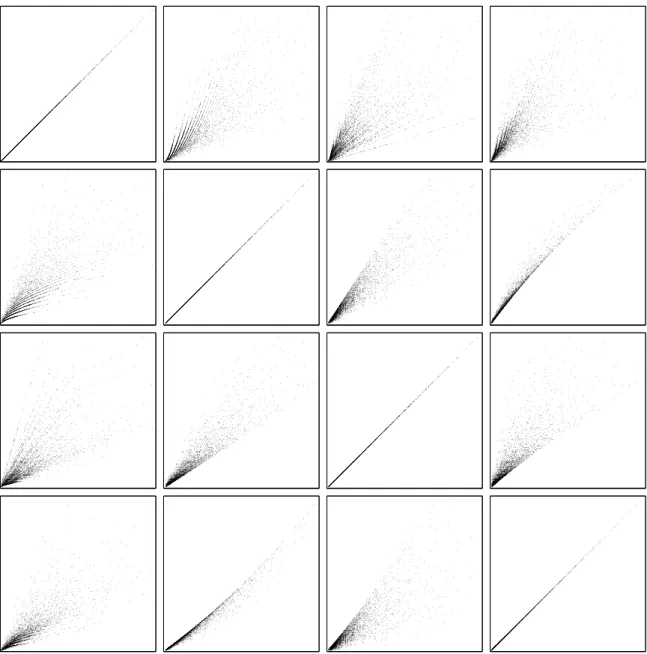
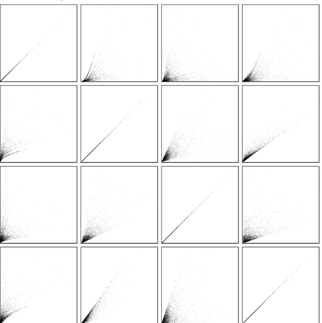
In order to examine how the association strength, the cosine, the inclusion index, and the Jaccard index are empirically related to each other, we analyzed each of the three data sets as follows. We first calculated for each combination of two objects the value of each of the four similarity measures. For each combination of two similarity measures, we then drew a scatter plot that shows how the values of the two measures are related to each other. The scatter plots obtained for the author data set and the term data set are shown in Figures 1 and 2, respectively. The scatter plots obtained for the journal data set look very similar to the ones obtained for the term data set and are therefore not shown. After drawing the scatter plots, we determined for each combination of two similarity measures how strongly the values of the measures are correlated with each other. We calculated both the Pearson correlation and the Spearman correlation. The Pearson correlation was used to measure the degree to which the values of two measures are linearly related, while the Spearman correlation was used to measure the degree to which the values of two measures are monotonically related. When calculating the Pearson and Spearman correlations between the values of two measures, we only took into
account values above zero.7 The correlations obtained for the three data sets are reported in
Tables 4, 5, and 6. In each table, the values in the upper right part are Pearson correlations while the values in the lower left part are Spearman correlations.
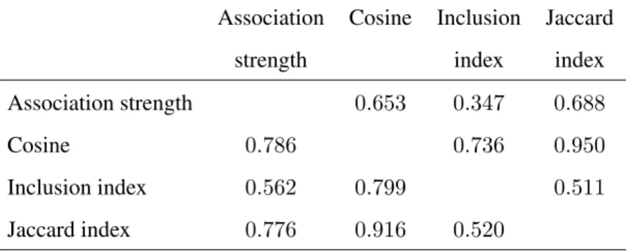
The scatter plots in Figures 1 and 2 clearly show that in practical applications there can be substantial differences between different direct similarity measures. This is confirmed by the correlations in Tables 4, 5, and 6. These results differ from the ones reported by Leydesdorff (2008), who finds no substantial differences between different direct similarity measures. The difference between our results and the results of Leydesdorff is probably due to the unusual nature of the data set studied in Leydesdorff, in particular the small number of objects in the data set (24 authors) and the division of the objects into two strongly separated groups (the information retrieval researchers and the scientometricians). When looking in more detail at the scatter plots in Figures 1 and 2, it can be seen that the similarity measures that are strongest related to each other are the cosine and the Jaccard index. The same observation can be made in Tables 4, 5, and 6. The relatively strong relation between the cosine and the Jaccard index has been observed before and is discussed by Egghe (2008), Hamers et al. (1989), and Leydesdorff (2008). Apart from the relation between the cosine and the Jaccard index, the relations between the different similarity measures are quite weak. This is especially the case for the relations between the association strength and the other three measures. Consider, for example, how the association strength and the inclusion index are related to each other in the term data set. As can be seen in Figure 2, a low value of the association strength sometimes corresponds with a high value of the inclusion index and, the other way around, a low value of the inclusion index sometimes corresponds with a high value of the association strength. This clearly indicates that the relation between the two measures is rather weak, which is confirmed by the correlations in Table 6. It is further interesting to compare our empirical results with the theoretical results presented by Egghe (2008). Egghe mathematically studies relations between various (weak and non-weak) set-theoretic similarity measures under the simplifying assumption that the ratio of
7If two objects have zero co-occurrences, all four similarity measures have a value of zero. Co-occurrence
matrices usually contain a large number of zeros (see Table 3). This leads to high correlations (close to one) between the values of the four similarity measures. We regard these high correlations as problematic because they do not properly reflect how the similarity measures are related to each other in the case of objects with a non-zero number of co-occurrences. To avoid the problem of the high correlations, we only took into account values above zero when calculating correlations between the values of the four similarity measures.
association strength
association strength
cosine inclusion index Jaccard index
cosine
inclusion index
Jaccard index
Figure 1: Scatter plots obtained for the author data set. In each plot, the lower left corner corresponds with the origin. The scales used for the different similarity measures are not the same.
association strength
association strength
cosine inclusion index Jaccard index
cosine
inclusion index
Jaccard index
Figure 2: Scatter plots obtained for the term data set. In each plot, the lower left corner corre-sponds with the origin. The scales used for the different similarity measures are not the same.
Table 4: Correlations obtained for the author data set.
Association Cosine Inclusion Jaccard
strength index index
Association strength 0.824 0.721 0.823
Cosine 0.913 0.929 0.987
Inclusion index 0.847 0.964 0.866
Jaccard index 0.920 0.994 0.931
Table 5: Correlations obtained for the journal data set.
Association Cosine Inclusion Jaccard
strength index index
Association strength 0.602 0.556 0.554
Cosine 0.892 0.800 0.971
Inclusion index 0.808 0.881 0.644
Jaccard index 0.832 0.952 0.708
Table 6: Correlations obtained for the term data set.
Association Cosine Inclusion Jaccard
strength index index
Association strength 0.653 0.347 0.688
Cosine 0.786 0.736 0.950
Inclusion index 0.562 0.799 0.511
the number of occurrences of two objects is fixed. He proves that, under this assumption, there exist simple monotonic (often linear) relations between many measures. However, especially for the inclusion index, the scatter plots in Figures 1 and 2 do not show such relations. Our empirical results therefore seem to indicate that the practical relevance of the theoretical results presented by Egghe might be somewhat limited.
The general conclusion that can be drawn from our empirical analysis is that there are quite significant differences between various direct similarity measures and, hence, that in practical applications it is important to use the measure that is most appropriate for ones purposes. In the next section, we discuss how an appropriate similarity measure can be chosen based on sound theoretical considerations. We focus in particular on the case in which a similarity measure is used for normalization purposes.
6 How to normalize co-occurrence data?
As we discussed in the previous sections, there are various ways in which similarities between objects can be determined based on co-occurrence data. The different types of similarity mea-sures that can be used are shown in Figure 3. The first decision that one has to make is whether to use a direct or an indirect similarity measure. If one decides to use a direct similarity measure, one then has to decide whether to use a probabilistic or a set-theoretic similarity measure.
We first briefly discuss the use of indirect similarity measures. As pointed out by Schneider and Borlund (2007a), from a statistical perspective the use of an indirect similarity measure is a quite unconventional approach.8 However, despite being unconventional, we do not believe that
the approach has any fundamental statistical problems. Appropriate indirect similarity mea-sures include the Bhattacharyya distance, the cosine,9and the Jensen-Shannon distance. These
measures are known to have good theoretical properties (Van Eck and Waltman, 2008). A very popular indirect similarity measure, especially for author co-citation analysis (e.g.,
Mc-8A similar approach is sometimes taken in psychological research (e.g., Rosenberg and Jones, 1972; Rosenberg,
Nelson, and Vivekananthan, 1968). In the psychological literature, there is some discussion about the advantages and disadvantages of this approach (Drasgow and Jones, 1979; Simmen, 1996; Van der Kloot and van Herk, 1991).
9There are two different similarity measures, a direct and an indirect one, that are both referred to as the cosine.
Here we mean the cosine as discussed by, for example, Ahlgren et al. (2003) and Van Eck and Waltman (2008). This is a different measure than the one defined in (6).
(Weak) set-theoretic similarity measures Similarity measures Direct similarity measures Indirect similarity measures association strength Bhattacharyya distance cosine Jensen-Shannon distance Probabilistic similarity measures cosine inclusion index Jaccard index generalized similarity index
Figure 3: Different types of similarity measures.
Cain, 1990; White and Griffith, 1981; White and McCain, 1998), is the Pearson correlation. However, this measure does not have good theoretical properties and should therefore not be used (Ahlgren et al., 2003; Van Eck and Waltman, 2008). The chi-squared distance, which is proposed as an indirect similarity measure by Ahlgren et al. (2003), also does not have all the theoretical properties that we believe an appropriate indirect similarity measure should have (Van Eck and Waltman, 2008). We note that theoretical studies of indirect similarity measures can also be found in the psychometric literature (e.g., Zegers and ten Berge, 1985). In this literature, the cosine is referred to as Tucker’s congruence coefficient.
In the rest of this section, we focus our attention on the use of direct similarity measures. Direct similarity measures determine the similarity between two objects by taking the number of co-occurrences of the objects and adjusting this number for the total number of occurrences of each of the objects. In scientometric research, when a direct similarity measure is applied to co-occurrence data, the aim usually is to normalize the data, that is, to correct the data for differences in the number of occurrences of objects. This brings us to the main question of this paper: How should co-occurrence data be normalized? Or, in other words, which direct similar-ity measures are appropriate for normalizing co-occurrence data and which are not? We argue that co-occurrence data should always be normalized using a probabilistic similarity measure. Other direct similarity measures are not appropriate for normalization purposes. In particular,
set-theoretic similarity measures should not be used to normalize co-occurrence data.
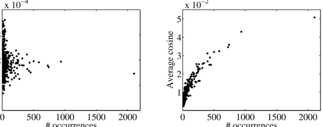
To see why probabilistic similarity measures have the right properties for normalizing co-occurrence data, recall from Section 4 that the number of co-co-occurrences of two objects can be seen as the result of two independent effects, the similarity effect and the size effect. As we discussed in Section 4, probabilistic similarity measures correct for the size effect. This follows from Property 4.2. Set-theoretic similarity measures do not have this property, and they therefore do not properly correct for the size effect. As a consequence, set-theoretic sim-ilarity measures have, on average, higher values for objects that occur more frequently (see also Luukkonen et al., 1993; Zitt et al., 2000). The values of probabilistic similarity measures, on the other hand, do not depend on how frequently objects occur. This difference between set-theoretic and probabilistic similarity measures can easily be demonstrated empirically. In Figure 4, this is done for the term data set discussed in the previous section. (The author data set and the journal data set yield similar results.) The figure shows the relation between on the one hand the number of occurrences of a term and on the other hand the average similarity of a term with other terms. In the left panel of the figure, similarities are determined using a probabilistic similarity measure, namely the association strength. In this panel, there is no substantial correlation between the number of occurrences of a term and the average similarity of a term (r =−0.069,ρ=−0.029). This is very different in the right panel, in which similar-ities are determined using a set-theoretic similarity measure, namely the cosine. (The inclusion index and the Jaccard index yield similar results.) In the right panel, there is a strong positive correlation between the number of occurrences of a term and the average similarity of a term (r = 0.839, ρ = 0.882). Results such as those shown in the right panel clearly indicate that set-theoretic similarity measures do not properly correct for the size effect and, consequently, do not properly normalize co-occurrence data. It follows from this observation that one should be very careful with the interpretation of similarities that have been derived from co-occurrence data using a set-theoretic similarity measure (see also Luukkonen et al., 1993; Zitt et al., 2000). Moreover, when such similarities are analyzed using multivariate analysis techniques such as multidimensional scaling or hierarchical clustering, one should pay special attention to possible artifacts in the results of the analysis. When using multidimensional scaling, for example, it is our experience that frequently occurring objects tend to cluster together in the center of a solution.
# occurrences
Average association strength
0 500 1000 1500 2000 1 2 3 x 10⁻⁴ # occurrences Average cosine 0 500 1000 1500 2000 1 2 3 4 5 x 10⁻²
Figure 4: Relation between on the one hand the number of occurrences of a term and on the other hand the average similarity of a term with other terms. In the left panel, similarities are determined using the association strength. In the right panel, similarities are determined using the cosine.
To provide some additional insight why probabilistic similarity measures are more appro-priate for normalization purposes than set-theoretic similarity measures, we now compare the main ideas underlying these two types of measures. Suppose that we are performing a co-word analysis and that we want to determine the similarity between two words, wordiand word j. We consider two hypothetical scenarios, to which we refer as scenario 1 and scenario 2. The scenarios are summarized in Table 7, and they are illustrated graphically in the left and right panels of Figure 5. In each panel of the figure, the light gray rectangle represents the set of all documents used in the co-word analysis, the dark gray circle represents the set of all documents in which wordioccurs, and the striped circle represents the set of all documents in which word
j occurs. The area of a rectangle or circle is proportional to the number of documents in the corresponding set.
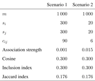
As can be seen in Table 7 and Figure 5, in scenario 1 words i andj both occur quite fre-quently, while in scenario 2 they both occur relatively infrequently. In both scenarios, however, the relative overlap of the set of documents in which word ioccurs and the set of documents in which word j occurs is the same. That is, in both scenarios word i occurs in 30% of the documents in which wordj occurs and, the other way around, wordjoccurs in30%of the doc-uments in which wordioccurs. Because the relative overlap is the same, set-theoretic similarity measures, such as the cosine, the inclusion index, and the Jaccard index, yield the same similar-ity between wordsiandjin both scenarios (see Table 7). This is a consequence of Property 3.2
Table 7: Summary of two hypothetical scenarios in a co-word analysis. Scenario 1 Scenario 2 m 1 000 1 000 si 300 20 sj 300 20 cij 90 6 Association strength 0.001 0.015 Cosine 0.300 0.300 Inclusion index 0.300 0.300 Jaccard index 0.176 0.176
Figure 5: Graphical illustration of two hypothetical scenarios in a co-word analysis. Scenario 1 is shown in the left panel. Scenario 2 is shown in the right panel.
discussed in Section 3. At first sight, it might seem a natural result to have the same similarity between wordsiandj in both scenarios. However, we argue that this result is far from natural, at least for normalization purposes.
We first consider scenario 1 in more detail. In this scenario, wordsiandjeach occur in30%
of all documents. If there is no special relation between wordsiandj and if, as a consequence, occurrences of the two words are statistically independent, one would expect the two words to co-occur in approximately 30% ×30% = 9% of all documents. As can be seen in Table 7, wordsiand j co-occur in exactly 9% of all documents. Hence, occurrences of wordsi andj
seem to be statistically independent, at least approximately, and there seems to be no strong relation between the two words.
We now consider scenario 2. In this scenario, words iand j each occur in2% of all doc-uments. If occurrences of words i and j are statistically independent, one would expect the two words to co-occur in approximately0.04%of all documents. However, words iandj co-occur in0.6%of all documents, that is, they co-occur 15times more frequently than would be expected under the assumption of statistical independence. Hence, there seems to be a quite strong relation between wordsiandj, definitely much stronger than in scenario 1.
It is clear that set-theoretic similarity measures yield results that do not properly reflect the difference between scenario 1 and scenario 2. This is because set-theoretic similarity measures are based on the idea of measuring the relative overlap of sets instead of the idea of measur-ing the deviation from statistical independence. Probabilistic similarity measures, such as the association strength, are based on the latter idea, and they therefore yield results that do prop-erly reflect the difference between scenario 1 and scenario 2. As can be seen in Table 7, the association strength indicates that in scenario 2 the similarity between wordsiandj is15times higher than in scenario 1. This reflects that in scenario 2 the co-occurrence frequency of words
iandj is15times higher than would be expected under the assumption of statistical indepen-dence while in scenario 1 the co-occurrence frequency of the two words equals the expected co-occurrence frequency under the independence assumption.