Understanding Community Structure for
Large Networks
by
Beate Franke
A dissertation submitted in partial fulfillment of the requirements for the degree of
Doctor of Philosophy
of
University College London.
Supervisor: Patrick J. Wolfe Department of Statistical Science
University College London September 30, 2016
I, Beate Franke, confirm that the work presented in this thesis is my own. Where information has been derived from other sources, I confirm that this has been indicated in the thesis.
September 30, 2016
Abstract
The general theme of this thesis is to improve our understanding of community structure for large networks. A scientific challenge across fields (e.g., neuroscience, genetics, and social science) is to understand what drives the interactions between nodes in a network. One of the fundamental concepts in this context is community structure: the tendency of nodes to connect based on similar characteristics.
Network models where a single parameter per node governs the propensity of connection are popular in practice. They frequently arise as null models that indicate a lack of commu-nity structure, since they cannot readily describe networks whose aggregate links behave in a block-like manner. We generalize such a model called the degree-based model to a flexible, nonparametric class of network models, covering weighted, multi-edge, and power-law net-works, and provide limit theorems that describe their asymptotic properties.
We establish a theoretical foundation for modularity: a well-known measure for the strength of community structure and derive its asymptotic properties under the assumption of a lack of community structure (formalized by the class of degree-based models described above). This enables us to assess how informative covariates are for the network interactions. Modular-ity is intuitive and practically effective but until now has lacked a sound theoretical basis. We derive modularity from first principles, and give it a formal statistical interpretation. Moreover, by acknowledging that different community assignments may explain different aspects of a net-work’s observed structure, we extend the applicability of modularity beyond its typical use to find a single “best” community assignment.
We develop from our theoretical results a methodology to quantify network community structure. After validating it using several benchmark examples, we investigate a multi-edge network of corporate email interactions. Here, we demonstrate that our method can identify those covariates that are informative and therefore improves our understanding of the network.
Acknowledgments
Four great years go to an end of intense discussions, hard work, sleepless nights and many incredibly rewarding moments when I finally truly understood.
I would first like to thank my supervisor Professor Patrick Wolfe for his support, guidance, and for hours of insightful discussions. Patrick’s passion for mathematics and rigor has often motivated me. I strongly appreciate the many doors Patrick has opened for me, and all the exceptional experiences that came with it. I am grateful to Patrick for teaching me to believe in myself, to live up to my potential and for encouraging me to reach even higher.
I would also like to thank the Stochastic Processes Group at UCL, for their curiosity and the great seminars with many enlightening questions. A special mention is needed for Professor Sofia Olhede, Dr Pierre-Andr´e Maugis, and Dr Simon Lunagomez. To Sofia for her great advice, creativity and energy. To Pierre-Andr´e and Simon for many inspiring discussions, for sharing their experience, and always readily lending an ear.
I am sincerely grateful to everyone at the UCL Department of Statistical Science for cre-ating an open, and stimulcre-ating environment, where you can always ask and where people are happy to help. I enjoyed our lunchtimes, chats over tea and Friday nights at ULU. I particularly would like to thank Dr Codina Cotar, Professor Tom Fearn, and Dr Ioanna Manolopoulou for career advice and general support; as well as Dr Ioannis Kosmidis, and Dr Yvo Pokern for in-spiring conversations. Special thanks go to Anne-Marie, Rodrigo, Anna, Katrin, Hannah and Verena for moral support; and to Bibi, Mike, Michael, James, Rui, Bryan, Francesco, and Sam for making sure I see more than my books during my time at UCL.
I also greatly acknowledge the funding of my PhD studentship by the UCL Department of Statistical Science. I thank Dr Leon Danon for sharing the data on jazz musicians from [59] and Mar´ıa Dolores Alfaro Cuevas for producing Figure 4.1.
I am thankful to Professor Nancy Reid for inviting me to participate for three months in the Fields program on big data. The people I met there and the talks and discussions I attended, widened my professional horizon. Special thanks go here to Dr Jean-Franc¸ois Plante and Dr Ribana Roscher. On a similar note, I wish to thank Dr Aaron Clauset, Professor Mason Porter
and Dr David Kempe for organizing the Mathematical Research Community on Networks; in particular Mason for career advice and general support. I thank Dr Bailey Fosdick and Professor Gesine Reinert for the interesting discussions.
I also wish to thank Professor Iris Pigeot, and Dr Ronja Foraita who guided me during the very early stages of my career. It is due to Professor Pigeot’s passion for statistics and the joint work with Ronja that I found my way to statistics.
I am very grateful to have met Tianmiao and Lisanne, who became very dear to me within the past four years. Thanks for sharing your thoughts and challenges, and making me take a break. A problem shared is a problem halved.
Thanks to my beloved friends Anki, Caro, Janne and Mary for sharing the good and the bad times with me, for always being understanding, and visiting me across the miles—with or without my consent. For our friendship, it seems that time and space do not matter.
I am eternally indebted to my family Marco, Na, Max Mustermann, Moni, Andi, Thore, Geli, Henna, Melanie, Guido, Marlene, Caspar, Marianne, Helmut and Ute for always support-ing me in whatever I want to do; for never misssupport-ing an opportunity to cheer me up and for always making me feel loved and welcome at home. Special thanks to Marlene, Caspar and Thore for reminding me that there are more important things in life.
Finally, I am deeply thankful to my partner Matthias for encouraging me to find my own way, and be myself. I am grateful for your confidence, peace of mind, and attitude that there is no mountain too high. Thanks for being there for me, for believing in me and for making me laugh, even in moments when it seems impossible. I love you.
Contents
1 Introduction 14
1.1 Motivation . . . 14
1.1.1 Networks and community structure . . . 14
1.1.2 Motivating examples of networks in science . . . 15
1.2 Preliminaries . . . 16 1.2.1 Definitions . . . 16 1.2.2 Concepts . . . 18 1.3 Properties of networks . . . 19 1.3.1 Local properties . . . 19 1.3.2 Global properties . . . 23 1.4 Modeling of networks . . . 25 1.4.1 Node dependence . . . 26 1.4.2 Edge dependence . . . 30
1.5 Contributions of the thesis and their context . . . 32
1.6 Outline . . . 34
2 Literature review of prominent challenges in network modeling 35 2.1 Network models with higher dimensionality . . . 35
2.1.1 Dynamic networks . . . 36
2.1.2 Multi-layer networks . . . 41
2.2 Quantifying goodness-of-fit of network models . . . 41
2.2.1 The parametric bootstrap . . . 41
2.2.2 AIC and BIC . . . 42
2.2.3 Bayes factor . . . 42
2.2.4 Likelihood approach . . . 43
2.3 Comparison between observed networks . . . 43
2.3.2 Test for an agreement in the generating model . . . 45
2.4 Clustering in networks . . . 45
2.4.1 Model-based community detection . . . 46
2.4.2 Heuristic community detection . . . 48
2.4.3 Identification of the number of communities . . . 50
2.5 Clustering in networks via modularity . . . 52
2.5.1 Introduction . . . 53
2.5.2 Properties . . . 54
2.5.3 Related work . . . 55
3 Nonparametric family of degree-based models 57 3.1 Definition of a nonparametric family of degree-based models . . . 58
3.2 Properties of the estimator of a node’s centrality . . . 58
3.2.1 A limit theorem for the estimator of a node’s centrality . . . 59
3.2.2 A confidence interval for the estimator of a node’s centrality . . . 62
3.2.3 Multivariate limit theorem . . . 64
3.3 Properties of the estimator of an edge expectation . . . 66
3.3.1 Weak consistency of the estimator of an edge expectation . . . 66
3.3.2 A limit theorem for the estimator of an edge expectation . . . 67
3.4 Illustrative simulations . . . 69
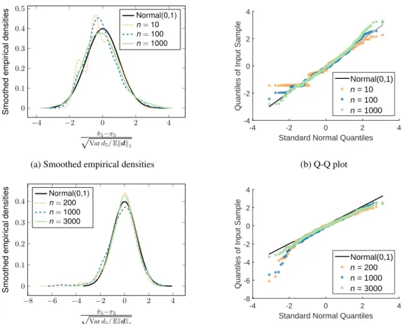
3.4.1 The limit theorem for the estimator of a node’s centrality . . . 70
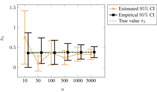
3.4.2 The confidence interval for the estimator of a node’s centrality . . . 72
3.5 Discussion . . . 73
4 Significance of a community structure under degree-based models 75 4.1 Modularity in the presence of observed community structure . . . 76
4.2 Properties of modularity . . . 78
4.2.1 Modularity reflects within- and between-group edges . . . 78
4.2.2 A limit theorem for modularity . . . 83
4.3 Illustrative simulations for the limit theorem for modularity . . . 86
4.3.1 Simple networks . . . 87
4.3.2 Multi-edge networks . . . 88
Contents 11
5 Data analysis 92
5.1 A methodology to quantify network structure . . . 92
5.2 Validating the methodology on benchmark examples . . . 93
5.2.1 Description of the data . . . 93
5.2.2 Elicitation of the model and deriving thep-values . . . 94
5.2.3 Results . . . 96
5.3 Evaluating communities in a multi-edge email network . . . 96
5.3.1 Description of the data . . . 97
5.3.2 Elicitation of the model and deriving thep-values . . . 99
5.3.3 Results . . . 100
5.4 Discussion . . . 101
6 Summary, discussion, and future work 103 6.1 Summary of our contributions . . . 103
6.2 Discussion and future work . . . 104
6.2.1 Community structure in networks . . . 104
6.2.2 Network models with higher dimensionality . . . 105
6.2.3 Quantifying goodness-of-fit of network models . . . 105
A Mathematical preliminaries 107 A.1 Probabilistic order notation . . . 107
A.2 Standard results on convergence of random variables . . . 108
B Supporting material for Chapter 3 111 B.1 Lemmas for proofs in Chapter 3 . . . 111
B.2 Simulations illustrating theorems in Chapter 3 . . . 121
C Supporting material for Chapter 4 127 C.1 Lemmas for the proofs in Chapter 4 . . . 127
C.2 Simulations illustrating theorems in Chapter 4 . . . 145
D Supporting material for Chapter 5 149 D.1 Likelihood functions for model comparison . . . 149
1.1 Toy example illustrating adjacency matrix, degree, and communities . . . 17 1.2 Simulations to illustrate the two types of variation in networks . . . 19 1.3 Visualization of the power law behavior of the degree sequences . . . 20 1.4 Toy example to illustrate the difference between four centrality measures . . . . 21 1.5 Toy example to illustrate network motifs . . . 22 1.6 Toy example to illustrate node-dependent and edge-dependent network models 25 1.7 A friendship network illustrated for four community assignments . . . 33 2.1 Toy example to illustrate dynamic networks . . . 36 3.1 Simulations of the estimator of the centrality of node5for a sparse network . . 71 3.2 A confidence interval for the estimator of a node’s centrality . . . 72 4.1 Decomposition of a network of books in within- and between-group edges . . . 78 4.2 The large-sample distribution of modularity for simple, sparse networks . . . . 87 4.3 The large-sample distribution of modularity for multi-edge, sparse networks . . 89 5.1 A multi-edge corporate email network illustrated for four covariates . . . 97 5.2 Model comparison for a multi-edge network for maximum-likelihood fits . . . 98 B.1 Simulations for the estimator of the centrality of node5for a dense network . . 122 B.2 Simulations of the estimator of the centrality of node17for a dense network . . 123 B.3 A confidence interval for the estimator of a node’s centrality for a dense network 124 B.4 Simulations of the estimator of the edge expectation for a sparse network . . . 125 B.5 Simulations of the estimator of the edge expectation for a dense network . . . . 126 C.1 The large-sample distribution of modularity for simple, dense networks . . . . 145 C.2 The large-sample distribution of modularity for simple, sparse networks . . . . 146 C.3 The large-sample distribution of modularity for Erd˝os-R´enyi networks . . . 147 C.4 The large-sample distribution of modularity for multi-edge, dense networks . . 148
List of Tables
5.1 Validation of the model assumptions for four benchmark networks . . . 95 5.2 Analysis of four benchmark networks with covariates . . . 95 5.3 Goodness-of-fit for a multi-edge email network for maximum-likelihood fit . . 98 5.4 Analysis of a multi-edge corporate email network for multiple covariates . . . . 101
Introduction
In Chapters 1 and 2, we first motivate the problem addressed in this thesis and then review the literature starting with an introduction of networks, their properties and models; and finishing with a detailed discussion of the prominent challenges in network modeling. Having estab-lished a framework and given the right context, we then in Chapters 3–6 turn to our original contributions.
1.1
Motivation
1.1.1 Networks and community structure
In many sciences there has been a conceptual shift away from the study of individual entities and towards the analysis of entire systems—not least because of the technological advances that enable us to collect the corresponding data [79]. In every system, these entities interact either directly or induced as a summary of their dependencies. Networks give us a means to describe and analyze these interactions between entities. In contrast to classical statistics, networks allow us to model complex dependencies while assuming very little structure. For instance, there is no natural ordering and thus no geometry inherited in a network as it is in time series or spatial statistics.
The structure of many networks is strongly influenced by a natural division into commu-nities: sets of nodes with a stronger tendency to connect with nodes of the same set than with nodes of other sets. These communities are often implied by shared characteristics; but may also result from a similar function within the network. Much work has focused on identifying the single “best” community structure. However, one knows that clustering algorithms always return clusters, even when the input is purely noise. Hence, these “optimal” community assign-ments lack interpretability and present a barrier to understanding.
1.1. Motivation 15
Understanding the community structure of large networks is crucial to enable statistical modeling and inference on networks that come with provable guarantees. Scientists inevitably observe not only the network nodes and their connections, but also additional information in the form of covariates. By acknowledging that each covariate may explain different aspects of a network’s structure, we extend the concept of communities beyond its typical use in the search for a single “best” community assignment. We use covariates to define community assignments, and then deliver a method to quantify how well these communities explain the network’s structure.
1.1.2 Motivating examples of networks in science
Because of the ubiquity of networks, a contribution to network analysis has the potential to influence a wide variety of sciences. We now illustrate the importance of networks and com-munity structure on examples in neuroscience, genetics and social sciences.
Inneuroscience, particularly functional magnetic resonance imaging (fMRI), a volume containing the subject’s brain is discretized into three-dimensional voxels whose intensities are measured across time as an index for neural activity. Using the activity to define a similarity measure between voxels, fMRI images of the human brain are often modeled as networks [18, 36, 93]. Because of the size of fMRI data, and since they are naturally affected by structured spatial correlations and high-frequency noise, it is a common approach to combine voxels into functionally distinct regions of interest. This clustering of the network allows us to marginalize the structured short-range dependencies and to reduce the dimensionality [36]. Building up on this, Martino et al. [95] analyze the voxel intensities for two of the communities in patients suffering from bipolar disorder and show in a case-control study with 100 patients that the ratio of intensities is a potential biomarker to distinguish between depressive and mania. Ramot et al. [121] and others [130, 132] go one step further by conducting an intervention study on 16 patients, demonstrating that we may train patients (with and without their awareness) to change the functionality of the communities in the cortical network of the human brain.
Ingenetics, we identify proteins that are strongly associated with a disease and then de-sign drugs such that they modulate these proteins to perturb a disease state. Recent advances indicate that many effective drugs modulate multiple targets instead of a single protein [70, 122]. In this context, modeling protein interactions as a network enables us to analyze the consequences of a drug on the entire system: on the targeted protein; on other proteins that might influence the same phenotype; as well as on off-target proteins that lead to side-effects.
As a consequence, Hopkins and others [70, 122, 155] identify understanding the underlying protein interaction network as one of the main challenges of drug discovery. Vinayagam et al. [141] cluster the proteins into “indispensable”, “neutral”, or “dispensable” based on their centrality in the network. Based on a study of 1,547 cancer patients, the authors show that disease-causing mutations and drugs target primarily the indispensable proteins and identify 56 genes to be associated with cancer, of which 46 have previously not been known. In contrast, Wu et al. [148] cluster genes into overlapping communities corresponding to regions involved in coherent developmental programs. The authors demonstrate on a study of 1,640 images of the gene expression data of Drosophila (fruit fly) embryos that the communities identified using their unsupervised learning algorithm agree with the well-studied gap gene network.
Social networksof people and their interactions have probably the highest public aware-ness, not least due to popular examples such as Facebook and LinkedIn. They also have one of the longest academic histories with scientific contributions dating back at least to the 1930’s [101]. Of particular importance in social networks is homophily: the tendency of nodes to connect in communities of similar nodes [98]. Kearns et al. [76] exploit homophily to address privacy issues in a clustering task in the context of counterterrorism. The authors cluster people in a social network into target and non-target communities based on their connections. While protecting the privacy rights of non-target individuals, the authors minimize the number of tests; e.g., surveillance, needed to clarify a node’s affiliation for certain. Paluck et al. [118] conduct an intervention study to promote anti-conflict behavior in a social network of 56 schools with 24,191 students. While randomization is crucial to the result, the authors first block for pre-defined community structures; e.g., gender and grade, before randomly selecting schools and students for the intervention. The authors thereby adjust for homophily. Comparing interven-tion schools against the controls, the disciplinary reports of student conflicts reduced by 30% over 1 year. Thus, the authors demonstrate that influencing a few individuals in a network may be sufficient to cause a behavioral change in the majority of the nodes, when adjusting for homophily.
1.2
Preliminaries
1.2.1 DefinitionsWe define agraph(i.e., network)G = (V, E)as a tuple of the set of nodesV and the set of edgesE ⊆V ×V. We call the number of nodesn=|V|thesizeof the graph and thedensity
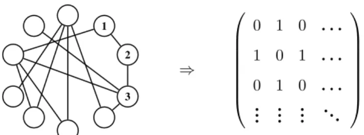
1.2. Preliminaries 17 1 2 3 ⇒ 0 1 0 . . . 1 0 1 . . . 0 1 0 . . . .. . ... ... . ..
(a) Each network may be represented by an adjacency matrix.
3
(b) The degree of a node is the sum of its connections(d3= 4).
(c) Community assignments are partitions of the nodes.
Figure 1.1: Toy example of a binary network with 10 nodes. denotes the proportion of observed edgesN over the number of possible edges:
den(G) =N. n(n−1)
2 .
The density of a network lies between0and1, with0being the empty network of no edges and
1if there is an edge between all pairs of nodes.
Representing by Aij ≥ 0 an edge between nodes i and j, we can describe the entire
network using its adjacency matrixA= (Aij)i,j=1,...,n. We call a graphbinaryif two nodesi
andjare either connected(Aij = 1), or not(Aij = 0). Figure 1.1a illustrates how to convert
a binary network into an adjacency matrix for a toy example. We will see in Chapters 3 and 4 that adjacency matrices make generalizations of graphs easy and are useful for the analyses of networks.
Each of the networks in the introduction can formally be described as a graph. We group these networks by the nature of their relationships. A prominent binary graph is a sim-ple network where we assume in addition to Aij ∈ {0,1}: the relationships are symmetric (Aij =Aji,∀i, j); and there are no self-loops, i.e., a node cannot connect to itself(Aii= 0,∀i).
Friendship networks for instance are often modeled as simple graphs. Networks where two nodes can have more than one edge are calledmulti-edgenetworks; e.g., an email interaction network. When the connections between nodesiand j are quantified with a weight we call the networkweighted; and networks where the relationships are not symmetric are called
di-rected networks. For the scope of this thesis, we concentrate on undirected networks without self-loops (i.e.,Ais symmetric andAii= 0,∀i), unless otherwise specified.
As illustrated in Figure 1.1b, thedegreedi =Pj6=iAij denotes the number of connections
of nodei. The degree plays a central role for this work as we will see in Chapter 3 about the degree-based model. In practice, scientists often analyze the degree sequence of an observed network, which is a vector of all degrees sorted in non-decreasing order. To discuss community structure, we partition nodes intogroups(i.e.,communities) as illustrated in Figure 1.1c. The functiongdenotes thecommunity assignmentof the network such thatg(i)denotes the group of nodei.
Awalkon a graph is a sequence of alternating nodes and edges(ν0, e1, ν1, e2, ν2, . . . , νl);
where the edge ei+1 between nodes νi andνi+1 needs to be present in the network for i = 0, . . . , l. Thelengthof this walk is said to bel. Acycleis a walk of length at least three that starts and ends at the same node but does not pass through any other node twice. A pathis a walk without repeated nodes and edges. The distancebetween two nodes is the length of the shortest path connecting them where for weighted networks we calculate the sum of the weights. Thediameterof a graph is the longest distance between any two nodes in the graph.
A graph is calledconnected if there exists a walk from every node to every other node. Acomponentis a maximally connected subgraph; i.e., adding any other node to this subgraph would break the connectedness. The component of a graph that includes the largest number of nodes is called thelargest component. A graph where there is an edge between every two nodes is calledcompleteand a complete subgraph is called aclique. Inregulargraphs, every node has the same degree.
1.2.2 Concepts
In this work, we discussrandom networkswhere the edgesAij are random variables and we
understand an observed network as a realization of a random network. In this context, there are two different types of variation: Firstly, within a single network the behavior of the nodes varies across index; e.g., Figure 1.2a displays the degrees of all nodes of the same network. Secondly, when we draw several independent and identically distributed (iid) replicates from the same network model, the behavior of a specific node varies across trials; e.g., Figure 1.2b displays the degree of the53rdnode across800replicates. Both types of variation will be addressed in this work.
1.3. Properties of networks 19 0 500 1000 0 100 200 300 Node index Degree value
Degrees of a single trial Expected degrees Theoretical 95% CI
(a) In a single network across nodes.
Trial index 0 200 400 600 800 Degree value 80 100 120 140 160 Degrees of 800 trials Expected degree
(b) For the single node53across trials.
Figure 1.2: Two types of variation in networks: the degrees in simulated networks with1,000
nodes from a power law model (pij = 0.81(ij)−0.2for alli < j).
change when the number of nodesn grows. Formally, we consider asequence of networks {Gn= (Vn, En)}n∈
Nwith|V
n|=nand analyze how the properties ofGnchange asn→ ∞.
For instance, let us consider a student friendship network. Would we expect students in larger schools to have more friends? If we keep increasing the size of the school, will the number of friends keep increasing? Researchers agree that there is an upper limit to the number of people we can have an active social relationship with, the Dunbar’s number [46, 146]. In network terms, Dunbar’s number is an upper bound of the degree of every node. Note that all network properties may depend onn, e.g. the degreedni of nodei, but for notational convenience we omit the superscriptn.
1.3
Properties of networks
To analyze networks, we first need to describe them. In this section, we introduce several network properties that have frequently been observed in practice. These properties either ad-dress the local structure where we focus on connections within relatively small neighborhoods across the network; or the global structure where we identify statements that hold for the entire network. We now discuss several local and global properties consecutively.
1.3.1 Local properties
In many networks, we observe degree heterogeneity: there is a large variability between the degrees of the nodes of the same network; with some nodes having in order of magnitude more connections than the average degree. This phenomenon is often coined the scale-free
Sorted Node index 0 50 100 150 Degree value 0 10 20 30
(a) Political books
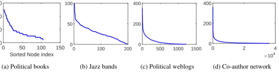
0 100 200 0 50 100 (b) Jazz bands 0 500 1000 1500 0 200 400 (c) Political weblogs #104 0 2 4 0 200 400 (d) Co-author network
Figure 1.3: Degree versus sorted node index: visualization of the power law behavior of the degree sequences of four binary networks.
behavior. In particular, in many networks the expected proportion of nodes withdi =kscales
approximately ask−β—thepower lawbehavior of the degree sequence [10]. Note that for many networks this holds only for the majority of the degrees, the exception being the degrees of lower value [32]. The power law behavior has been observed for instance for the internet, and social, and citation networks withβtypically varying between 2 and 3 [48, p. 11]. Figure 1.3 displays the sorted degrees of four networks: a network of books [108] where books are connected if they have frequently been purchased together; a network of jazz bands [59] where bands are connected if they have at least one band member in common; a network of political commentary websites (weblogs) [1] where weblogs are connected if they refer to each other; and a network of physicists [104] where physicists are connected if they have co-authored a manuscript. For more details on these datasets see Chapter 5.
Node centralityis a measure for the importance of a node in a network. In a social network, the most central person will be best to spread information or crucial to prevent a disease from spreading [28]. In economics, Diebold and Yilmaz use centrality (there called connectedness) to assess the risk attached to the default of economic institutions [42]. In a gene regulatory network, the centrality of a gene indicates how lethal its deletion would be [70]. There are many different centrality measures but they often build up on the following four: degree, closeness, betweenness, and eigenvector centrality; which we now introduce.
Thedegreecentrality of a node is measured by its degree
cD(i) =di,
and reflects the concept that the importance of a node is well described by the number of its di-rect connections. Since the degree is of importance to the work here, so is the degree centrality; as we will see in Chapter 3 about the degree-based model. Furthermore, Zerubavel et al. [152]
1.3. Properties of networks 21 3 4 5 6 1 2 7 8 9 10 11
Figure 1.4: Toy example to illustrate the difference between four centrality measures [79]. The coloring indicates the most central node according to the degree (red, node2), closeness (blue, node4), betweenness (green, node5), and eigenvector centrality (orange, node1).
identify brain regions that relate to affective valuation and social cognition in humans conduct-ing a fMRI study. The authors use the degree centrality as the base line measure for popularity of individuals. Paluck et al. [118] implement an intervention study in a social network in56
schools to test whether promoting positive behavior in a few nodes might be sufficient to change the behavior of the majority of the network (as mentioned above in Section 1.1). The authors report that the spread of community social norms is the most effective when the intervention is applied to the “social referents”—community members with high degree.
Theclosenesscentrality captures the notion that a node is central if it is closely connected to many other nodes; thereby taking into account more than the direct neighbors. The closeness centrality of nodeiis measured as the inverse of the distance (denoted by “dist”) of nodeito all other nodes [128]:
cCL(i) =
1 Pn
j=1dist(i, j) .
Mathematically, this distance is only defined in connected graphs. To circumvent this issue, we may report the closeness centrality conditioned on the largest component or for each component individually.
The betweennesscentrality measures how many paths go through a node. For instance if an edge represents a communication, the number of paths that go through a node counts how often a node can influence the information spreading through the network. Withs(j, l|i)
denoting the number of shortest paths between nodesj andlpassing throughi, Freeman [57] defines betweenness centrality of nodeias
cB(i) = X j6=l6=i s(j, l|i) Pn m=1s(j, l|m) .
If the shortest path is unique for all pairs of nodes,cB(i) counts the number of shortest paths
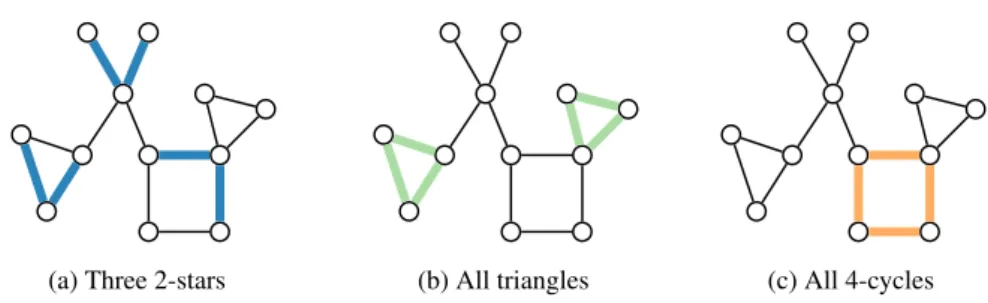
(a) Three 2-stars (b) All triangles (c) All 4-cycles
Figure 1.5: Toy example to illustrate network motifs. We display 2-stars: subgraphs with three nodes and two edges; triangles: complete subgraphs with three nodes; and 4-cycles: cycles of length four. Note, in Figure 1.5a we only highlight three out of many 2-stars for better visibility. Eigenvector centrality captures the notion of “prestige” where a node’s importance is judged by the importance of its neighbors. It is typically measured as a function of an eigen-vector of a linear system of equations related to the adjacency matrix. One of many examples of eigenvector centralities is defined by Bonacich [23] as
ceig(i) = 1 α X (i,j)∈E v(j),
whereαdenotes an eigenvalue of the adjacency matrixAandvthe corresponding eigenvector. Bonacich recommends to chooseαas the largest eigenvalue.
Figure 1.4 illustrates that although all four measures address centrality, they in fact mea-sure different quantities. These centrality meamea-sures may have different interpretations in prac-tice. For instance in protein interaction networks, pharmacologists are interested in identifying proteins that are correlated with gene expression dynamics, but that are not lethal; such that a medication can target these specific proteins. Both betweenness centrality and degree central-ity are associated with gene expression (betweenness centralcentral-ity stronger than degree centralcentral-ity) and lethality. However, nodes of medium to low degree centrality with a high betweenness centrality tend to be less likely to be lethal than the average protein [70].
In many networks, we observe that nodes tend to gather in “small neighborhoods”, such that they have more connections within their neighborhood than on average to all other nodes. One way to quantify this is theclustering coefficientof a graphGthat measures the proportion of 2-stars that close to form triangles. As illustrated in Figures 1.5a and 1.5b, 2-stars are sub-graphs with three nodes and two edges (∠); and triangles are complete subgraphs with three nodes (M). To be more precise, the clustering coefficientcl∈(0,1)is defined as
cl(G) = 1 |V0| X i∈V0 countM(i) count∠(i) ,
1.3. Properties of networks 23
wherecount(·)(i)denotes the count of occurrences of·centered at nodei; andV0denotes the set
of all nodes with at least two connections. In a network with a high clustering coefficient there is a strong tendency for 2-stars to form triangles. This phenomenon is also calledtransitivity. It is often observed in social sciences and commonly interpreted as “friends of friends tend to be friends” [112].
Comparing networks across sciences, we observe not only triangles but a variety of small subnetworks calledmotifs. The difference between two networks can be quantified by counting the occurrences of these motifs [100, 112]. For instance, for a subnetwork with three nodes there are two different motifs: 2-stars and triangles (see Figures 1.5a and 1.5b). While in social sciences we often observe transitivity, in gene regulatory networks and neuronal networks we observe in addition to transitivity an increased number of 4-cycles [100]. As illustrated in Figure 1.5c, 4-cycles are cycles of length four. We will return to the topic of motif counts in Section 2.3 in Chapter 2 on prominent challenges in network modeling.
1.3.2 Global properties
Stepping away from the node-centric view, we now discuss several network properties that are global. In many sciences, e.g. neuroscience, we observe functional units in networks that can be described as acommunity structureand may be used to reduce the dimensionality and noise of the data [36] (see Chapter 1.1). Formally, a community structure is a partition of the nodes into communities. Since we can partition the nodes arbitrarily, we denote a community structure as “informative” or “assortative” when there are more edges within communities than across communities. An informative community structure reflects a different aspect of the phe-nomenon described above that nodes tend to gather in small neighborhoods. In social sciences, this phenomenon is termed “homophily” and implies that connections between people of the same community occur at a higher rate than between communities because of the similarity of people of the same community [98].
The Harvard sociologist Stanley Milgram coined the termsmall-world propertyin 1967 when he conducted a study suggesting that every two people on this planet are only separated by at most six other people [99]. The fascination of this example results from the fact that this distance between two nodes is much smaller than we would expect at random (i.e., if all edges were placed uniformly at random). The small-world property was therefore formalized by Watts and Strogatz as a small average distance and a high clustering coefficient. While Milgram only studied social networks, Watts and Strogatz show that the small-world property in fact holds
for networks in many scientific fields; e.g., neural networks in neuroscience, power grids in electrical engineering, and collaboration networks in social sciences [145]. Formally, we talk about a small average distance when in a sequence of networks the expected average distance between two nodes scales asO(logn)[145]. The order notation is explained in Appendix A.1. In practice, scientists address this asymptotic property by computing the average distance of the largest component in the observed network (often a single snapshot) [79]. Watts and Strogatz introduce a generating model that leads to networks possessing the small-world property which we will discuss in more detail in Section 1.4.2.
Many properties of network models depend on thesparsity of the network: the relation between the number of edges and the number of nodes [20, 87]. For instance, let us assume a random network where an edge between every two nodes occurs equally likely with prob-abilityc/n(see Erd˝os-R´enyi graphs in Section 1.4.1). The constant cstrongly influences the number of edges in relation to the number of nodes and in other words, the sparsity of the net-work. At the same time, the value ofcdetermines whether the network is connected: Consider a sequence of networks where0 < c < 1. Then, the largest component includes with high probability at mostO(logn) nodes, leading to a network that is not connected. In contrast, if
1 < cthe largest component includes with high probability almost all nodes (Θ(n)). For an explanation of the notation see Appendix A.1. This phenomenon was first described by Erd˝os and R´enyi and is commonly referred to as the “emergence of the giant component”. For an overview about the work on the giant component see [20].
The definition of sparsity varies depending on the context. For this thesis, we use the definition by Bollob´as and Riordan [21, 22]. Recall thatndenotes the number of nodes andN
the number of edges. Then, a sequence of networks is dense:N = Θ n2,
sparse: N =o n2butN =ω(n),
extremely sparse:N = Θ(n).
For definitions ofΘ,o, andωsee Appendix A.1. In practice, we say a network is dense, sparse or extremely sparse if it seems reasonable to assume the observed network is a snapshot of such a sequence of networks. Bollob´as and Riordan call networks witho(n)edges (more sparse than extreme sparse networks) to be below the minimum sensible density since the average degree of a node would asymptotically go to 0. Most observed networks are sparse or extremely sparse [90].
1.4. Modeling of networks 25
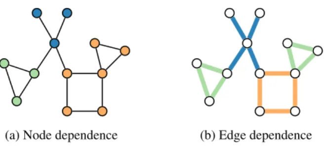
(a) Node dependence (b) Edge dependence
Figure 1.6: Toy example to illustrate the difference between node-dependent and edge-dependent network models. The coloring is defined by covariate in Figure 1.6a, and by motif in Figure1.6b. In both figures, things of the same color are modeled as stochastically equivalent.
1.4
Modeling of networks
So far, we have focused on the descriptive analysis of networks. To proceed to inference and prediction, we first need to introduce statistical models for networks. A statistical modelM for networks is a set of probability distributionsPrθ on the adjacency matrixA; i.e., withΨ
defining the set of all parametersθ, andΛthe set of all adjacency matrices, we obtain M={Prθ(A) :A∈Λ,θ∈Ψ}.
The nature of the relationships determines the set Λ. For instance, in a multi-edge net-work the entries of the adjacency matrix A are counts, so we obtain Λ = Nn≥×0n. In a
weighted network, in contrast, it follows that Λ = (0,1)n×n. We often have additional as-sumptions, e.g. in a simple network the edges are undirected and there are no self-loops:
Λ =
A∈ {0,1}n×n;AT =A, Aii= 0∀i .
As always, by modeling networks we encounter a trade-off between fit and complexity. If we model the network with as many parameters as there are possible edges(i.e.,n(n−1)/2), we achieve perfect fit but have not gained any insights (i.e., overfitting). Instead, we reduce the dimensionality where there are two fundamentally different approaches illustrated in Figure 1.6. First, one assumes node dependence: all edges are independent given the nodal attributes (see Figure 1.6a). For instance in email communications in companies, employees of the same department tend to communicate more with each other than with other departments (see data analysis in Section 5.3). Second, one assumes edge dependence: the probability distribution
Prθ only depends on the relation of the edges, independent of which nodes are involved (see
Figure 1.6b). For instance in social networks, we often observe an increased number of triangles since friends of friends tend to be friends (as mentioned in Section 1.3.1 on local properties).
We now discuss models of both approaches. 1.4.1 Node dependence
Since our work is focused on community structure, we categorize the models here into two types: those with a lack of community structure and those that support community structure.
Models with a lack of community structure
The Erd˝os-R´enyi graph G(n, p) is the simplest and probably most studied model for simple networks [49, 58]. It assigns an edge to each pair of distinct nodes independently with the same probabilityp ∈(0,1). It thereby models all nodes as stochastically equivalent; e.g., all nodes have the same expected degree. Thus across nodes, there is a lack of degree heterogeneity compared to what is frequently observed in practice (see Section 1.3).
To incorporates degree heterogeneity, thedegree-basedmodel allows for diverse propensi-ties to connect across nodes [31]. It assigns each node a single nonnegative weightwito model
the success probability of an edge between nodesiandjin a binary network as
pij = wiwj kwk1, withkwk1 = n X i=1 wi.
All edges are assumed to be conditionally independent given the parameters. To ensure that
0 ≤ pij ≤ 1, the weights are constrained tomaxlw2l < kwk1. If self-loops are allowed, the
expected degree of nodeiis equal to its weightwi and the model is therefore often referred to
as random graph with given (expected) degrees.
A special case of this model arepower law networks wherewi ∝ i−γ with γ ∈ (0,1),
introduced to match the power law behavior of degree sequences often observed in practice (see Section 1.3). Chung and Lu [31] compute the average distance and diameter of networks generated by the degree-based model, and show that for the special case of power law networks we obtain the small-world property. To be more precise, for a sequence of networks with
γ ∈ (0.5,1)—a range often observed in practice [10, 31, 32, 48]—the average distance is almost surelyO(log logn)[31].
To fit the degree-based model, Perry and Wolfe [119] estimate the edge probabilities as
ˆ pij =
didj
kdk1.
Recall that di denotes the degree of node i. The authors show that this estimator is a
1.4. Modeling of networks 27
explicit constants to check the sparsity assumption and give upper bounds for the relative error of the estimator in the least sparse case. The upper bound improves as the network becomes more sparse.
Olhede and Wolfe [116] analyze the degree distribution under the degree-based model; both for power law networks, and foriidrandom weights. The authors change the parameteri-zation such that the constraints may be specified for each node separately to
pij =πiπj withπi =wi/ q
kwk1 ∈(0,1);
and thus, the edge probabilities are decoupled. In particular, for the special case of power law networks, the authors derive a central limit theorem for the estimatorsπˆi =di/
p
kdk1. Theconfiguration model, discussed extensively in the physics and mathematics literature, is strongly related to the degree-based model: It fixes the actual degrees to then generate the network at random with respect to the given degrees [114]. In contrast, the degree-based model fixes the expected degrees instead.
Models supporting community structure
One of the simplest models for community structure is thestochastic blockmodel[68]: a gen-eralization of the Erd˝os-R´enyi graph. The nodes are partitioned intoKsubsets, called blocks, and the probability of an edge between nodesiandj only depends on the group membership g∈ {1, . . . , K}n(see Section 1.2.1):
pij =ωg(i),g(j).
It thereby models all nodes of the same community as stochastically equivalent. The authors assume the group membership to be known a priori and derive a straightforward maximum likelihood estimator for the edge probabilities as the sample proportion. In the remainder of the article the authors introduce a generalization of the stochastic blockmodel to directed net-works. Aicher et al., Airoldi et al., and Latouche et al. provide generalizations of the stochastic blockmodel to weighted networks and mixed and overlapping memberships, respectively [2, 3, 82]. We will come back to the stochastic blockmodel under the assumption of unknown (latent) communities in Section 2.4 on community detection.
As the Erd˝os-R´enyi graph, the stochastic blockmodel lacks heterogeneity of degrees. The degree-corrected stochastic blockmodel[75] marries the concepts of community structure and degree heterogeneity by combining the stochastic blockmodel and the degree-based model. The
authors assume a multi-edge network and model the expected edge countsEAij:
EAij =πiπjωg(i),g(j)
whereπ = (π1, . . . , πn)T are the node-specific parameters andωg(i),g(j) only depends on the
group membership g. In contrast, all models presented so far assume binary networks and thus model edge probabilitiespij instead. The authors suggest a two-step procedure for model
fitting: a profile likelihood estimation for the parametersπandωconditioned ong, and then a heuristic algorithm to identify the optimal group membershipg. The authors avoid maximizing the likelihood over all possible group memberships since that is aN P-hard problem [24].
The latent space models introduce a latent (unobserved) space where each individual node ihas an unobserved (“latent”) position zi ∈ Rd [67]. The model assumes that nodes
that are close in the latent space and have common covariates are more likely to connect. The latent space is commonly chosen to be of lower dimension; i.e., d < n; adding parsimony and interpretability. Additional benefits are that the latent space model incorporates both local and global structure, and transitivity, and that it outputs a meaningful visualization [131]. The authors model the edgesAij as conditionally independent given the latent positionsziand the
covariatesxij using a logistic regression model; i.e., withβdenoting all parameters logitpij =β0+βxij− |zi−zj|.
The latent positions zi are modeled using diffuse independent normal priors: zij iid
∼
Normal(0,100). The corresponding log-likelihood as a function of the latent positions is not concave; and much caution must be taken to differentiate local from global maxima. The authors suggest Markov chain Monte Carlo algorithms to infer the latent positions and de-rive confidence regions. The latent positions provide a soft clustering of the nodes into d
clusters while regressing on covariates. The latent space model was extended to include ran-dom node-specific effects [66] using a mixed effects model (a generalized linear model with structural error terms); and community structure [63] by modeling the latent positions as a mixture ofNormal random vectors (see Section 2.4 on clustering in networks). Krivitsky et al. [81] combine all four effects: homophily based on common covariates, transitivity, random node-specific effects, and community structure into a single model. To test for the dependence between latent structure and covariates, and to predict missing values, Fosdick and Hoff [53] model the covariates and latent structures as random simultaneously.
Closely related to the latent space model is therandom dot product graph[66, 151]. As for the latent space model, each node has a latent positionzi∈Rd, where allzij are modeled asiid
1.4. Modeling of networks 29
random variables. In contrast to the latent space model, it is assumed thatziTzj ∈(0,1)for all i, jand the probability for an edgeAij is modeled as the inner product of the latent positions:
pij =zTi zj.
The random dot product graph exhibits scale-free behavior of the degree sequence and the small-world property (small average distance almost surely and a high clustering coeffi-cient) [151]. Sussman et al. [138] introduce an estimator for the latent positions Zb = ( ˆz1, . . . ,zˆn)T ∈ Rn×d. Let U SUT be the eigen-decomposition of AAT1/2, and define
S[d]∈Rd×dthe diagonal matrix of thedlargest eigenvalues andU[d]∈Rn×dthe matrix of the
corresponding eigenvectors. Then, assuming we know the dimensiondof the latent space we may estimate the latent positions as
b
Z=U[d]S 1/2 [d] .
The authors show weak consistency of the estimators: kzˆi −zik22 = oP(1) for each iwith
k.k2 being the Euclidean norm. Furthermore, the scaled residuals between estimated and true
latent positions converge in distribution to a mixture of multivariate Normal distributed ran-dom vectors [9]. For more results on the eigen-decomposition of matrices related to A see Section 2.4.2.
Under the assumption that all parameters are random, all network models stated above can be joined to a single class of models [15]: Agraphondefines a limiting object for simple random networks when the number of nodes goes to infinity. Let us assume that all nodes are exchange-able: the edge probabilities are invariant to relabeling of the nodes. Since then the adjacency matrix (in the limit){Aij}∞i,j=1is an exchangeable infinite array of random variables, we know
that it admits a representation in functionsf(ξi, ξj, α)withξi, ξj, αiid∼ Uniform(0,1)
(Aldous-Hoover theorem [4, 69]) and that this representation is unique up to measure-preserving trans-formations [41]. To allow for sparse networks, it is common practice to multiply the graphon by a scaling factor ρn > 0 that depends on n. Thus, we obtain the following model for
ex-changeable simple random networks:
Aij|pij ∼Bernoulli(pij),
pij =ρnf(ξi, ξj, α), ξi, αiid∼ Uniform(0,1).
(1.1) Since EAij =
R R
pijdξidξj = ρn, the parameterρn reflects the overall sparsity of the
net-work. Each observed(n×n) network is then a sub-network of the infinite-dimensional net-work modeled in Eq. (1.1). This class of models is closely related to exchangeable random graph models [4, 69, 90] and inhomogeneous random graphs [20].
The function f does not uniquely determine the probability density function of the net-work [14]. However, it is common to interpret a graphon instead as an equivalence class that includesf and all its measure-preserving transformations. Olhede and Wolfe [117] present a method to fit a graphon: the network histogram approximates the potentially smooth graphon by a piecewise constant generating function, the stochastic blockmodel, in the same way as a histogram approximates a probability distribution function or the Riemann sum approximates the integral of a continuous function.
Li et al. [89] incorporate network structure intoclassic regressionby introducing a penalty to encourage network cohesion. Assume we are interested in the influence of p covariates x1, . . . ,xp ∈Rnon an outcomey ∈Rn, and we know the binary network connections of the
participants (i.e. the adjacency matrixA∈ {0,1}n×n). Denoteα∈Rna node-specific effect, an error term and letX = (x1, . . . ,xp)∈Rn×p. Then the authors suggest to modelyas
y=Xβ+α+.
To estimate the coefficientsβ ∈ Rp of the association of the covariates with the outcome, the
authors minimize a penalized residual sum of squares: withλdenoting a tuning parameter,
L(α, β) =ky−Xβ−αk22+λ X
∀i,j:Aij=1
(αi−αj)2.
Under some regularity conditions, the authors provide upper bounds for the mean squared errors for both corresponding estimatorsαˆ andβ; and show thatˆ βˆis consistent.
1.4.2 Edge dependence
We here provide two examples of models that exploit edge dependencies; one with a lack of community structure and one that supports community structure. The aim is to give a brief introduction to an alternative modeling approach; different from all models used in this work.
A model with a lack of community structure
TheWatts-Strogatzmodel [145] is designed to possess the small-world property: a small aver-age distance and a high clustering coefficient. Watts and Strogatz begin with a network where each node is connected to itsrnearest neighbors (i.e., ar-regular graph); a network that tends to have very high transitivity. They then randomly reconnect each edge with probabilityp(while avoiding self-loops and multi-edges); introducing “short-cuts” that reduce the average distance in the graph. As a consequence, the model is a hybrid between a regular and an Erd˝os-R´enyi
1.4. Modeling of networks 31
graph, for which even for smallp we observe the small-world property. The Watts-Strogatz model is of particular importance to the analysis of information propagation and epidemic spread, since it allows for information to be transmitted quickly through the entire network only based on neighbor-to-neighbor communications. A discussion about epidemic spread and related work is beyond the scope of this thesis. In contrast to our work, these approaches assume the network to be non-random and analyze a random process on the network.
A model supporting community structure
Theexponential random graphmodel (ERGM) [54, 144] builds up on the concept of exponen-tial families and thereby naturally extends statistical regression to random networks. It models a simple networkG= (V, E)in terms of a setHof motifs:
f(A|θ) = 1 κexp X H∈H θHcH ! , (1.2)
withcH being a count of how often the motif H occurs in the networkA; and the
standard-ization constantκ = P
A∈Λexp( P
HθHcH). Originally, ERGMs included star and triangle
counts (see Figure 1.5). The formula in Eq. (1.2) implies that the density factorizes over the sub-graphsH ∈ H. For instance ifHincludes only the edge subgraph, we assume all edges to be iid. For more details on the independence assumptions onfimplied byHsee the Hammersley-Clifford theorem [12].
The main advantage of the ERGM is that it can represent a variety of structural tendencies, such as transitivity, and that its parameters are easy to interpret. However, fitting the model has proved to be challenging because of three main reasons. First, computing the standardization constantκis computationally infeasible for medium to large networks (n >30) [62] sinceκis a sum over the entire sample spaceΛ. Second, very different values ofθcan lead to essentially the same distributionf [27]. Third, ERGM models are degenerate: they put the majority of mass on the empty graph, the complete graph or a mixture of the two [62]. To overcome the degeneracy, Handcock [62], Hunter and Handcock [72], and Snijders et al. [136] introduce priors that restrict the parameter space to graphs that are neither empty nor complete. Chatterjee and Diaconis [27] deliver limiting results that identify when degeneracy occurs; and show that those graphs that are not degenerate often are indistinguishable from an Erd˝os-R´enyi graph in the limit (i.e. f(A|θ) →P f(G(n, p))asn→ ∞). Since computingκis time consuming even for moderately small networks, Chatterjee and Diaconis [27] provide analytical formulas forκ
these limitations, many researchers question the suitability of ERGMs for statistical inference on networks [27].
1.5
Contributions of the thesis and their context
After establishing a framework in the previous sections, we now can explain the original con-tributions of the thesis, and embed them in the wider context of networks. We establish a methodology to identify the key characteristics that determine a network’s structure. To do so, we firstly characterize a family of flexible, nonparametric models that naturally generalize the degree-based model mentioned in Section 1.4.1. Under such models, we secondly derive the theoretical foundation for modularity: an intuitive and practically effective measure of the strength of community structure; enabling us to decide which of the characteristics reflect the structure of the interactions in a network.
First, we generalize the degree-based model to a broad class of models including weighted, multi-edge, and power law networks. We fit such a model using the canonical estimatorEdAij =
didj/kdk1 for which Perry and Wolfe [119] show that it is close to the maximum likelihood
estimator for the special case of simple networks. We show thatEdAij is weakly consistent
forEAij and derive its asymptotic distribution under this broad class of network models. Our
results generalize work by Olhede and Wolfe [116] who show the asymptotic distribution for the special case of power law networks. All approaches and results presented above assume the edges to be either Bernoulli or Poisson distributed. In contrast, we take a nonparametric approach: using a single parameter per node, we model only the expectation of each edge. This allows for individual node-specific differences but avoids specific distributional assumptions on the edges. Our results therefore apply to a broader class of network models, allowing us to treat (among others) power-law networks, weighted networks, and those with multiple edges.
Second, we extend the concept of community structure to reflect the complexity of ob-served networks. Scientists inevitably observe not only network nodes and their connections, but also additional information in the form of covariates. Many analysis approaches fail to ex-ploit this information when attempting to explain network structure, and instead solely focus on identifying a single “best” community structure (e.g. latent space models [67, 53], stochas-tic block models [68] and degree-corrected stochasstochas-tic block models [75]; see Section 1.4.1). In recent works, researchers have started to use covariates to improve community detection (degree-corrected stochastic blockmodels [110], latent space models [67], modularity [153],
1.5. Contributions of the thesis and their context 33
(a) Race (b) Year in school
(c) Gender (d) Randomized
Figure 1.7: A student friendship network illustrated for four different community assignments, each defined by a covariate [53, 110, 124]; implemented using igraph [38].
ERGMs [50], see Section 2.4.1). However, the concept of a single best community assignment leads to a loss of interpretability and presents a barrier to understanding. We solve this problem, by acknowledging that each of several community assignments may describe different aspects of a network’s structure. To add interpretability, we define these community assignments based on covariates, and show how to decide which of these covariate-based community assignments leads to a valid summary of the network structure. In the student friendship network shown in Figure 1.7, for example, this means we can evaluate whether communities based on common gender, race, or year in school can explain the observed structure of the friendships.
Technically, we derive modularity from first principles, and give it a formal statistical interpretation. Effectively, modularity summarizes the difference between observed and ex-pected within-community edges under a model for no community structure. We derive the large-sample distribution of modularity under the nonparametric class of degree-based models, enabling us to compute ap-value for the significance of a covariate-based community structure. This provides for the first time an objective measure of whether or not a particular value of modularity is meaningful. As a result, we deliver a flexible, nonparametric approach to identify those covariates that reflect a network’s structure.
Papers and preprints
[56] Franke B, Wolfe PJ (2016) Network modularity in the presence of covariates.
arXiv:1603.01214.
1.6
Outline
The remaining thesis is organized as follows. We first review the literature about prominent challenges in network modeling, including community detection using modularity (Chapter 2). We then present our original contributions. We extend the degree-based model to a nonparamet-ric family and derive its asymptotic properties (Chapter 3). We establish a theoretical framework based on modularity to assess whether a covariate-based community assignment is informative for the intersections in a network (Chapter 4). Here, we show that the model underlying mod-ularity is a degree-based model and derive a bias-variance decomposition for modmod-ularity. This enables us to establish the asymptotic distribution of modularity and to deliver a p-value re-flecting the explanatory power of covariates on network connections. In Chapter 5, we turn the theory into a methodology to identify covariates that are informative for the connections in a network. After validating our method on four benchmark examples, we analyze email in-teractions in a multi-edge corporate email network identifying those covariates that reflect the network’s structure. We conclude this thesis with a discussion of the prominent challenges; and point out possible directions of follow-up research (Chapter 6).
Chapter 2
Literature review of prominent challenges in
network modeling
In this chapter, we present a literature review about the current challenges in network modeling. In Chapter 1, we have seen how to describe networks and how networks are modeled so far. Due to technological advances, the amount of data that we can store and process increases on a daily basis; allowing us to collect data that better reflect the complexity of nature. However, to actually gain insights from the data our network models must catch up to reflect the high dimensionality of the data (see Section 2.1). All network models enable us to draw inference from data, but for the results to be defensible we must be able to quantify the goodness-of-fit of network models (see Section 2.2). In science, it is common to collect more than one dataset and by understanding the agreements and differences, we gain insights on what are the driving forces. In Section 2.3, we describe the current state-of-the-art for networks in this regard. Having mentioned the complexity of the data above, clustering gives us a means to extract information from networks: identifying groups of nodes that have a stronger tendency to connect to each other than to other nodes. In Sections 2.4 and 2.5, we discuss different approaches for clustering in networks with a special emphasis on modularity because of its popularity and its importance for the thesis. Our review of the current challenges in network modeling is not exhaustive but we rather focus our discussion on the four topics motivated above that we find the most prominent.
2.1
Network models with higher dimensionality
We now review models that have an increased dimensionality compared to the more traditional models in Section 1.4. Modern technology enables us to collect data that are increasingly large
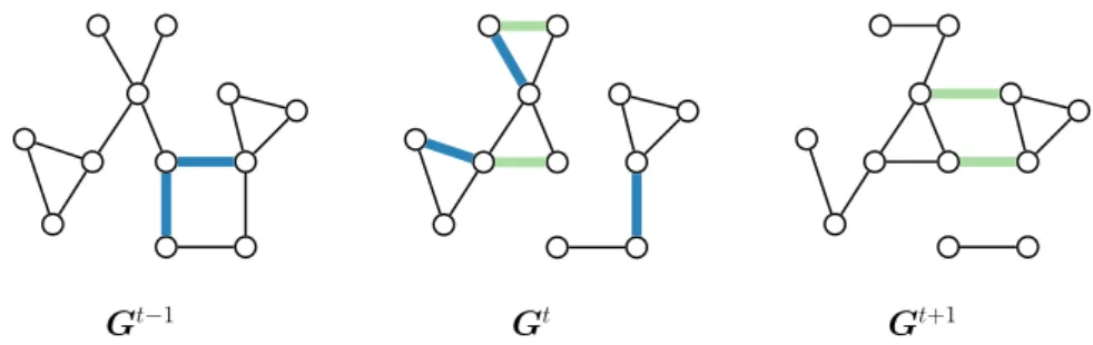
Gt−1 Gt Gt+1
Figure 2.1: Toy example to illustrate dynamic networks. Green and blue mark edges that appear in this time step or will disappear in the next time step, respectively. The node set is fixed. and diverse in structure—already in 2012 it was estimated that data collection was growing at 50% per year [55, 91]. Increasing the dimensionality of our models enables us to incorporate more of the complexity of the network data. The two leading approaches combine several networks into a single model. One assumes there to be a temporal dependence between the networks and the other allows for an arbitrary dependence in the spirit of a network of networks. We now discuss both approaches.
2.1.1 Dynamic networks
As illustrated in Figure 2.1, dynamic network modelsare a natural extension of the models described in Chapter 1.4 where networks are altered over time. For example, in social networks, friendships are made and lost over time, and in biological neural networks the activation of neurons is time-correlated; just to name a few. Formally, we assume a time series of networks
Gt:t= 1, . . . , T with Gt= V, Et
, and
At:t= 1, . . . , T
being the series of adjacency matrices. All approaches mentioned below assume the node setV
to be fixed over time; with the exception of the preferential attachment model.
One of the first statistical models for dynamic networks was introduced by Snijders in 1996 [134]. The authors model the adjacency matrixAtand the attributesCtof the nodes as Markov processes in continuous timet ∈ [0,∞). Denotet0 the present and t∗ ∈ [0, t0) all
previous time points. Then, the authors define
Pr At,Ct:t > t0 |t∗∈[0, t0)
= Pr At,Ct:t > t0 |t0
.
The authors assume that a change inAti orCitof connections and attributes of nodeioccurs at a rateλi(At,Ct)and model the waiting time until the next change by nodeias a negative
2.1. Network models with higher dimensionality 37
node has an incentive to optimize its attributes and connections to its own benefit. They model the decision making of nodeiusing a tension functionpi(At,Ct) that includes both a
deter-ministic and random component. The authors infer the parameters of the tension function and the rate of change using a method of moments based on parametric bootstrap and approximate the covariance matrix of the vector of estimators using the delta method. The authors point out that the approach is computationally expensive, lacks in statistical efficiency and caution the reader that the variance estimators might be instable.
Thepreferential attachment model describes a process of adding nodes, and connecting these to nodes with a probability proportional to their degree; leading to a “richer getting richer” phenomena and a power law degree sequence [10]. Although the preferential attachment model is understood as a single snapshot of a network, in contrast to multiple snapshots over time, it does describe a dynamic process of generating a network. In a similar way, we can describe the Watts-Strogatz model as a dynamic model (see Section 1.4.2). In contrast to the other models in this section, the preferential attachment model and the Watts-Strogatz model incorporate a change in the set of nodes but are not intended for statistical model fitting.
A generalization of therandom dot product graph for dynamic networksis provided by Lee and Priebe [84] where the authors aim to detect change points in the behavior of weighted net-works. The authors model a time series of networks with categorical edge weights in discrete-timet∈Nas a series of random dot product graphs derived from a finite-state Markov process in continuous-timeu:W ={w(u)∈ {1, . . . , d+ 1}n:u∈[0,∞)}. To be more precise, for nodesi, jand edge weightslit holds for the latent positionsZt = (z1, . . . ,zn)T ∈Rn×dthat
ztila.s.= Z t t−1 δwi(u)=ldu, forl= 1, . . . , d, Pr Atij =l|zt i,zjt = ziltztjl, forl6= 0; 1−Pd l=1ziltztjl, forl= 0;
independent for alli < j
Pr At=a|w(u), u≤t
= Pr At=a|Zt
.
The authors assume that the probabilities of the stochastic process W to take values in {1, . . . , d+ 1}change for a small community of nodes and they aim to detect the correspond-ing time point. The authors introduce two approximations to make the problem analytically tractable and show that their total variation distance under a dynamic random dot product graph is asymptotically small. Durante and Dunson [47] work on a strongly related model of a dynamic random dot product graph, where the latent positions evolve in a continuous
Markov process. Due to using a logistic link between the probability of an edge and the latent positions—the main difference—the authors obtain a computationally tractable formulation. They introduce an algorithm to both infer the posterior distribution and estimate the dimension of the latent space simultaneously.
In [131], Sewell and Chen generalize the latent space model for time-varying, sim-ple networks and thus, this work is strongly related to the dynamic random dot product graph by Lee and Priebe [84]. To be more precise, the authors model the latent positions Zt = zt
1, . . . ,ztn T
∈ Rn×d as a Markov process in discrete time t ∈ N. Denote Id the (d×d)-identity matrix, andθall parameters. Then, the authors define the initial distribution of the latent positions at timet= 1as
π Z1|θ = n Y i=1 Normal 0, τ2Id .
The transition probability is defined as
Pr Zt|Zt−1,θ= n Y i=1 Normal zit−1, σ2Id .
Networks at different time points are conditionally independent given the latent positions. At each time point, the edges are modeled using a latent space model: a logistic regression model with the distance in latent space being an explanatory variable and where we assume condi-tional independence of the edges given the latent positions and the parametersθ([67], see Sec-tion 1.4.1). The authors estimate the model parameters and the latent posiSec-tions using Markov chain Monte Carlo methods; where they provide approximations to speed up the algorithm. As an output, the authors deliver a temporal trajectory of each node in the latent space. Further-more, the authors address the problem of missing data, and prediction; and demonstrate their method on simulated and observed data.
Westveld and Hoff introduce a dynamic network regressionframework where the edges are modeled as conditionally independent using a generalized linear model with mixed ef-fects [147]. Denote st
i, rit the node-specific effects of node i as a sender and receiver,
re-spectively, andetij the residual error terms. The random effectssti, rti,etij are modeled using discrete-time Markov processes. Furthermore, denotext
ij the fixed effects, e.g., covariates, and hthe link function. The authors then model the adjacency matrix at timetas
E Atij|θijt
=h(θtij),
2.1. Network models with higher dimensionality 39
The authors provide Markov chain Monte Carlo algorithms for parameter estimation for Gaus-sian and binary networks and apply the method to data on international trade and militarized interstate disputes. This model partly builds up on the static, latent space model by Hoff [66], but it exchanges the latent positions against generic residual error terms.
To incorporate community structure into dynamic networks, Xing et al. [149] introduce a dynamic mixed membership stochastic blockmodel that generalizes the mixed membership stochastic blockmodel [2]. In the mixed membership stochastic blockmodel, a node may belong to multiple communities, each with a fractional membership; thereby combining the concepts of the stochastic blockmodel and the latent space model. DenoteBt = βklt k,l=1,...,K the probabilities to interact between nodes of communities k and l at time t. For the dynamic mixed membership stochastic blockmodel, the authors model for each node i the fractional membershipπt i = πti1, . . . , πtiK at timet: πti iid∼Logistic-Normal µt,Σt .
Thus,Σt determines the correlations of the memberships between nodes. For each edgeAij,
nodesiandjget assigned to a single community with a probability according to their fractional membershipsπitandπjt:
zlt∼Multinomial πtl,1
, forl=i, jindependent.
An edge between nodesiandjis then modeled:
Atij iid∼Bernoulli βlkt , ifzilt = 1, ztjk = 1.
Furthermore, the expected value ofπti is modeled as dynamic with transition matrixM: µ1∼Normal(ν,Ψ), µt∼Normal M µt−1,Ψ.
Here,Ψdetermines the correlation between the expected fractional memberships across time. In addition,Btis assumed to be time dependent. WithΦdenoting the variance of the probabil-ities to interact between communprobabil-ities, andba tuning parameter, we obtain
βlk1 ∼Logistic-Normal(ι,Φ), βlkt ∼Logistic-Normal bβlkt−1,Φ
.
The authors aim to infer the dynamics of the fractional membershipsπit, for all i, t; as well as the dynamical community relationsBt. Fitting the dynamic mixed membership stochastic
![Figure 1.4: Toy example to illustrate the difference between four centrality measures [79]](https://thumb-us.123doks.com/thumbv2/123dok_us/1985823.2794922/21.892.315.635.103.226/figure-toy-example-illustrate-difference-centrality-measures.webp)
![Figure 1.7: A student friendship network illustrated for four different community assignments, each defined by a covariate [53, 110, 124]; implemented using igraph [38].](https://thumb-us.123doks.com/thumbv2/123dok_us/1985823.2794922/33.892.284.656.115.551/figure-friendship-illustrated-different-community-assignments-covariate-implemented.webp)
![Figure 4.1: Decomposition of a network in within- and between-group edges: political books connected when frequently purchased together, where groups are defined by political align-ment [108]](https://thumb-us.123doks.com/thumbv2/123dok_us/1985823.2794922/78.892.278.565.111.395/figure-decomposition-network-political-connected-frequently-purchased-political.webp)