UCC Library and UCC researchers have made this item openly available. Please let us know how this has helped you. Thanks!
Title Simulated wave hydrodynamics and loading on an offshore monopile
Author(s) Edesess, Ariel J.
Publication date 2018
Original citation Edesess, A. J. 2018. Simulated wave hydrodynamics and loading on an offshore monopile. PhD Thesis, University College Cork.
Type of publication Doctoral thesis
Rights © 2018, Ariel J. Edesess.
http://creativecommons.org/licenses/by-nc-nd/3.0/
Embargo information Not applicable
Item downloaded
from http://hdl.handle.net/10468/7002
Simulated Wave Hydrodynamics
and Loading on an Offshore
Monopile
A Dissertation Presented by
Ariel J. Edesess
for the degree of
Doctor of Philosophy
in
Civil and Environmental Engineering
University College, Cork
Head of School: Prof. Liam Marnane Supervisors:
Dr. Denis Kelliher, Prof. Alistair G. L. Borthwick, Dr. Gareth P. Thomas
Thesis Declaration
This is to certify that the work I am submitting is my own and has not been submitted for another degree, either at University College Cork or elsewhere. All external references and sources are clearly acknowledged
and identified within the contents. I have read and understood the regulations of University College Cork concerning plagiarism.
Signed:
Date:
Acknowledgements
I am extremely grateful to my supervisors Dr. Denis Kelliher, Dr. Gareth Thomas and Prof. Alistair Borthwick. Your patience and encouragement kept me motivated, even when the path was the most uncertain. Thank you for the discussions and for helping me become a better researcher and thinker. I look forward to taking the skills I learned into the rest of my life. This research would not have been possible without financial and intellectual support from Alexis Billet, who got this project moving, EDF Energy, Marine and Renewable Energy Ireland (MaREI), Science Foundation Ireland (SFI) and UCC. Thank you to Dr. Tariq Dawood and Jack Egerton at EDF Energy for the opportunity to collaborate and for providing the data for this research. I am also grateful to Irish Centre for High-End Computing (ICHEC) for their support and use of FIONN, and to the OpenFOAM user community, especially Dr. Adam Johns, Dr. Rudolf Hellmuth, Dr. Lifen Chen and Matt Shepit. I also thank Prof. Vengatesan Venugopal and Dr. Ignazio Viola at The University of Edinburgh for the guidance and to Prof. Mike Hartnett at NUI Galway for providing me with a space to think. Thank you to my parents, Michael and Dyana, and my sister Hilary for the endless support, patience and the encouragement to keep asking questions, and finally, most of all to
´
If people do not believe that mathematics is simple, it is only because they do not realize how complicated life is.
Dissemination of Research
Published
• A. J. Edesess, D. Kelliher, A. G. L. Borthwick and G. P. Thomas. Improving global accessibility to offshore wind power through de-creased operations and maintenance costs: a hydrodynamic analy-sis. Energy Procedia: 2017 International Conference on Alternative Energy in Developing Countries (AEDCEE) 138: 1055–1060, Oc-tober 2017. doi: doi/10.1016/j.egypro.2017.10.107
• A. J. Edesess, D. Kelliher, A. G. L. Borthwick, G. P. Thomas. Off-shore monopile in the southern North Sea: Part 1, calibrated input sea state. Proceedings of the Institution of Civil Engineers -
Mar-itime Engineering, 170(3+4):122–132, 2017. doi: doi/10.1680/jmaen.2017.14
Accepted for Publication
• A. J. Edesess, D. Kelliher, A. G. L. Borthwick, G. P. Thomas. Offshore monopile in the southern North Sea: Part 2, simulated hydrodynamics and loading. Proceedings of the Institution of Civil Engineers - Maritime Engineering. 2018.
Selection of Oral Presentations
• “Improving Global Accessibility to Offshore Wind Power through Decreased Operations & Maintenance Costs: A hydrodynamic anal-ysis”. Presented at the 17th International Conference on
Alter-native Energy in Developing Countries and Emerging Economies (AEDCEE), Bangkok, Thailand. 25-26 May 2017
• “OpenFOAM simulations of irregular waves and free surface effects around a monopile offshore wind turbine”. Presented at the UK-Ireland OpenFOAM User Meeting. Dublin, UK-Ireland, 16-17 January 2017
• “Offshore wind farm maintenance operations: Analysis of free sur-face flow around a sursur-face-piercing monopile”. Presented at MaREI Symposium, Galway, Ireland. 1 November 2016.
• “Maintenance of Offshore Wind Farms: Crew Transfer Vessel Mo-tion Analysis”. Presented at EDF Renewables R&D Offshore Wind; London, United Kingdom. 5 August 2016.
• “Maintenance of Offshore Wind Farms: Crew Transfer Vessel Mo-tion Analysis”; presented at the NaMo-tional Wind Technology Cen-tre, National Renewable Energy Laboratory; Louisville, Colorado, USA. 27 July 2016.
• “Maintenance of Offshore Wind Farms: Crew Transfer Vessel Mo-tion Analysis”; presented at the 11th OpenFOAM Workshop; Guimar˜aes, Portugal. 26-30 June 2016.
• “Crew Transfer Vessel Motion Analysis: Maintenance of offshore wind farms”. Presented at the VI International Conference on Computational Methods in Marine Engineering - Marine 2015; Rome, Italy. 15-17 June 2015.
Abstract
Maintenance costs of offshore wind power, where fixed monopile sup-port columns make up the majority of wind turbine types, are up to three times higher than those associated with onshore wind power. High costs are exacerbated by difficulties accessing the turbines in their ma-rine environment. Safe transfer by crew transfer vessel (CTV) requires prediction of vessel motion whilst in contact with the turbine monopile. Future vessel motion prediction first requires analysis through analytical and numerical methods of the local hydrodynamic wave field and wave loading on the monpile turbine in ocean waves.
A location-dependent unidirectional sea state is represented by super-position of periodic waves with amplitude componentsan, obtained from
the spectral distribution of free surface displacement data from a single wave buoy located at the Teesside Offshore Wind Farm in the south-ern North Sea. Wave buoy data was obtained for each season during the 2015/2016 time period, providing a record of seasonal changes that occur in the spectral distribution. Wave loading in the local irregular sea state was predicted using the Morison equation and the linear diffraction for-mulation. Numerical predictions were obtained using OpenFOAM and a modification of the multiphase interFoam solver for generating free surface waves, where a boundary condition for inputting irregular waves based on the local wave spectra was developed for the purpose of this thesis.
For unimodal spectral distributions, which occur in 50% of the data sets with a third data set displaying a small secondary peak, the ana-lytical solutions for the diffracted hydrodynamics and wave loading show
satisfactory agreement with the numerical predictions, provided a slip boundary condition is applied on the cylinder. Comparisons were made between analytical solutions and numerical predictions for each of the four data sets, where the irregular wave field was simulated first in a numerical wave tank and then interacting with a fixed cylinder represen-tative of a monopile wind turbine. Simulations were run using both a slip and non-slip cylinder wall boundary conditions in order to determine the effects of viscosity.
OpenFOAM can potentially provide better predictions of the diffracted water particle kinematics resulting from the interaction between the sea state at Teesside Offshore Wind Farm and the turbine monopiles, but with a significantly increased computational overhead. The analytical solutions provide satisfactory and relatively fast solutions, although at the expense of neglecting higher-order terms. Both methods presented in this thesis provide practitioners with enhanced knowledge of the season-specific local hydrodynamics and wave loading based on actual sea state data, rather than relying on a parametric location-specific representation. Enhanced knowledge of the hydrodynamic field affecting vessel motion will give a better prediction of vessel motion under operating conditions, and eventual determination of the limiting conditions under which the vessel will remain steady.
Contents
Acknowledgements ii
Dissemination of Research iv
Abstract vi
List of Figures xii
List of Tables xxi
Nomenclature xxiii
1 Introduction 1
1.1 Introduction . . . 1
1.1.1 Operations & Maintenance Overview . . . 2
1.1.2 Offshore Wind Turbine Access Method . . . 4
1.1.3 Turbine Access: Hydrodynamic limiting Conditions 6 1.2 Research Methods . . . 7
1.2.1 Analytical Wave Formulation . . . 9
1.2.2 Numerical Methods . . . 11
1.3 Purpose of Research . . . 13
1.4 Aim and Objective . . . 14
2 Mathematical Theory 17
2.1 Introduction . . . 17
2.2 Linear Wave Theory . . . 18
2.3 Ocean Statistics . . . 23
2.3.1 Directional Seas . . . 30
2.4 Summary . . . 32
3 Wave Loading on a Vertical Cylinder 34 3.1 Introduction . . . 35
3.2 Overview of Wave Forces on a Vertical Cylinder . . . 36
3.2.1 Wave Forces on a Small Diameter Cylinder - Mori-son equation method . . . 41
3.2.2 Wave forces on a large diameter cylinder - Diffrac-tion Method . . . 45
3.3 Transfer Function Derivation . . . 49
3.4 Summary . . . 50
4 Numerical Formulation in OpenFOAM 51 4.1 Introduction . . . 52
4.2 Numerical Governing Equations . . . 54
4.2.1 Free Surface Treatment - Volume of Fluid Approach 57 4.3 Finite Volume Method for Equation Discretisation . . . 59
4.3.1 Gauss’ Theorem for Discretisation . . . 62
4.4 Boundary Conditions . . . 72
4.4.1 Numerical Boundary Conditions . . . 73
4.4.2 Physical Boundary Conditions . . . 74
4.5 Numerical solver for pressure-velocity coupling . . . 76
4.5.1 Other Numerical Solving Algorithms . . . 80
4.6 OpenFOAM Case Set-Up . . . 80
4.7 High Performance Computing . . . 86
4.7.1 Domain Decomposition . . . 87
4.8 Summary . . . 88
5 Validation of Numerical Model 89 5.1 Introduction . . . 90
5.2 Computational Domain and Meshing . . . 93
5.3 Steady current past a cylinder . . . 96
5.4 Linear Waves in an open wave tank . . . 100
5.4.1 Wave Absorption . . . 101
5.4.2 Mesh Convergence . . . 102
5.4.3 Relaxation Zone Length Modification . . . 104
5.4.4 Linear waves in a numerical wave tank . . . 107
5.5 Wave-structure interaction: waves past a surface-piercing cylinder . . . 108
5.6 Discussion and Conclusions . . . 116
6 Results: Model Validation in OpenFOAM and Discus-sion 119 6.1 Introduction . . . 120
6.2 Numerical Set-Up . . . 122
6.3 Input of Wave Buoy Data to OpenFOAM . . . 124
6.4 Wave spectral results for Teesside input sea state . . . 127
6.5 Teesside Data: Interaction with a monopile . . . 132
6.5.1 Irregular Diffracted Wave Results . . . 133
7 Conclusions and Recommendations 150
7.1 Preamble . . . 150
7.2 Conclusions . . . 155
7.3 Recommendations for future research . . . 159
7.3.1 Wave Directionality . . . 159
7.3.2 Nonlinear and higher order diffraction effects . . . . 160
7.3.3 Extending the results to crew transfer vessel motion 161 7.4 Final Observations . . . 162
References 164
List of Figures
1.1 Illustration of crew transfer system with CTV abutted against monopile . . . 5 1.2 Images taken from a video documenting crew transfer
be-tween vessel and monopile. Video provided by Alexis Bil-let, Managing Director of Resilience Energy Consulting. . . 8 2.1 Diagram indicating the wave parameters for a linear wave
moving past a cylinder . . . 19 3.1 Effect of Reynold’s Number on Unidirectional Flow Past
a Cylinder . . . 39 3.2 Diagram demonstrating the direction of the hydrostatic
drag force (Fp,D) and lift force (Fp,L) incident on a cylinder
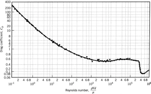
in an ideal potential flow, in which~u denotes direction of flow andθ is the angle on the cylinder. . . 40 3.3 Experimental drag coefficient values as a function of Reynold’s
number for a smooth infinitely long cylinder in unidirec-tional flow. . . 43 3.4 Values ofCd versus KC for a range of β values. . . 44
4.1 The volume fraction function α values within the compu-tational domain, evaluated using the VOF method. Blue areas indicate the air, red indicates water and the thin green line is the interface location. . . 58 4.2 Illustration of node and control volume location during
grid generation with the FV method. . . 60 4.3 Illustration of typical 3D control volume. . . 60 4.4 Illustration of simple quadrilateral 2D control volume, where
midpoint P, outward normal vectorn, and surface area∇S
are labelled . . . 63 4.5 Illustration of distance flow travels per time step,
depen-dent on the Courant number. . . 72 4.6 Procedure followed by the PIMPLE solver in OpenFOAM. 79 4.7 The procedure followed by theinterFoam solver in
Open-FOAM. . . 82 4.8 Case-set up diagram for interFoam simulation. Names in
bold indicate folders that contain the information specified in the diagram. . . 83 5.1 Vertex and control volume face numbering convention used
in blockMesh with the direction of ordering indicated by the arrows. . . 94 5.2 Mesh with monopile present, transition zone magnified . . 95 5.3 Patch names for simulation with a monopile. Top image
displays entire computational domain and bottom image shows a close-up of the cylinder. . . 96 5.4 Streamlines att = 15.5 s for (a) Re= 40 and (b) Re= 300. 98
5.5 Streamlines forRe = 3900 at (a) t = 5 s and (b) t = 50 s. 99 5.6 Mesh convergence test results: horizontal velocity time
series at elevation z = 0.4 m under regular waves, at T = 3.5 s and H = 0.084 m, where details of mesh 1, mesh 2, mesh 3 and mesh 4 are given in Table 5.3. . . 103 5.7 Computational domain with differing relaxation zone lengths.105 5.8 Water particle velocity profiles obtained for different ζ
-values in (5.3) indicating their effect on the wave absorp-tion within the damping zone . . . 106 5.9 Surface elevation profiles along domain length att∗= 5 for
different wave absorption conditions and varying values for
ζ in equation (5.3). . . 106 5.10 Comparison between numerical predictions and analytical
solutions of linear wave parameters for waves with period
T = 4 s. Figures illustrate time series predictions for (a) surface elevation, (b) pressure time series, (c) horizontal velocity component, (d) vertical velocity component. For each parameter in these figures, the subscript ∞ denotes the analytical linear wave solution and the subscript N represents the numerical simulation. . . 109
5.11 Comparison between numerical predictions and analytical solutions of linear wave parameters for waves with period
T = 6 s. Figures illustrate time series predictions for (a) surface elevation, (b) pressure time series, (c) horizontal velocity component, (d) vertical velocity component. For each parameter in these figures, the subscript ∞ denotes the analytical linear wave solution and the subscript N represents the numerical simulation. . . 110 5.12 Comparison between numerical predictions and analytical
solutions of linear wave parameters for waves with period
T = 8 s. Figures illustrate time series predictions for (a) surface elevation, (b) pressure time series, (c) horizontal velocity component, (d) vertical velocity component. For each parameter in these figures, the subscript ∞ denotes the analytical linear wave solution and the subscript N represents the numerical simulation. . . 111 5.13 Comparison between numerical predictions and analytical
solutions of linear wave parameters for waves with period
T = 10 s. Figures illustrate time series predictions for (a) surface elevation, (b) pressure time series, (c) horizontal velocity component, (d) vertical velocity component. For each parameter in these figures, the subscript ∞ denotes the analytical linear wave solution and the subscript N represents the numerical simulation. . . 112
5.14 Comparison between numerical solutions and analytical predictions of linear wave parameters for waves of period
T = 4 s. Figure (a) shows the time series for the analytical solution with no cylinder present η∞, numerical solution using slip cylinder wall conditionηSand the diffracted
sur-face elevation ηD. Figure (b) is the time series for wave
forces calculated with the Morison equation, FM,
numeri-cally predicted wave forces using a slip wall condition, FM,
and the analytically calculated wave force due to diffrac-tion, FD. . . 114
5.15 Comparison between numerical solutions and analytical predictions of linear wave parameters for waves of period
T = 6 s. Figure (a) shows the time series for (a) the analytical solution with no cylinder present η∞, numeri-cal solution using slip cylinder wall condition ηS and the
diffracted surface elevation ηD. Figure (b) is the time
se-ries for wave forces calculated with the Morison equation, FM, numerically predicted wave forces using a slip wall
condition, FM, and the analytically calculated wave force
5.16 Comparison between numerical solutions and analytical predictions of linear wave parameters for waves of period
T = 8 s. Figure (a) shows the time series for (a) the analytical solution with no cylinder present η∞, numeri-cal solution using slip cylinder wall condition ηS and the
diffracted surface elevation ηD. Figure (b) is the time
se-ries for wave forces calculated with the Morison equation, FM, numerically predicted wave forces using a slip wall
condition, FM, and the analytically calculated wave force
due to diffraction, FD. . . 115
5.17 Comparison between numerical solutions and analytical predictions of linear wave parameters for waves of period
T = 10 s. Figure (a) shows the time series for (a) the analytical solution with no cylinder present η∞, numeri-cal solution using slip cylinder wall condition ηS and the
diffracted surface elevation ηD. Figure (b) is the time
se-ries for wave forces calculated with the Morison equation, FM, numerically predicted wave forces using a slip wall
condition, FM, and the analytically calculated wave force
due to diffraction, FD. . . 116
6.1 Location of Teesside Offshore Wind Farm. Image provided by EDF Energy Renewables. . . 121 6.2 Datawell Waverider Wave Buoy (DWR MkIII). Image
from EDF Energy Renewables. . . 121
6.3 Predicted amplitude as a function of wave frequency cal-culated in OpenFOAMaN compared to the analytical
for-mulationaAN for (a) September 2015, (b) December 2015,
(c) March 2015 and (d) June 2016. . . 126 6.4 Autumn time series for (a) free surface elevation and (b)
associated wave spectrum. Subscripts raw, an, N represent values obtained from the in situ data set, analytical rep-resentation and numerically simulation respectively. Fig-ure (b) includes an additional numerical simulation, rep-resented by the subcaption N2, to demonstrate mesh con-vergence. . . 129 6.5 Winter time series for (a) free surface elevation and (b)
associated wave spectrum. Subscripts raw, an, N repre-sent values obtained from the in situ data set, analytical representation and numerically simulation respectively. . . 129 6.6 Spring time series for (a) free surface elevation and (b)
associated wave spectrum. Subscripts raw, an, N repre-sent values obtained from the in situ data set, analytical representation and numerically simulation respectively. . . 130 6.7 Summer time series for (a) free surface elevation and (b)
associated wave spectrum. Subscripts raw, an, N repre-sent values obtained from the in situ data set, analytical representation and numerically simulation respectively. . . 131 6.8 Location of numerical wave gauges. Results are presented
for data obtained from wg11, located at the rear stagnation point of the cylinder. . . 134
6.9 Paraview visualization of wave diffraction pattern showing wake formation in the vicinity of a large-diameter surface-piercing cylinder, representing a turbine monopile. Wave input is from the March 2016 data set. . . 135 6.10 Surface elevation wave spectral density functions for the
raw surface displacement data, Sη, diffracted wave
spec-trumSη,D, numerical wave spectrum with a slip boundary
condition, Sη,S, and the numerical wave spectrum using
a no-slip boundary condition, Sη,N. Figures display wave
spectrum data for (a) Autumn, (b) Winter, (c) Spring and (d) Summer. . . 137 6.11 Predicted horizontal and vertical velocity component
spec-tra for (a) Autumn, (b) Winter, (c) Spring and (d) Sum-mer at a site in the southern North Sea. Horizontal compo-nents are denoted bySu and vertical bySw. The subscript ∞ refers to the undisturbed velocity spectrum, D is the diffracted velocity spectrum, S is the numerical spectrum using the slip condition, andN is the numerical spectrum using the no-slip condition. . . 139 6.12 In-line force spectrum of wave during (a) Autumn, (b)
Winter, (c) Spring and (d) Summer at submerged cylinder height z = -1.5 m . . . 140 6.13 Total in-line wave force spectra for waves during (a)
Au-tumn, (b) Winter, (c) Spring and (d) Summer at Teesside Offshore Wind Farm in the southern North Sea. . . 142
6.14 Surface elevation wave spectral density functions using in-creased cell density in the wave direction for the raw sur-face displacement data,Sη, diffracted wave spectrumSη,D
and numerical wave spectrum with a slip boundary condi-tion, Sη,S. . . 145
6.15 Surface elevation wave spectral density functions with (a) minimum 8 cells per wave height and (b) minimum 16 cells per wave height for the raw surface displacement data,Sη,
diffracted wave spectrum Sη,D and numerical wave
List of Tables
4.1 Discretisation schemes used in a typical multiphase simu-lation using VOF . . . 85 5.1 Boundary conditions used for constant current past a
cylin-der . . . 97 5.2 Drag and lift coefficient values for each simulation,
speci-fied by the Reynolds numberRe . . . 99 5.3 Mesh Details . . . 103 5.4 Boundary Conditions . . . 104 5.5 Mesh details for each linear wave in a NWT case . . . 107 5.6 Mesh details for each linear waves past a cylinder . . . 113 5.7 Reand KC values for linear waves past a monopile . . . . 114 6.1 Total CPU hours for each simulation of the undisturbed
sea state . . . 127 6.2 Autumn Statistical Values - September 2015 . . . 128 6.3 Winter Statistical Values - December 2015 . . . 130 6.4 Spring Statistical Values - March 2016 . . . 130 6.5 Summer Statistical Values - June 2016 . . . 130 6.6 Significant wave heights for Teesside Farm covering all
sea-sons over the 2015-2016 year . . . 136
6.7 Non-dimensional parameter values for Teesside Farm cov-ering all seasons over the 2015-2016 year . . . 141 6.8 Peak spectral force values for Teesside Farm covering
sea-sons during the 2015-2016 year. Units are given in GN2
Nomenclature
α Scalar field fluid volume fraction
αR Relaxation zone scalar fluid volume fraction
αS,βS Constants required for Pierson-Moskowitz and JONSWAP
spec-trum formulation ¯
x Parameter in JONSWAP spectrum, equal to gx/u β Frequency parameter in oscillating flow
χR Location within the relaxation zone
∆t Time increment s
∆x Cell element length m
∆z Cell element height m
˙
u Horizontal acceleration component m/s2
˙
u∞,v˙∞,w˙∞ 3D irregular velocity components m/s2 Bessel function parameter, = 1 when m = 0 and 2 otherwise
η Location of free surface m
ηD Diffracted surface elevation m
η∞ Irregular surface elevation m
γ Peak enhancement factor Γξ Rate of diffusion of field ξ
ΓT Surface tension coefficient
κ Turbulent kinetic energy per unit mass
κα Surface curvature
λ Wavelength m
a Arbitrary vector of interest
d Vector connecting adjacent cell centres
g Vertical acceleration due to gravity m/s2
ST Strain rate tensor
u Flow velocity vector m/s
Up Velocity vector at centroid point P x Location within cell
xp Location of cell centroid point
µ Dynamic viscosity Pa.s
µT Dynamic eddy viscosity Pa.s
∇p Pressure gradient
ν Coefficient of kinematic viscosity m2
/s
ω Angular wave acceleration rad/s ωn n-th angular wave frequency component rad/Hz ωu Parameter needed in Borgman force spectrum
φ Wave potential m2
/s
φD Diffracted velocity potential m2/s
φI Incident velocity potential m
2
/s
φR Refracted velocity potential m
2
/s
∆∆∆ Orthogonal term in discretised diffusion term
κκκ Non-orthogonal corrector term Ψ Wave phase
ψn n-th randomly sampled phase value within the range 0≤ψ ≤2π
ρ Fluid density kg/m2
σ Spectral width parameter dependent on fn
σT Surface tension kg/s2
ση2 Variance of free surface elevation m2
τ Reynolds stress tensor
Θ Wave direction, measured positive anti-clockwise from midpoint
ξ0 Old value of ζ
ξn New value of ξ
ξt Value of ξ(t) at time t ξb Boundary value of ζ ξN Value of ξ(x) at point N ξP Value of ξ(x) at point P ζ Relaxaton zone value
ζf Face value of ζ a Wave amplitude m aN Function of u at point N aP Function of u at point P an n−th amplitude component m Cd Drag coefficient Cm Inertia coefficient Co Courant number D Cylinder diameter m
D(f, θ) Directional spectral function
df Frequency step size Hz
F Mass flux through the cell face
FD Diffracted force N
fd Morison drag force N
Fm Force calculated with the Morison equation N
fm Morison inertia force N
fn n-th frequency component Hz
fp Modal frequency Hz
Fs Sampling frequency Hz
fx Ratio of distance f N and P N fz Zero-crossing frequency
Fp,D Drag force due to in-line unsteady pressure gradient N Fp,L Lift force due to transverse unsteady pressure gradient N G(kR) Diffraction solution parameter
H Wave height m
h Mean water depth m
Hm(1) Hankel function of 1st kind, of order m
Hs Significant wave height m
HT(f) Transfer function
Hs,D Diffracted significant wave height m Jm Bessel function of 1st kind, of order m
k Wave number rad/m kn n-th component wave number rad/m KC Keulegan-Carpenter Number
l Submerged cylinder length m
Lx Computational domain length Ly Computational domain width m Bessel function order
m0 Zeroth moment m
m2 Second moment m2
N Number of sampling points
p Total wave pressure N/m
p∗ Pressure in excess of hydrostatic Pa
Q Any specific parameter value in the volume of fluid
qb Gradient on the bounary
R Cylinder radius m Re Reynolds number Su(f) u velocity spectrum m 2 /s3 Sw(f) w velocity spectrum m 2 /s3 Su˙(f) u acceleration spectrum m 2 /s4
Sw˙(f) w acceleration spectrum m2/s4 Sη,D Diffracted wave elevation spectrum m2 Hz Sη(f) Frequency spectrum of surface elevation m
2
/Hz
Sξξ Source term
SF,B Borgman force spectrum N
2
/Hz
SF,D Diffracted force spectrum N2 Hz SF,M Morison force spectrum N2 Hz
SSM Smoothed spectrum unit/Hz
T Wave period s
t Time s
t∗ Normalised time
Tp Modal period s
u Horizontal velocity component m/s uD Diffracted horizontal velocity component m/s u∞, v∞, w∞ 3D irregular velocity components m/s w Vertical velocity component m/s wD Diffracted vertical velocity component m/s x, y Cartesian planar wave directions, in-line and transverse
respec-tively m
Ym Bessel function of 2nd kind, of order m
z Location measured vertically upwards from mean water level m [ξ] Column vector of dependent variables
[A] Square matrix
[R] Column vector of source terms H(U) Matrix operator
S Outward pointing face area vector A.R. Cell aspect ratio
CV Control volume
A,B Constants required in general spectral calculation BBC Bottom boundary condition
CFD Computational fluid dynamics CPU Central processing unit
CTV Crew transfer vessel
DFSBC Dynamic free surface boundary condition DFT Abbreviation for Discrete Fourier Transform f Cell face
FD Finite difference FE Finite element
FIR Finite impulse response FV Finite volume
FVM Finite volume method HPC High-performance computer
ITTC International Towing Tank Conference
KFSBC Kinematics free surface boundary condition MA Moving average
MAC Marker-and-cell
MULES Multidimensional universal limiter for explicit solutions N Neighbour cell centroid point
NWT Numerical wave tank
O & M Operations & Maintenance P Owner cell centroid point PDE Partial differential equation
PISO Pressure implicit splitting operator RANS Reynolds averaged Navier-Stokes
SIMPLE Semi-implicit method for pressure linked equations SOV Service operations vessel
SWATH Small waterplane area twin hull
SWL Still Water Level VOF Volume of fluid WK Wiener-Khinchin
Chapter 1
Introduction
1.1
Introduction
One of the greatest challenges facing society today is how to reduce the negative environmental impact due to CO2emissions entering the Earth’s
atmosphere. Global efforts to reduce CO2 emissions necessitate a decline
in energy production by large coal and gas power plants, accompanied by increasing development of clean energy production methods. By June 2015, 164 countries had adopted some form of renewable energy target to decrease carbon emissions (Kieffer and Couture, 2015).The European Union, for example, has set a target that 20% of energy must be obtained through renewable sources by 2020 (Sawin et al., 2015).
The marine environment provides a promising portfolio of renewable energy sources for coastal populations, which have an average population density three times that of the average global density (Small and Nicholls, 2003). The fastest growing is offshore wind power. Not only did offshore wind power exhibit a 17% increase in the year from 2013 to 2014, up to ∼433 GW worldwide, but also wind power was found to be a larger supplier of new power generation than any other technology (Kieffer and
Couture, 2015). As of January 2016, more than 3,000 offshore wind turbines (3.4 GW) were connected to the European grid (Pineda, 2016), bringing the global total to 12 GW. Of the available global capacity, 91% of offshore wind power presently commercially available is in Europe and the remaining 9% is located mostly in China, Japan, and South Korea (GWEC, 2016). China has set an ambitious goal to produce 30 GW of offshore wind energy by 2020 (Hong and M¨oller, 2012). However, due to increasing costs and insufficient marine spatial planning, Hong and M¨oller (2012) estimate that only 1 GW out of the target of 5 GW wind turbine capacity has been achieved to date.
Noting that estimates vary widely, offshore wind power nonetheless has huge potential: Krewitt et al. (2009) assessed the net exploitable po-tential to be about 16,000 TWh per year by 2050 and Capps and Zender (2010) calculated the overall global value of offshore wind energy to be approximately 340,000 Twh per year. Notwithstanding the technical po-tential for offshore wind power, current cost estimates put the investment cost per kilowatt hour for offshore wind to be approximately three times the investment per kilowatt hour for onshore wind (Taylor et al., 2016).
1.1.1
Operations & Maintenance Overview
Safe access to offshore wind turbine monopiles, which may be located 30-50 km from the shore (or onshore base) and in water up to 30 m deep (Corbetta et al., 2014, Sperstad et al., 2014), is essential to reducing the total energy cost of offshore wind power. Maintenance difficulties can occur even for near-shore wind farms; it was estimated recently that, for a wind farm off the coast of Ireland, the turbines were only accessible for repairs for 50-75% of the year (Breton and Moe, 2009, van Bussel et al.,
2001). Additional costs are incurred by hiring repair workers and vessels to transport the workers to the turbines. Operations and maintenance (O&M) costs can account for 25-50% of total energy production costs (Kostecki, 2014, Dalgic et al., 2015a, Maples et al., 2013). It has been estimated that costs could decrease by as much as 35% (Taylor et al., 2016) by 2025 with continued technological improvements and improved turbine access methods.
The rapid development and construction of offshore wind farms has outpaced research and there is a lack of consensus on the best methods for access and maintenance (van Bussel et al., 2001, Baagøe-Engels and Stentoft, 2016, Browell et al., 2016). In the context of global offshore wind farm capacity, Dalgic et al. (2015a) report that access for repairs is only possible on average for 200 days of the year, and reduces in areas with harsher climates. Access is by helicopter, service operations vessel (SOV), or crew transfer vessel (CTV) (Nielsen and Sorensen, 2011, Scheu et al., 2012). Helicopters have the advantage that they are not affected by wave conditions, but cannot be used to transport bulky equipment and are limited by the number of personnel that can travel aboard. Ad-ditionally, helicopters have a hire cost that is at least five times greater than a CTV (Aukcland and Garlick, 2015). SOVs are useful for carrying heavy equipment and transporting a larger number of repair workers but again have the disadvantage over other access methods such as CTVs of increased cost.
The smaller CTVs, such as monohulls, catamarans or Small Water-plane Area Twin Hull (SWATH) type vessels, are more economical and account for 41% of the access methods used (Dalgic et al., 2015a). Ac-cording to the National Renewable Energy Laboratory (NREL) report on
the development of offshore wind by Maples et al. (2013), the estimated availability of CTVs is between 61%-95%. The same report advises that the O&M strategy with the greatest potential to increase availability of the turbines and decrease costs is to improve the crew transfer system for the CTVs. By improving this system, total O&M costs can be decreased by an estimated $24.8M per year while increasing the average availability to 93% (Maples et al., 2013).
The only limiting sea state factor for CTV access is typically that
Hs ≤ 1.5 m, where Hs is the significant wave height (Dalgic et al.,
2015a, Halvorsen-Weare et al., 2013). In general, the use of the sig-nificant wave height parameter as the main access criterion introduces additional uncertainty because Hs depends on in situ wind and wave
conditions and also on the near-wake of the turbine monopile (Sperstad et al., 2014). UsingHsas the sole limiting factor provides no information
on the modality of the sea state, which is subject to seasonal changes. These additional variables imply that the significant wave height alone may not provide sufficient information from which to determine the safety of the crew members and the stability of the CTV under operational con-ditions. Moreover, methods of determining Hs vary between wind farms
and no regulation appears to exist whereby Hs can be determined. A
survey conducted by Hoffman (2011) found a total of 49 different models were used by offshore wind energy companies for maintenance strategies.
1.1.2
Offshore Wind Turbine Access Method
Fixed monopile offshore wind turbines make up 80% of offshore wind turbine types (IEA, 2013). The remaining 20% are made up of founda-tion types such as a tripod or floating wind turbines. In order to access
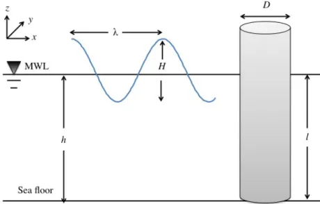
the turbine for repairs, the CTV is driven towards the turbine monopile and, under steady thrust from the engine, contact between the turbine transition piece and the CTV is maintained by frictional forces. Repre-sentative monopiles have a single turbine transition piece, ideally located downstream, into which the vessel is driven upwind and illustrated in figure 1.1. The CTVs in use are approximately 8-25 metres long and are manoeuvred to allow for the vessel fender to be in direct contact with the boat landing (Dalgic et al., 2015a). Note that figure 1.1 implies that the incident waves~u, are unidirectional, whilst in practice there is a like-lihood of multi-directional waves (see Section 2.3.1 and Chapter 7 for an in-depth discussion into wave directionality). The assumption of wave unidirectionality is made throughout this thesis.
Figure 1.1: Illustration of crew transfer system with CTV abutted against monopile
This benchmark problem has attracted previous interest in the con-text of fatigue-induced damage to the support column under wave loading (see e.g. Chen et al. (2014), Agarwal and Manuel (2011), Finnegan and Goggins (2012)). Only very limited research has considered the influ-ence of local hydrodynamics on CTV motion. No known experimental data exist concerning typical vessel motions during crew transfer; there are few research studies having considered the hydrodynamic forces on a floating body located within the wake of a fixed body, where frictional
forces instead of mooring lines are used to maintain contact.
Josse et al. (2011) presented a system in which hydrodynamic forces were ignored and the angle of the vessel against the turbine monopile was assumed to be the only parameter affecting the frictional contact. Al-though this approach was not validated, Josse et al. (2011) nevertheless found that wave frequency was a critical factor affecting motion and com-mented on the need for an improved hydrodynamic analysis of the effect of incident wave frequencies on vessel loading. K¨onig et al. (2017) also emphasised the necessity of calculating the hydrodynamic forces incident on the vessel and presented the results for two wave frequencies. This study found, as expected, that the influence of the monopile on the flow field decreases as the wave period increases. However, K¨onig et al. (2017) did not determine a limiting wave period for which the CTV could no longer operate. Moreover, this work focused primarily on the influence of the monopile in monochromatic wave fields in an experimental setting.
1.1.3
Turbine Access: Hydrodynamic limiting
Con-ditions
Changes in the near-wake flow field where the CTV lies can result in a weakening of the frictional force and CTV “slippage”, wherein the ves-sel becomes dislodged from the turbine monopile. When the CTV slips away from the monopile, crew members in transition are potentially en-dangered or there is a risk of incomplete maintenance leading to large economic losses. Eventually, it becomes necessary to predict the CTV motion under operating conditions, which requires detailed knowledge of the hydrodynamics and water particle kinematics within the vicinity of a turbine monopile. The hydrodynamic forces in the region, which are a
function of the incident wave period and monopile diameter, aid in iden-tifying the limiting conditions under which the vessel remains in contact with the monopile turbine. The limiting condition occurs when the total vertical hydrodynamic forces on the vessel overcome the frictional contact force between the vessel fender and the transition piece on the monopile turbine (K¨onig et al., 2017). When the frictional contact is overcome, the vessel is prone to slipping away from the turbine monopile.
Figure 1.2 presents screen shots from a video filmed from the vessel during crew transfer. The time stamp shows that figure 1.2a and figure 1.2f are only 30 seconds apart, but during this period the vessel is seen to slip away from the turbine and the repair worker is unable to move onto the vessel. Sea conditions in the video appear to show small-amplitude waves with no evidence of nonlinearity or large breaking waves. This implies that vessel slippage is due to the unobservable local hydrodynamic force incident on the vessel. Thus, an improvement here would be the determination of the local hydrodynamic force in an irregular sea state representing the conditions at an operational offshore wind farm.
1.2
Research Methods
The focus herein is on constructing an accurate representation of a spe-cific local sea state measured at an offshore wind farm and analysing the hydrodynamic response of the sea state interacting with a turbine monopile support column.
Predictions for the local hydrodynamic wave field are useful for engi-neers and vessel operators and common techniques for determining the wave field include both analytical and numerical methods. Analytical
(a) (b)
(c) (d)
(e) (f)
Figure 1.2: Images taken from a video documenting crew transfer between vessel and monopile. Video provided by Alexis Billet, Managing Director of Resilience Energy Consulting.
methods can be fast to solve and require minimal computational effort, but often neglect important hydrodynamic features such as nonlinearity or viscous effects. Numerical methods using computational fluid dynam-ics (CFD) are capable of resolving nonlinearities for more accurate flow field representations, but at a high computational overhead. Hence, this project aims to formulate both numerical and analytical methods capable of approximating the local wave field at a turbine monopile.
1.2.1
Analytical Wave Formulation
Wave motion, using linear wave theory, is first described for time-dependent monochromatic waves. Assuming that the principle of superposition ap-plies, waves in the open ocean are then represented as the sum of many periodic waves, each component with its own amplitude, frequency and phase. The wave amplitudes are acquired from a statistical analysis of the wave field in the frequency domain. Raw in situ data refers throughout to the time series of sea surface displacement, provided by EDF Energy Renewables from a single wave buoy located at Teesside Offshore Wind Farm. The in situ data is analysed and the local undisturbed sea state is formulated analytically.
Analytical methods are also applied to determine the total incident wave force on the monopile, in which the geometry is simplified by ne-glecting the transition piece. The monopile is modelled herein as a surface-piercing bottom-fixed circular cylinder in a regular, long-crested, small-amplitude wave field where the ratio of wave height to water depth is small and the waves are non-breaking. Hydrodynamic force loading is calculated typically depending on the wavelength-to-diameter ratio. Force calculation methods for both small- and large-diameter cylinders
are examined and the forces computed. For small-diameter cylinders, the Morison Equation (Morison et al., 1950) provides a good approximation for the wave loading in a viscous-dominant flow regime. The total linear diffraction force, derived by MacCamy and Fuchs (1954), provides a solu-tion for large-diameter cylinders when diffracsolu-tion effects occur and inertia forces are large. Wave force calculation methods are first presented for a monochromatic wave field, and then the formulation is extended to a unidirectional polychromatic wave field. In an irregular sea state, the wave force spectrum can be used to compare the forces in the frequency domain.
The wave field around the turbine monopile can also be determined analytically using the linear diffraction solution, again making the as-sumption that superposition applies in an irregular wave field. The time-dependent solution for the linear diffracted surface elevation val-ues is converted to the frequency domain for analysis, from which the diffracted wave amplitudes are obtained. As with the undisturbed sea state, the diffracted wave particle velocity components are derived from the diffracted amplitude spectrum. Once formulated, this solution is fast to compute and provides values of the local sea state at an offshore wind farm; conversion to the frequency domain can also give information on the modality of the wave field. In addition to providing values for an undisturbed sea state, the analytical method also provides satisfactory approximations of the interaction of the local sea state with a turbine monopile, and the wave kinematics within this region that would influ-ence vessel motion.
1.2.2
Numerical Methods
Numerical predictions are generated using the open-source CFD C++ library of solvers, OpenFOAM (version 2.4.0). OpenFOAM has been de-veloped by the CFD community to simulate many types of fluid flow, including multi-phase. OpenFOAM is employed here to simulate nu-merically the interaction between a cylinder representing the monopile support column and the local wave field.
The numerical model is validated for an undisturbed linear wave field, where waves are simulated with four different wave period values and a single wave height in a numerical wave tank. Following Feuchtwang and Infield (2012) and Dalgic et al. (2015b), the representative operating wave conditions are equivalent toHs ≤1.5 m in the vicinity of a support
column of diameter∼5 m. These values are chosen in order to model the type of conditions that prevail at a specific offshore wind site, Teesside Offshore Wind Farm off the east coast of the United Kingdom, where the key wave periods are in the range 4 s ≤ T ≤ 10 s and the mean water depth h ≈15 m.
The analytically calculated wave force incident on the cylinder for a regular wave field, where well-documented solutions for the force loading exist, allows the numerical model to be verified in a regular wave field. Altering the wave period also means that the wavelength-to-diameter ra-tio changes and the effect on the flow due to the presence of the monopile becomes more apparent with decreasing wavelength. Diffraction and viscous solutions for the force calculation are employed and compared to numerical solutions, through application of no-slip and slip cylinder wall boundary conditions that coincide with viscous- or inertia-dominant
regimes.
Finally, following verification of the numerical model against the an-alytical solutions for regular waves, the model is extended to incorporate an irregular wave field using statistical analysis of in situ data tracking the ocean surface. To accomplish this, the in situ displacement data must be converted to the frequency domain, from which important sta-tistical parameters, such as the significant wave height and modal wave period, can be determined from the spectrum. Additionally, although the assumption is made throughout that the wave field is unidirectional, a statistical representation of the displacement data can provide infor-mation on the modality of the wave spectra.
To simulate the irregular wave field numerically, a boundary condition is developed for the purpose of this research for use with OpenFOAM. The boundary condition is capable of generating a specific sea state, de-pendent on the spectral values (see Section 2.3). Simulating the exact sea state at an offshore wind farm provides a method with which the interaction of a specific sea state with a turbine monopile may be de-termined numerically. OpenFOAM is a fully nonlinear model and can resolve higher-order effects neglected by the linear methods.
The work undertaken for this thesis has produced two methods for de-termining the detailed linear wave kinematics found locally at an offshore wind farm, based on data obtained from the location. With knowledge of the wake kinematics within this region and the measured sea state found at an offshore wind farm, practitioners can decide whether to at-tempt turbine access with much greater detail of the hydrodynamics, in addition to knowledge of the significant wave height.
1.3
Purpose of Research
The purpose of this thesis is to provide operators of companies employing offshore wind turbine repair workers, and engineers tasked with improv-ing the O&M process, a method of resolvimprov-ing the sea state at specific offshore wind farms. Current repair vessel access limits rely solely on the significant wave height, an observable parameter which provides no infor-mation on the directionality of a sea state. Access methods, in which the vessel operator manoeuvres the vessel into the turbine and continuously runs the vessel motor, thereby driving the vessel into the turbine and relying on frictional contact, cannot account for hydrodynamics within the wave field or non-negligible wave diffraction.
By computing both numerical and analytical solutions to the wave-monopile interaction, it can be shown that the analytical linear diffraction solution for irregular waves provides a good approximation to the wave field in the vicinity of a turbine monopile, when compared to the fully nonlinear numerical solution. Analytical solutions are beneficial to engi-neers or consultants who do not have access to large supercomputers or significant computational resources.
The results provided by the current analytical method can give prac-titioners a good initial approximation of the wave field that a CTV will enter. When available, improved results for the wave field can be pro-vided through numerical methods capable of resolving nonlinearities. The open-source numerical method used here is freely available, making it an affordable option for engineers or consultants without access to powerful computers with multi-core processors. By developing the boundary con-dition for generating any unidirectional wave field from a given spectral
data set, many additional numerical simulations of the interaction of an actual sea state with offshore structures can be examined.
Both analytical and numerical calculation methods are employed to present two sets of solutions for the local hydrodynamic wave field. Each solution method has advantages and disadvantages. The analytical so-lution has the advantage that it can produce approximate results of the wave kinematics around a monopile quickly, but is restricted to linear so-lutions of an inviscid flow. The numerical solution has the advantage that it can resolve nonlinearities and other complicating flow factors, with the obvious drawback of a large computational overhead. Nevertheless, both methods utilise field information obtained as wave buoy data and lead to sensible approximations of the local wave field.
1.4
Aim and Objective
The aim of this thesis is to provide offshore wind farm practitioners with a method for determining the sea state at an offshore wind farm, the wave loading on a turbine monopile and the accompanying local hydro-dynamics. This thesis describes the following steps:
1. A statistical analysis of the spectral distribution of the surface el-evation from data obtained from an in situ wave buoy measuring surface displacement at Teesside Offshore Wind Farm in the south-ern North Sea.
2. Utilisation of the verified spectral distribution values as input, to formulate the undisturbed surface elevation and wave particle kine-matics analytically.
3. Reproduction of the sea state numerically through application of a boundary condition developed for this project. This boundary condition, developed for use with OpenFOAM, allows for the cal-culation of in-line and horizontal velocity values on the boundary of the computational domain from spectral values.
4. Formulation of analytical solutions for the spectrum of wave forces on the turbine monopile in the irregular sea state represented by the wave buoy data. The solution methods reflect the influence that the presence of the monopile has on the passing wave field. For shorter wave periods, wave diffraction is expected to occur, thereby affecting the local hydrodynamics.
5. Employ application of linear wave diffraction solutions in an irregu-lar sea to calculate the diffracted surface elevation and its spectrum. Obtain the diffracted significant wave height and local diffracted hydrodynamics relevant to vessel motion, such as velocities, ac-celerations, and forces, analytically in the vicinity of the turbine monopile.
6. Examine numerically the interaction between the simulated sea state and the turbine monopile; compare and contrast wave forces and diffracted hydrodynamics to solutions obtained analytically.
1.5
Thesis Outline
Chapter 2 describes the analytical formulation of a linear wave field, in which wave motion in a regular wave field is first discussed, followed by the statistical formulation used for the sea state in the open ocean.
Chapter 3 examines wave loading on a cylinder in unidirectional and in oscillating flow, together with the spectral representation of forces on a cylinder in irregular waves. Chapter 4 considers the numerical model, meshing and discretisation methods, and solution algorithms used in OpenFOAM. Chapter 5 describes the preliminary tests, including the in-teraction between a steady current and a surface-piercing cylinder; linear progressive wave loading on a cylinder is also considered. This chapter also discusses simulation of an undisturbed regular wave field and the interaction between the regular wave field and surface-piercing cylinder. Details are given of an investigation into the effect that the wave absorp-tion zone has on the computaabsorp-tional domain length, and whether the ab-sorption zone length can be reduced through an adjustment of relaxation zone parameters. Chapter 6 describes an extension of the regular wave model to represent an irregular wave field based on wave buoy data from Teesside Offshore Wind Farm during each of the four seasons throughout 2015/2016. From thisin situ data, the analytical and numerical methods outlined in the previous chapters are applied to generate the sea state at Teesside offshore wind farm and calculate the interaction between the local sea state and a wind turbine monopile. Chapter 7 summarises the overall conclusions, challenges and suggestions for future work.
Chapter 2
Mathematical Theory
Chapter Summary
The mathematical theory presented in this chapter focuses on determin-ing the water particle kinematics in an undisturbed wave field. Wave motions are described for regular linear waves and for an irregular wave field. Statistical methods are outlined for determining the water particle amplitudes, velocities and accelerations in an irregular wave field. A brief discussion of wave directionality is also provided.
2.1
Introduction
An analytical approximation to the wave particle kinematics around an offshore wind turbine support column can provide important information about the waves incident on a CTV under operating conditions. The undisturbed wave field far from the monopile is modelled using linear wave theory for small-amplitude long-crested waves; a brief discussion of linear wave theory is given in Section 2.2. In the ocean, where waves of many different frequencies and amplitudes contribute to the wave field,
the undisturbed sea state is often described by the superposition of linear sinusoidal waves (Faltinsen, 1990). It is usually assumed in linear theory that the waves are long-crested and of small-amplitude, with the fluid incompressible and inviscid and the flow is irrotational.
As a consequence of the irregular properties of the ocean sea state, a statistical spectral representation of the wave elevation in the frequency domain can also be used to approximate the entire wave field and provide summary statistics. The undisturbed wave amplitudes and water particle kinematics incident on the turbine monopile are computed from the wave elevation spectrum (Sarpkaya, 1986). For engineering applications, it is usual that wave displacement data is obtained from in situ wave buoys, which in this case are located at the relevant wind farm. Statistical rep-resentations of the wave buoy displacement data can be used to model the sea state and verify that the correct sea state has been produced. Further details describing sea state representation are given in Section 2.3. Treatment of waves in a multidirectional sea state is briefly consid-ered in Section 2.3.1, although this thesis will restrict the later analysis to unidirectional waves.
2.2
Linear Wave Theory
Typically, CTV access to a turbine monopile is limited by the significant wave height Hs, which for most vessels currently in use must be below
1.5 m for operation (Dalgic et al., 2015a, Halvorsen-Weare et al., 2013). At the site of interest herein, Teesside Offshore Wind Farm, the average water depth is 15 m. For the small-amplitude waves required for CTV access, it can be assumed that for all relevant wave fields, the operating
wave height-to-depth ratio is ≤0.1.
Assuming that the fluid is incompressible and inviscid, with the mo-tion irrotamo-tional, a velocity potential φ may be employed, which satisfies Laplace’s equation ∇2φ= 0, (2.1) in which ∇=i ∂ ∂x +j ∂ ∂y +k ∂ ∂z, (2.2)
wherexandyare Cartesian distance components in the horizontal plane and z the vertical distance measured vertically upward from the still water level. Figure 2.1 illustrates the wave direction and other parameters defining the wave field and cylinder properties.
Figure 2.1: Diagram indicating the wave parameters for a linear wave moving past a cylinder
It is assumed that the waves are regular and long-crested with
plitude a. Boundary conditions on the bottom and at the free surface must be applied to determine the velocity potentialφthat satisfies (2.1). On the bottom, located at z =−h, where h is the water depth, no flow should pass through the boundary and the bottom boundary condition (BBC) is ∂φ ∂z z=−h = 0. (2.3)
Bernoulli’s equation for unsteady flow is then used to determine the pres-sure condition on the free-surface. The unsteady Bernoulli equation pro-vides the dynamic free-surface boundary condition (DFSBC), given by
1 2(u 2 +v2+w2) + p ρ +gz+ ∂φ ∂t = 0, (2.4)
where u, v and w are the velocity components, g is acceleration due to gravity, p is the dynamic pressure, ρ is the fluid density and t is time. Assuming thatu2,v2 andw2 are small, the linearised form of the DFSBC is given by ∂φ ∂t +gη z=η = 0, (2.5)
where η is the free-surface elevation above the still water level. From the boundary conditions above, the solution of (2.1) is given by (see e.g. Dean and Dalrymple (1991))
φ=−aω
k
coshk(h+z)
coshkh sinΨ (2.6)
where k= (k1, k2,0) is the wavenumber vector, k =|k| is the
given as a function of position vectorx and time t as
Ψ(x, t) = (k.x−ωt), (2.7) where ω is the frequency in radians/sec. The linearised kinematic free surface boundary condition (KFSBC) ensures that the vertical velocity component is equal to the rate of displacement of the free surface, such that ∂φ ∂z z=0 = ∂η ∂t. (2.8)
The value for η when no cylinder is present can be given as a sinusoidal motion of constant amplitude a = H/2, where H is the wave height, given by
η=acos (k.x−ωt). (2.9) From (2.8) and (2.9), k (where the subscript 1 has been dropped for simplicity) is related to ω by the linear dispersion relation,
ω2 =gktanhkh, (2.10) in which g is acceleration due to gravity. The linear dispersion rela-tion describes the change in wave properties with respect to physical parameters; the wavelengths become shorter and the speed is decreased with increasing depth and constant wave period (Sarpkaya and Isaacson, 1981). The wave period T and wave length λ are related to ω and k, respectively, by
ω= 2π
T (2.11)
and
k = 2π
λ . (2.12)
The system is considered to be linear if it satisfies properties of scaling and superposition. Equation (2.10) is usually solved iteratively using a standard technique, such as the Newton-Raphson method or bi-section.
The water particle velocity components in the horizontal x and y
directions and verticalz are obtained directly from the velocity potential as u= ∂φ ∂x, v = ∂φ ∂y, w = ∂φ ∂z. (2.13)
Similarly, the water particle accelerations are defined as
˙ u= Du Dt, v˙ = Du Dt, w˙ = Du Dt. (2.14)
From (2.6) and (2.13) and by applying the linear dispersion relation (2.10), the undisturbed in-line and vertical velocity components in a reg-ular wave field can be written
u= H
2
gk ω
coshk(h+z)
cosh(kh) cos ΨcosΘ (2.15)
v = H
2
gk ω
coshk(h+z)
cosh(kh) cos ΨsinΘ (2.16)
w= H 2 gk ω sinhk(h+z) coshkh sin Ψ (2.17)
and similarly the accelerations can be written as ˙ u= Du Dt =− H 2gk coshk(h+z)
sinhkh sin Ψ cos Θ (2.18)
˙ v = Dv Dt =− H 2gk coshk(h+z)
sinhkh cos Ψ sin Θ (2.19)
˙ w= Dw Dt = H 2gk sinhk(h+z) sinhkh cos Ψ. (2.20)
By applying the linearised form of the Bernoulli equation from (2.5), the pressure underneath a progressive wave, written in terms of the po-tential, is
p=−ρ∂φ
∂t −ρgz. (2.21)
In (2.21), the first term on the right-hand-side describes the dynamic pressure component due to the motion of the fluid and the second term is the hydrostatic component from gravity, acting in the −z direction. The static pressure is a function of depth only and does not contribute to the time-dependent loading. Only waves in a regular wave field with a single wave frequency have been considered thus far. Extension to an irregular wave field with multiple wave frequencies will be discussed in Section 2.3. Henceforth, the wave formulation will be given for a 2-D wave field, where the angle of approach Θ = 0.
2.3
Ocean Statistics
For small-amplitude waves, the unidirectional sea state can be repre-sented as the linear superposition of waves with a range of frequencies and amplitudes where the random phasing ψ is between 0 and 2π and
represents the random distribution of wave phases inherent in an irregu-lar sea. In the ocean, it is common to define the stationary sea state in the frequency domain by its spectral functionS(f) (Dean and Dalrymple, 1991), wheref is frequency in Hz andf =ω/2π.
To compute the wave spectrum, a Fourier analysis of the wave field is conducted. Fourier analysis permits any continuous or piecewise-continuous function to be represented in the time domain as the sum of periodic functions with varying frequencies and Fourier coefficients, cor-responding to the individual wave amplitudes (Sarpkaya and Isaacson, 1981). For the greatest accuracy, the wave field is ideally extracted from multiple wave buoys contemporaneously measuring surface displacement over a prolonged length of time (McAllister et al., 2017). Whilst a Fourier transform can be computationally demanding and time-consuming to cal-culate, a Fast Fourier Transform (FFT) is an algorithm that can very quickly compute a Discrete Fourier Transform (DFT), which converts a finite sequence of samples of a function into same-length equidistant discrete samples. The spectral function is then related to the FFT by
S(f) = 1
FsN
|FFT|2, (2.22)
where Fs is the sampling frequency and N is the total number of
fre-quency bins.
It can be difficult to obtain displacement data from a specific location and it is common to apply established wave spectra when the relevant data are not available. Wave spectra are depth- and location-dependent and a number of models have been developed to describe the charac-teristics of a wave spectrum for key parameters including wave period,
wind direction and fetch; the fetch determines whether the sea state is fully developed or not. Spectral equations for wave spectra measured at a specified point are typically of the form
S(f) = A f5e −B f4 , (2.23)
where A and B are constants that represent parameters needed for cal-culating the spectral values.
The key parameters and representative wave spectrum are location-dependent. Common wave parameters are the significant wave height
Hs, which is an observational measurement of the average of the highest
one-third of all waves, and the mean wave periodTp (Chakrabarti, 1987).
For fully-developed unidirectional seas, the Pierson-Moskowitz Spectrum is often applied. The single-sided Pierson-Moskowitz spectrum is formu-lated from either one (spectral wave height or windspeed or peak period) or two (significant wave height and peak parameter) known parameters (Pierson and Moskowitz, 1964). The Pierson-Moskowitz Spectrum, de-fined from zero to infinity, is given by
S(f) = 1 (2π)4αsg 2 f−5e −βs(fpf )4 , (2.24)
where αs = 0.0081 and βs = 0.74 are empirically determined numerical
constants controlling the intensity and shape of the spectra, respectively, and peak frequency fp = 2π1 0.4
p
g/Hs (Pierson and Moskowitz, 1964).
The Pierson-Moskowitz Spectrum was originally the recommended spec-tral formation by the International Towing Tank Conference (ITTC), but due to its dependence on fully developed seas, two-parameter spectra such as the JONSWAP spectrum was developed for the North Sea, where the
fetch length is limited by land (Hasselmann et al., 1973). The JONSWAP spectrum is a fetch-limited variation of the Pierson-Moskowitz spectrum defined by S(f) = 1 (2π)4αsg 2f−5e −5 4 f fp −4 γδ , (2.25)
where γ is the peak enhancement factor with a given value of 3.3 and
δ= exp −(f−fp) 2 2σ2f2 p , (2.26) αs= 0.076¯x−0.22, (2.27) ¯ x= gx U2, and (2.28) σ= 0.7 for f ≤fp 0.9 for f > fp. (2.29)
The value ¯x indicates fetch where U is the wind speed taken at 19.5 m above sea level. The JONSWAP spectrum is valid for seas that are narrow-banded (such as the North Sea) and is often used in the offshore industry. Other spectral types, such as the modified Pierson-Moskowitz spectrum (Bretschneider spectrum) (Bretschneider, 1959), have been de-veloped for seas with different parameters, locations, currents, fetch, etc. For any wave spectrum, the area under the spectral curve is the zeroth moment,m0, about the axis (Pierson and Moskowitz, 1964), and gives the
total energy within the spectral function. The value for m0 is equivalent
to the variance of the wave elevation time series ση2 (Chakrabarti, 1987), or
σ2η =m0 =
Z ∞
0
S(f)ηdf. (2.30)
From the frequency spectrum, the significant wave height Hs and
am-plitude components an can be found from (Papoulis, 1991, Sumer and
Fredsøe, 2006) to be Hs = 4 √ m0 (2.31) and an = q 2S(f)η∆f . (2.32)
Under the assumption that superposition applies, the undisturbed free surface elevation of a two-dimensional random sea state in the (x, z )-plane is described by linear wave theory and the wave spectrum (2.22) (Dean and Dalrymple, 1991). For an irregular wave (2.9) becomes
η∞=
N X
n=1
ancos(knx−ωnt+ψn), (2.33)
where the amplitude of the n-th component an is obtained from (2.32)
andψ is randomly sampled from the phase distribution. Equation (2.33) is the 2-D representation whenycomponents are small, which is assumed henceforth. The linear dispersion relation for this frequency component is given by wn2 =gkntanhknh. Similarly by superposition, the undisturbed
vertical and horizontal velocity components in irregular waves may be expressed
u∞ = N X n=1 anωn coshkn(z+h) coshknh cos (knx−ωnt+ψn) cos Θ (2.34) w∞ = N X n=1 anωn sinhkn(z+h) coshknh sin (knx−ωnt+ψn), (2.35)
and the irregular water particle acceleration components are
˙ u∞= Du∞ Dt = N X n=1 angkn coshkn(h+z) sinhknh sin(knx−ωnt+ψn) cos Θ (2.36) ˙ w∞= Dw∞ Dt = N X n=1 angkn sinhkn(h+z) sinhknh cos(knx−ωnt+ψn). (2.37)
The analytically calculated undisturbed surface elevation in (2.33) can be statistically correlated to the in situ displacement data by evaluating the wave spectrumS(f)η of both data sets and comparing them0 values
and spectral shapes. Equation (2.30) can be used to verify that each wave spectrum correctly corresponds to its respective surface elevation data.
The average frequency that the signal crosses thex-axis in the upward direction, or the zero-crossing frequency, can also be obtained from the wave spectrum, fz = r m2 m0 , (2.38)
where m2 is the second moment, given by
m2 =
Z ∞