Department of Econometrics and Business Statistics
http://www.buseco.monash.edu.au/depts/ebs/pubs/wpapers/Coherent mortality forecasting:
the product-ratio method with
functional time series models
Rob J Hyndman, Heather Booth and Farah Yasmeen
February 2011
product-ratio method with
functional time series models
Rob J Hyndman
Department of Econometrics and Business Statistics, Monash University, VIC 3800
Australia.
Email: [email protected]
Heather Booth
Australian Demographic and Social Research Institute The Australian National University
Australia.
Email: [email protected]
Farah Yasmeen
Department of Econometrics and Business Statistics, Monash University, VIC 3800
Australia.
Email: [email protected]
product-ratio method with
functional time series models
AbstractWhen independence is assumed, forecasts of mortality for subpopulations are almost always divergent in the long term. We propose a method for non-divergent or coherent forecasting of mortality rates for two or more subpopulations, based on functional principal components models of simple and interpretable functions of rates. The product-ratio functional forecasting method models and forecasts the geometric mean of subpopulation rates and the ratio of subpopulation rates to product rates. Coherence is imposed by constraining the forecast ratio function through stationary time series models. The method is applied to sex-specific data for Sweden and state-specific data for Australia. Based on out-of-sample forecasts, the coherent forecasts are at least as accurate in overall terms as comparable independent forecasts, and forecast accuracy is homogenised across subpopulations.
Keywords:Mortality forecasting, coherent forecasts, functional data, Lee-Carter method, life expectancy, mortality, age pattern of mortality, sex-ratio.
1
Introduction
In recent years, we have seen considerable development in the modeling and forecasting of mortality rates. This includes the pioneering work byLee and Carter (1992) and a variety of extensions and modifications of the single-factor Lee-Carter model (for example,Lee and Miller 2001a,Booth et al. 2002a,Currie et al. 2004,Renshaw and Haberman 2003,Cairns et al. 2006, 2008, Hyndman and Ullah 2007); Booth and Tickle (2008) provide a comprehensive review. Most of this work on mortality forecasting has focused on forecasting mortality rates for a single population. However, it is often important to model mortality for two or more populations simultaneously, as for example, when forecasting mortality rates by sex, by states within a country, or by country within a larger region such as Europe. In such cases, it is usually desirable that the forecast rates do not become divergent over time.
Non-divergent forecasts for sub-populations within a larger population have been labelled “coherent” (Li and Lee 2005). Coherent forecasting seeks to ensure that the forecasts for related populations maintain certain structural relationships based on extensive historic observation; for example that male mortality remains higher by an “acceptable” margin than female mortality, or that the forecasts for similar countries, or regions within the same country, do not diverge radically. The problem of obtaining coherent forecasts has previously been considered byLee and Nault(1993),Lee(2000) andLi and Lee(2005) in the context of the Lee-Carter model.Lee
(2006) presents a general framework for forecasting life expectancy as the sum of a common trend and the population-specific rate of convergence towards that trend.
A related problem occurs in the case of disaggregated forecasts where there are several additive absorbing states; for example, in forecasting mortality by cause of death. Wilmoth (1995) quantified the way in which the multiple-decrement forecast based on proportional changes in mortality rates by cause of death tends to be more pessimistic than the single-decrement forecast of total rates. Using death densities and compositional methods,Oeppen(2008) found that the multiple-decrement compositional forecast is not always more pessimistic than the single-decrement case.
In Section 2, we propose a new method for coherent mortality forecasting which involves
forecasting interpretable product and ratio functions of rates using the functional data paradigm introduced inHyndman and Ullah(2007). The product-ratio functional forecasting method can be applied to two or more sub-populations, incorporates convenient calculation of prediction
modelling framework such asHyndman and Booth(2008). The new method is simple to apply, flexible in its dynamics, and produces forecasts that are at least as accurate in overall terms as the comparable independent method.
In Section 3, we illustrate the product-ratio method with functional time series models by applying it to Swedish male and female mortality data and Australian state-specific mortality data. We compare our mortality forecasts with those obtained from independent functional time series models, and evaluate relative accuracy through out-of-sample forecasts. Section4
contains a discussion of the method and findings.
2
A coherent functional method
We initially frame the problem in terms of forecasting male and female mortality rates, as the two-sex application is the most common and the best understood. However, our method can be applied generally to any number of subpopulations.
Letmt,F(x) denote the female death rate for agexand yeart,t= 1, . . . , n. We will model the log death rate,yt,F(x) = log[mt,F(x)]. Similar notation applies for males.
2.1 Functional data models
In the functional data paradigm, we assume that there is an underlying smooth functionft,F(x)
that we are observing with error. Thus,
yt,F(xi) = log[ft,F(xi)] +σt,F(xi)εt,F,i, (1)
where xi is the centre of age-group i (i = 1, . . . , p), εt,F,i is an independent and identically
distributed standard normal random variable andσt,F(xi) allows the amount of noise to vary with agex. Analogous notation is used for males. For smoothing, we use weighted penalized regression splines (Wood 1994) constrained so that each curve is monotonically increasing above agex= 65 (seeHyndman and Ullah 2007).
2.2 Product-ratio method for males and females
We define the square roots of the products and ratios of the smoothed rates for each sex:
pt(x) =
q
ft,M(x)ft,F(x) and rt(x) =
q
We model these quantities rather than the original sex-specific mortality rates. The advantage of this approach is that the product and ratio will behave roughly independently of each other. On the log-scale, these are sums and differences which are approximately uncorrelated (Tukey 1977).
We use functional time series models (Hyndman and Ullah 2007) forpt(x) andrt(x):
log[pt(x)] =µp(x) + K X k=1 βt,kφk(x) +et(x) (2a) log[rt(x)] =µr(x) + L X `=1 γt,`ψ`(x) +wt(x), (2b)
where the functions{φk(x)}and{ψ`(x)}are the principal components obtained from
decompos-ing{pt(x)}and{rt(x)}respectively, andβt,kandγt,` are the corresponding principal component
scores. The functionµp(x) is the mean of the set of curves{pt(x)}, andµr(x) is the mean of{rt(x)}.
The error terms, given byet(x) andwt(x), have zero mean and are serially uncorrelated.
The coefficients, {βt,1, . . . , βt,K} and{γt,1, . . . , γt,L}, are forecast using time series models as
de-tailed in Section2.4. To ensure the forecasts are coherent, and do not diverge, we require the coefficients{γt,`} to be stationary processes. The forecast coefficients are then multiplied by
the basis functions, resulting in forecasts of the curvespt(x) andrt(x) for futuret. Ifpn+h|n(x)
and rn+h|n(x) are h-step forecasts of the product and ratio functions respectively, then fore-casts of the sex-specific mortality rates are obtained usingfn+h|n,M(x) =pn+h|n(x)rn+h|n(x) and
fn+h|n,F(x) =pn+h|n(x)/rn+h|n(x).
2.3 Product-ratio method for more than two subpopulations
More generally, suppose we wish to apply a coherent functional method forJ >2 subpopulations. Let pt(x) = h ft,1(x)ft,2(x)· · ·ft,J(x) i1/J (3) and rt,j(x) =ft,j(x)/pt(x), (4)
wherej= 1, . . . , J andpt(x) is the geometric mean of the smoothed rates and so represents the
joint (non-stationary) behaviour of all subpopulations. The previous equations for males and females are a special case of these equations whenJ= 2.
We can assume approximate independence between the product functionspt(x) and each set of ratio functionsrt,j(x). The ratio functions will satisfy the constraintrt,1(x)rt,2(x)· · ·rt,J(x) = 1.
We use functional time series models forpt(x) and eachrt,j(x) forj= 1,2, . . . , J:
log[pt(x)] =µp(x) + K X k=1 βt,kφk(x) +et(x) (5a) log[rt,j(x)] =µr,j(x) + L X l=1 γt,l,jψl,j(x) +wt,j(x). (5b)
It is only necessary to fitJ−1 models for the ratio functions due to the constraint — recall that
we only needed one ratio model for the two-sex case whenJ= 2. However, fitting allJ models will simplify the variance calculation for producing prediction intervals.
Thus, the implied model for each group is given by
log[ft,j(x)] = log[pt(x)rt,j(x)] =µj(x) + K X k=1 βt,kφk(x) + L X `=1 γt,`,jψ`,j(x) +zt,j(x), (6)
whereµj(x) =µp(x) +µr,j(x) is the group mean andzt,j(x) =et(x) +wt,j(x) is the error term. Note
that equation (6) is equivalent to equation (15) inHyndman and Ullah(2007). Here, we are providing an easy and interpretable approach to estimation for this model.
2.4 Forecasts and prediction intervals
Forecasts are obtained by forecasting each coefficientβt,1, . . . , βt,K andγt,1, . . . , γt,Lindependently.
There is no need to consider vector models as theβt,k coefficients are all uncorrelated by
con-struction (seeHyndman and Ullah 2007), as are theγt,`coefficients. They are also approximately
uncorrelated with each other due to the use of products and ratios.
The coefficients of the product model,{βt,1, . . . , βt,K}, are forecast using possibly non-stationary
ARIMA models (Shumway and Stoffer 2006) without restriction. When fitting ARIMA models,
we use the automatic model selection algorithm given byHyndman and Khandakar(2008) to
select the appropriate model orders.
The coefficients of the ratio model,{γt,1,j, γt,2,j, . . . , γt,L,j},j= 1,2, . . . , J, are each forecast using
any stationary ARMA(p, q) (Box et al. 2008) or ARFIMA(p, d, q) process (Granger and Joyeux 1980,Hosking 1981). The stationarity requirement ensures that the forecasts do not diverge, or are coherent. We have found ARFIMA models useful for forecasting the ratio function
coefficients as they provide for longer-memory behaviour than is possible with ARMA models. In implementing ARFIMA(p, d, q) models, we estimate the fractional differencing parameter
d using the method of Haslett and Raftery(1989), we use the algorithm of Hyndman and
Khandakar(2008) to choose the orderspandq, then we use maximum likelihood estimation (Haslett and Raftery 1989) and the forecast equations of Peiris and Perera (1988). In the stationary ARFIMA models,−0.5< d <0.5; ford= 0, an ARFIMA(p, d, q) model is equivalent to
an ARMA(p, q) model.
Let ˆβn+h|n,k denote theh-step ahead forecast ofβn+h,kand let ˆγn+h|n,`,j denote theh-step ahead forecast ofγn+h,`,j. Then theh-step ahead forecast of logmn+h,j(x) is given by
log[ ˆmn+h|n,j(x)] = ˆµj(x) + K X k=1 ˆ βn+h|n,kφk(x) + L X `=1 ˆ γn+h|n,`,jψ`,j(x). (7)
Because all terms are uncorrelated, we can simply add the variances together so that
Varnlog[mn+h,j(x)]| In o = ˆσµ2j(x) + K X k=1 un+h|n,kφk2(x) + L X `=1 vn+h|n,`,jψ2`,j(x) +se(x) +sw,j(x) +σn2+h,j(x), (8) whereI
n denotes all observed data up to timenplus the basis functions{φk(x)}and{ψ`(x)},
un+h|n,k= Var(βn+h,k|β1,k, . . . , βn,k) andvn+h|n,k= Var(γn+h,k|γ1,k, . . . , γn,k) can be obtained from the time series models, ˆσµ2j(x) (the variances of the smoothed means) can be obtained from the smoothing method used,σt,j2(x) is given byHyndman and Booth(2008),se(x) is estimated by
averaging ˆet2(x) for eachxandsw,j(x) is estimated by averaging ˆwt,j2 (x) for eachx. A prediction interval is then easily constructed under the assumption that the errors are normally distributed. Life expectancy forecasts are obtained from the forecast mortality rates using standard life table methods (Preston et al. 2001). To obtain prediction intervals for life expectancies, we simulate a large number of future mortality rates as described inHyndman and Booth(2008) and obtain the life expectancy for each. Then the prediction intervals are constructed from percentiles of these simulated life expectancies.
3
Empirical Studies
In this section, we will illustrate the product-ratio functional forecasting method using two applications: male and female data for Sweden, and state data for Australia. With each ap-plication, we compare the forecast accuracy of our method with the accuracy of independent functional forecasts for each subpopulation, based on out-of-sample forecasts. This does not, of course, assess the accuracy of our forecasting applications, but it does provide two comparisons of the accuracy of the coherent and independent approaches. We fit each model to the firstt observations and then forecast the mortality rates for the observations in yearst+ 1, t+ 2, . . . , n. The value oftis allowed to vary fromn1= 20 ton−1. Correspondingly, the forecast horizon
varies fromn−20 to 1.
For thejth group and forecast horizonh, we define the mean square forecast error (MSFE) to be
MSFEj(h) = 1 (n−h−n1+ 1)p n−h X t=n1 p X i=1 n log[mt+h,j(xi)]−log[ ˆmt+h|t,j(xi)] o2 . (9)
3.1 Application to Swedish male and female mortality
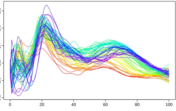
Age-sex specific data for Sweden are available for the years 1751–2007 fromHuman Mortality Database(2010). The data consist of central death rates and mid-year populations by sex and single years of age to 110 years. We group the data at ages 100 and above in order to avoid problems associated with erratic rates at these ages. We restrict the data to 1950–2007, but this has minimal effect because the weighted fitting procedure gives greater weight to recent data. Figures 1(a) and 1(b) show log death rates for males and females for selected age groups as univariate time series. Figure 2represents the same data as a series of smoothed curves
(functional observations). We use rainbow plots (Hyndman and Shang 2010) with the time
ordering of curves indicated by the colors of the rainbow, from red to violet. For females, mortality has declined steadily at most ages. For males, however, the decline stagnated at most adult ages in the 1960s and early 1970s. In recent years, male and female mortality at ages 20 and 30 are no longer declining, and small numbers of deaths result in relatively large fluctuations at age 10.
Figures3and4show the product function (on the log scale) and the ratio function of observed rates. The product function is the geometric mean of smoothed male and female rates; while in
1950 1970 1990 2010 −8 −6 −4 −2 Males Year Log death r ate 0 10 20 30 40 50 60 70 80 90 100 1950 1970 1990 2010 −8 −6 −4 −2 Females Year Log death r ate 0 10 20 30 40 50 60 70 80 90 100
Figure 1:Log death rates for males and females in Sweden for various ages as univariate time series.
0 20 40 60 80 100 −8 −6 −4 −2 Males Age Log death r ate 0 20 40 60 80 100 −8 −6 −4 −2 Females Age Log death r ate
Figure 2:Smoothed log death rates for males and females in Sweden viewed as functional time
series, observed from 1950 to 2007. Penalized regression splines with a partial monotonic
0 20 40 60 80 100 −8 −6 −4 −2 0 Age Log of geometr ic mean death r ate
Figure 3:Product function of the coherent functional model for Swedish data (1950–2007).
0 20 40 60 80 100 0.8 1.0 1.2 1.4 1.6 1.8 Age Se x r atio of death r ates: sqr t(M/F)
general this mean declines over time, recent increases are observed at ages 15 to 30, and at ages 1 to 5. The ratio function is the square root of the sex ratio of smoothed rates. Sex ratios of less than one occur where small numbers of deaths result in large random variation – at very young ages in recent years and at very old ages in earlier years. Since the 1980s, the ratio function has declined at ages 40 to 80, and more recently for older ages. In recent years, large fluctuations occur at ages less than 10 and at 20 to 30.
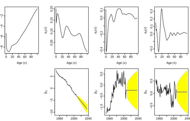
Figures 5 and 6 show the basis functions and corresponding coefficients with thirty year forecasts, produced by applying functional time series models to the product and ratio functions respectively. In the product model, the first principal component shows a declining trend in mortality, which is fastest at childhood ages and slowest at about age 20 and at very old ages. This term alone accounts for 97.0% of total variation. In the ratio model, the first principal component shows if anything a downward trend, but after 1990 fluctuations are substantial. This term accounts for 57.9% of total variation; the second and third terms account for 15.8% and 8.5% of total variation respectively. No cohort effects were observed in the residuals for the models.
Figure7shows thirty-year forecasts for male and female log death rates using the coherent functional model. The sex ratios of forecast death rates are shown in Figure 8, where they are also compared with sex ratios resulting from independent forecasts based on functional
time series models for separate male and female rates (following the approach ofHyndman
and Booth 2008). The coherent model produces sex ratios that are greater than one at all ages and remain within the limits of the observations on which they are based. In contrast, the independent models produce forecast sex ratios that are less than one at childhood ages and exceed the limits of observation at approximately ages 25 to 30 and 75+.
Thirty-year life expectancy at birth forecasts by sex are shown in Figure9, along with the sex difference in forecast life expectancy at selected ages. The forecasts based on independent models (dashed lines) are diverging, a feature that goes against recent trends, and leads to sex gaps in life expectancy at older ages that exceed observation. In contrast, the sex differences embodied in the forecasts based on the coherent method continue to decrease, and all tend towards approximately constant positive differentials. Thus, the coherent method produces sex differentials in both death rates and life expectancies that are in keeping with the levels and trends of the last 30 years.
0 20 40 60 80 −8 −6 −4 −2 Age (x) µ ( x ) 0 20 40 60 80 0.05 0.10 0.15 0.20 Age (x) φ1 ( x ) Time (t) βt1 1960 2000 2040 −10 −5 0 5 0 20 40 60 80 −0.4 −0.2 0.0 0.1 Age (x) φ2 ( x ) Time (t) βt2 1960 2000 2040 −1.0 −0.5 0.0 0.5 0 20 40 60 80 −0.2 0.0 0.1 0.2 0.3 Age (x) φ3 ( x ) Time (t) βt3 1960 2000 2040 −0.5 0.0 0.5
Figure 5:The first three basis functions and the corresponding coefficients of the product model for
Swedish data along with thirty-year forecasts and 80% prediction intervals using ARIMA models. 0 20 40 60 80 0.1 0.2 0.3 0.4 0.5 Age (x) µ ( x ) 0 20 40 60 80 −0.1 0.0 0.1 0.2 0.3 Age (x) φ1 ( x ) Time (t) βt1 1960 2000 2040 −0.8 −0.4 0.0 0.4 0 20 40 60 80 −0.2 0.0 0.1 0.2 Age (x) φ2 ( x ) Time (t) βt2 1960 2000 2040 −0.6 −0.2 0.2 0.4 0.6 0 20 40 60 80 −0.4 −0.2 0.0 0.1 0.2 Age (x) φ3 ( x ) Time (t) βt3 1960 2000 2040 −0.4 0.0 0.2 0.4 0.6
Figure 6:The first three basis functions and the corresponding coefficients of the ratio model for
Swedish data along with thirty-year forecasts and 80% prediction intervals using stationary ARFIMA models.
0 20 40 60 80 100 −10 −8 −6 −4 −2 Males Age Log death r ate 0 20 40 60 80 100 −10 −8 −6 −4 −2 Females Age Log death r ate
Figure 7:Thirty-year mortality forecasts for males and females in Sweden using the coherent
func-tional model.
The prediction intervals for life expectancies shown in Figure9are obtained from the percentiles of simulated life expectancy values, which in turn are obtained from simulated future mortality rates as described inHyndman and Booth(2008). A feature of this method is that it takes account of the nonlinear relationship between mortality rates and life expectancy, thus producing asymmetric intervals.
To examine forecast accuracy, Figure10shows out-of-sample MSFE values of log death rates based on equation (9). It is seen that both the coherent and independent models are more accurate for female than for male mortality, but that this sex difference is much smaller in the coherent case. The coherent model is more accurate than the independent model for male mortality, but less accurate for female mortality. The better performance for male mortality is attained at the expense of accuracy for female mortality, resulting in greater similarity in the degree of forecast accuracy for the two sexes. In overall terms, the coherent method performs marginally better (an average MSFE of 0.259 compared with 0.264 for the independent models). Thus, solving the problem of divergence has not resulted in a reduction in overall accuracy.
0 20 40 60 80 100 1.0 1.5 2.0 2.5 3.0 3.5 Coherent forecasts Age Se x r atio of r ates: M/F 0 20 40 60 80 100 1.0 1.5 2.0 2.5 3.0 3.5 Independent forecasts Age Se x r atio of r ates: M/F
Figure 8:Thirty-year forecasts of mortality sex ratios in Sweden using coherent and independent
functional models.
Life expectancy forecasts
Year Y ears 1960 1980 2000 2020 2040 70 75 80 85 1960 1980 2000 2020 2040 70 75 80 85
Life expectancy differences: F−M
Year Y ears 1960 1980 2000 2020 0 1 2 3 4 5 6 0 25 50 75 85 95
Figure 9:Thirty-year life expectancy forecasts for males and females in Sweden using coherent models
(solid lines) and independent models (dotted lines). Blue is used for males and red for females.
0 5 10 15 20 25 30 0.1 0.2 0.3 0.4 0.5 Forecast horizon MSFE Female Coherent Female Independent Male Coherent Male Independent
Figure 10:Forecast accuracy of coherent and independent models for different forecast horizons,
showing out-of-sample MSFE of log death rates.
3.2 Application to Australian state-specific mortality
In the second application, we consider the six states of Australia: Victoria (VIC), New South Wales (NSW), Queensland (QLD), South Australia (SA), Western Australia (WA) and Tasmania (TAS). The Australian Capital Territory and the Northern Territory are excluded from the analysis due to a large number of missing values in the available data. For each state, age-specific death rates and corresponding populations for 1950 to 2003 are obtained fromHyndman(2008). The ranking of life expectancy by state has changed over the fitting period; by 2003 the highest life expectancy occurred in Western Australia and Victoria and the lowest (by a margin of more than one year) in Tasmania.
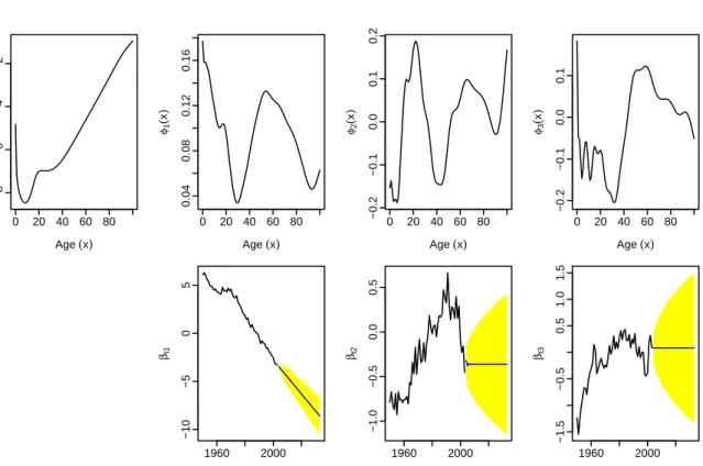
Figure11shows the first three basis functions of the product model and their coefficients along with thirty year forecasts. The first principal component of the product model accounts for 96.5% of total variation. The first three principal components of the ratio model for Victoria are plotted in Figure12. The first term accounts for 37.0% of total variation, the second accounts for 13.5% and the third for 9.2%. For other states, the first term accounted for between 28.7% and 52.1% of the total variation. (Ratio models for other states are not shown.) No cohort effects were observed in the residuals for the models.
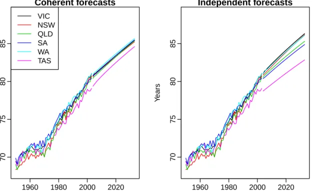
Figure13shows thirty-year life expectancy forecasts by state produced by the coherent and independent models. The life expectancy forecasts from the independent models are diverging,
0 20 40 60 80 −8 −6 −4 −2 Age (x) µ ( x ) 0 20 40 60 80 0.04 0.08 0.12 0.16 Age (x) φ1 ( x ) Time (t) βt1 1960 2000 −10 −5 0 5 0 20 40 60 80 −0.2 −0.1 0.0 0.1 0.2 Age (x) φ2 ( x ) Time (t) βt2 1960 2000 −1.0 −0.5 0.0 0.5 0 20 40 60 80 −0.2 −0.1 0.0 0.1 Age (x) φ3 ( x ) Time (t) βt3 1960 2000 −1.5 −0.5 0.5 1.0 1.5
Figure 11:The first three basis functions and their coefficients for the product model given in(5a)
for all states of Australia. Forecasts and 80% prediction intervals were obtained using ARIMA models. 0 20 40 60 80 −0.20 −0.10 0.00 Age (x) µ ( x ) 0 20 40 60 80 0.0 0.1 0.2 0.3 Age (x) φ1 ( x ) Time (t) βt1 1960 2000 −1.0 −0.5 0.0 0.5 0 20 40 60 80 −0.4 −0.2 0.0 0.1 0.2 Age (x) φ2 ( x ) Time (t) βt2 1960 2000 −0.4 −0.2 0.0 0.2 0.4 0 20 40 60 80 −0.1 0.0 0.1 0.2 0.3 Age (x) φ3 ( x ) Time (t) βt3 1960 2000 −0.4 0.0 0.2 0.4 0.6
Figure 12:The first three basis functions and their coefficients for the VIC ratio model given in(5b).
Coherent forecasts Year Y ears 1960 1980 2000 2020 70 75 80 85 VIC NSW QLD SA WA TAS Independent forecasts Year Y ears 1960 1980 2000 2020 70 75 80 85
Figure 13:Thirty-year life expectancy forecasts for Australian states using the coherent and
indepen-dent functional models.
whereas the forecasts from the coherent model are approximately converging towards a set of near-constant differences. For the coherent forecasts, the ranking of the six states changes over the forecast horizon, though Western Australia and Tasmania maintain their 2003 positions as highest and lowest respectively. The overall differential between the highest and lowest values and the differentials between states are consistent with observation.
Figure14shows out-of-sample MSFE values using coherent and independent models for the
Australian state data. The coherent model is more accurate at all horizons for four of the six state forecasts (the greatest loss of accuracy is for New South Wales). The increase in accuracy is greatest for Tasmania, which might be regarded as an outlier by 2003. On average, the coherent model performs slightly better (average MSFE of 0.325 compared with 0.346 for the independent models).
0 5 10 15 20 25 30 0.1 0.2 0.3 0.4 0.5 0.6 0.7 Forecast horizon MSFE VIC Coherent VIC Independent NSW Coherent NSW Independent QLD Coherent QLD Independent SA Coherent SA Independent WA Coherent WA Independent TAS Coherent TAS Independent
Figure 14:Forecast accuracy of coherent and independent models showing out-of-sample MSFE of log
death rates for Australian states.
4
Discussion
In this paper, we have proposed a new method for coherently forecasting the age-specific death rates of two or more subpopulations such that the resulting forecasts do not become divergent in the long term. The product-ratio functional method is based on functional forecasting of simple functions of the products and ratios of the subpopulation death rates, rather than the rates themselves. Using two-sex data for Sweden and six-state data for Australia, we have demonstrated the coherence of our results, while also demonstrating that the coherent method is at least as accurate in overall terms as independent forecasts.
4.1 Product-ratio method
The use of products and ratios is a simple and interpretable way of imposing coherence on the forecasts. The product function represents the geometric mean of subpopulation death rates — a version of the familiar mortality schedule. The ratio function is the ratio of the death rates of a particular subpopulation to the geometric mean rates; in the two-sex case, this is simply the square root of the sex ratio (and its inverse). Being a relative measure, the ratio function is easily understood and has the advantage of direct comparability over age (Figure4).
The use of the product and ratio functions also greatly simplifies the modelling procedure compared with the direct use of rates because the two functions are uncorrelated. The resulting model is elegant in its simplicity. The new method ensures coherence in terms of long-term non-divergence of forecast rates and produces results that remain within the observed range of variation for mortality ratios of subpopulations. Differentials between subpopulations tend to an approximate constant. The product-ratio method can handle outliers; in such cases the ratio function is larger than for other subpopulations and may have a different age pattern, but the forecast ratio function is kept within observed bounds.
An important advantage of the product-ratio method is greater flexibility in the age pattern of change in forecast mortality. When the product and ratio functions are combined to produce subpopulation mortality rates, the age pattern of mortality embodied in the product function is modified in accordance with the age pattern of the ratio function. Where the ratio function is close to 1, there is little modification of the geometric mean mortality rate; where the ratio function differs from 1, the geometric mean mortality rate is significantly modified (by multiplying by the ratio). The forecast product function is typically governed by an almost constant age pattern of change, because of a dominant first principal component. In contrast, several principal components are typically required to model the more complex ratio function, producing a variable age pattern of change over time. This variable pattern of change in the ratio function provides flexibility in the age pattern of change in mortality forecasts. The product-ratio functional approach thus allows for greater flexibility of change over time than the independent functional approach. Further, even if using only one principal component to model the product and the ratio functions — and hence fixed patterns of change for both — the product-ratio approach would allow flexibility of change in forecast mortality. The new approach allows for evolving ratios among forecast subpopulation rates (for example, sex ratios of forecast rates); this is in contrast to the Li and Lee approach where the ratios remain fixed over time (Li and Lee 2005, p582).
A limitation of the product-ratio method is that the long-term forecasts of the ratio function will converge to the mean ratios, which are determined by the choice of fitting period. We address this limitation in two ways. First the functional model that we employ incorporates weights that give greater weight to recent data (Hyndman and Shang 2009), so the long-term forecasts will converge to approximately the weighted mean ratios which are largely immune to the earliest data. (In our applications we use a weight parameter of 0.05 which has the
0.05(0.95)2= 0.0451 to the year before that, and so on.) Second, we use ARFIMA models for the coefficients of the ratio function; these models converge very slowly to the mean of the historical values of the coefficients. Tests were conducted to evaluate the possibility of basing the ratio function on a shorter fitting period, while maintaining the longer fitting period for the product function; this made almost no difference to average MSFE values, but destabilised the ratio forecast. The price of slow convergence using ARFIMA models is that a longer data series is needed for stable estimation. The full fitting period was therefore used for both functions. The use of the longer period for the ratio function may also be justified on conceptual grounds in that coherence implies that the sex ratios are stochastically stable over time.
4.2 Forecasts
The results for Sweden show a life expectancy at birth in 2037 of 86.4 years for females and 82.9 years for males. The forecast sex gap decreases from 4.0 years in 2007 to 3.5 years in 2037. Similarly for life expectancy at all other ages, the forecast sex gap decreases with slow convergence towards positive values.
The exact trajectory of this convergence and the long-term sex gap in life expectancy depend on the particular product and ratio functions. For life expectancies at younger ages, a fixed pattern of ratios produces a marginally smaller sex gap when product mortality is lower; thus some narrowing of the sex gap will occur independently of changing ratios. This effect may be reversed for life expectancies at older ages (70+ in the results for Sweden). Thus, while forecast death rates are constrained to tend towards a defined differential, forecast life expectancies are less precisely constrained.
The coherence embodied in the product-ratio method applies at all ages, as seen in the case of Sweden in the sex gaps in life expectancies at different ages (Figure9). Figure15shows results for four additional populations (the US, Canada, UK and France), illustrating a range of outcomes. In all cases, the sex gap in forecast life expectancies from the coherent model is well-behaved over both time and age.
The forecast life expectancies at birth in 2037 imply average annual increments of 0.113 years for females and 0.138 years for males. These are less than the average annual increments over the fitting period, implying deceleration in the rate of increase. For females, deceleration is in fact observed over the fitting period (9), and is continued in the forecast.Bengtsson(2006) notes that deceleration has been a recent feature of several formerly leading countries of female life
USA Year Y ears 1960 1980 2000 2020 0 2 4 6 8 0 25 50 75 85 95 Canada Year Y ears 1960 1980 2000 2020 0 2 4 6 8 0 25 50 75 85 95 UK Year Y ears 1960 1980 2000 2020 0 2 4 6 8 0 25 50 75 85 95 France Year Y ears 1960 1980 2000 2020 0 2 4 6 8 0 25 50 75 85 95
Figure 15:Differences in life expectancy forecasts for males and females (F–M) for 2008–2037 using
coherent models (solid lines) and independent models (dotted lines).
expectancy. For males, the linear trend since 1980 in observed life expectancy is not continued in the forecast.
While approximate linearity has been observed in the recent life expectancies of developed countries (White 2002), it is also the case that approximate linearity is observed in the coefficient of the first principal component of models of death rates (Lee 2006). When linearity is continued in the forecast of the coefficient, it does not produce linearity in forecast life expectancy. The main reason for this is that the principal component model assumes a fixed age pattern of change, whereas life expectancy takes into account the fact that the age pattern of change varies over time (Booth et al. 2002b). This is illustrated in Figure16for Swedish female mortality. The pessimistic forecast is based on a functional model using a single principal component with linear coefficient, and hence a fixed age pattern of change. The optimistic forecast is a random walk with drift model of life expectancy. This latter model is heavily dependent on the fitting
Forecasts of life expectancy at birth Year Y ears 1960 1980 2000 2020 2040 75 80 85
Figure 16:Forecasts of Swedish female life expectancy at birth from a random walk with drift model
applied directly to life expectancy data (red line) and a single principal component with
linear coefficient (blue line).
period, and in particular on the first year of the fitting period. If we were to discount the first few years of the fitting period, when the trend is particularly steep, a more gradual increase in forecast life expectancy would result, but this would still be greater than the increase embodied in the single principal component model.
In the Swedish example, several additional interconnected factors contribute to the relatively slow and diminishing increase in forecast life expectancy. Change in the product function, which is the main determinant of the trend in forecast male and female life expectancies, is more closely linear than in either male or female mortality (as determined by the independent models). This contributes to the result that linear change (the first principal component seen in Figure5) accounts for the very high percentage of variability after smoothing, which means that the functional forecast of the product term is effectively based on the single linear principal component, and the age pattern of change is fixed. Thus the forecast of product function mortality embodies a deceleration in the increase in life expectancy. In 2037, the forecast of geometric mean mortality is 86.4 years, equivalent to an average annual increase of 0.113 years. When there is almost total dominance of the first principal component in the product model, the forecast trend can be heavily dependent on the fitting period (especially if a random walk with
drift model is used, which depends totally on the first year and last year of the fitting period). In the Swedish example, the ARIMA(0,1,1) model (with drift) used for the first coefficient somewhat reduces this dependence by giving extra weight to more recent years. Further, we have used weighted functional methods to give greater weight to the more recent data and reduce dependence on the particular fitting period; however, this has little effect in the Swedish example because of linear change in the product function over the fitting period (Figure5). In other work, we have found the first principal component to account for about 94% of variation (Hyndman and Booth 2008), allowing some influence of the second and higher principal components in the forecast. The main effect of the additional principal components is to modify the age pattern of change embodied in the first principal component, so that the overall age pattern of change is not fixed. This has the effect of modifying the annual increments in forecast life expectancy.
For Sweden, the ratio model allows for greater flexibility over time in the age pattern of change. For example, one effect of the first principal component is the shifting of the primary mode of the ratio function to slightly older ages over the course of the fitting period, while the second component is largely responsible for the increase and then decrease in the secondary mode and also contributes to shifting it to older ages. At the oldest ages, there is little movement over time. In the forecast, the shifts are reversed because the pattern of change tends towards the weighted mean ratio function, but there is relatively little movement over the forecast horizon. At childhood ages, the forecast involves an increase in the ratio — in other words, female rates are declining faster than male, and the female advantage is increased. At young adult ages (roughly 20 to 30), this trend is reversed — the female advantage is reduced. Very little change is forecast at about ages 30 to 45. At about ages 45 to 70, the female advantage is increased, while at older ages it is slowly reduced over time in line with recent trends whereby male mortality disadvantage has diminished.
When the forecast ratio functions for male and female mortality are applied to the forecast product function, the resulting life expectancies are not equidistant from geometric mean life expectancy. Two factors contribute to this result. First, though symmetric on the log scale, the sex ratio and its inverse are asymmetric in their effects on product death rates: the larger effect occurs for males. Second, the effect of a constant ratio is greater for lower death rates. Both factors produce a greater difference from geometric mean life expectancy for male mortality than for female mortality. However, these differences are slight and the main determinant of the
trends in male and female forecast life expectancy is the forecast of geometric mean mortality. This explains why male forecast life expectancy decelerates more rapidly than does female life expectancy.
The forecast results for Australian states show slow convergence to approximately constant differences in life expectancy. The average forecast rate of increase is less than the observed average. As in the case of Sweden, the dominant first principal component of the product function (a linear coefficient with fixed age pattern of change) produces slightly convex forecasts of life expectancy.
4.3 Forecast accuracy
It has been shown that the product-ratio functional method ensures non-divergence without compromising the overall (average) accuracy of the forecasts. In the two-sex case, the accuracy of the male mortality forecast was improved at the expense of accuracy in female mortality forecast; in other words, by adopting the coherent method, the accuracy of the forecasts for the two sexes was (partly) equalised. Similarly in the six-state example, forecast accuracy is more homogeneous in the coherent method, with an improvement in overall accuracy. This feature of the method is useful in practical applications such as population forecasting, where it is preferable to maintain a balanced margin of error and hence a more balanced forecast population structure than might occur in the independent case. Similarly in financial planning, it may be preferable to accept moderate error in all subpopulations rather than risk a large error in one subpopulation.
Coherent forecasting incorporates additional information into the forecast for a single sub-population. The additional information acts as a frame of reference — limiting the extent to which a subpopulation forecast may continue a trend that differs from that of trends in related subpopulations. A similar approach has previously been adopted byOrtega and Poncela(2005) in forecasting fertility, as well as byLi and Lee(2005) for mortality.
The use of additional information raises the question of the choice of information. How impor-tant is it that the subpopulations be appropriately chosen? In the two-sex case, where data for both females and males are used to forecast mortality for each sex, the choice is pre-determined. Similarly, there is little doubt about the appropriateness of geographic subpopulations of a country. The grouping of several countries, however, is less clear (Li and Lee 2005). We note that the ‘outlier’ state of Tasmania has been successfully forecast, and similar results can be
expected for countries that might be considered outliers in a larger region. The product-ratio method is relatively insensitive to the composition of the product function because of the simpler orthogonal relationship between the product and ratio functions (compared with the more complex correlated relationship between the group and individual rates used by Li and Lee).
Evidence suggests that the product-ratio functional method may produce more accurate forecasts than other methods. The evaluations ofBooth et al.(2006) show that the functional data model ofHyndman and Ullah(2007) produces more accurate forecasts of death rates than the Lee-Carter method and its variants in 13 out of 20 populations. In this research we have used an
improved functional data model which incorporates weights (Hyndman and Shang 2009), and
has been shown to produce more accurate forecasts than any other method based on a principal components decomposition including the Lee-Carter variant used by Li and Lee (Shang et al. 2010). To compare our results for Sweden with those ofLi and Lee(2005) we extended our forecasts to 2100: the product-ratio method produced a sex gap in life expectancy at birth of 2.2 years compared with 3.0 years by the Li-Lee method. Forecast life expectancy in 2100 was 91.3 years for females and 89.1 years for males, compared with approximately 93 and 90 years respectively fromLi and Lee(2005). Further research is needed to fully evaluate methods for coherent mortality forecasting.
4.4 Generalisation of the Li-Lee method
The product-ratio functional method can be viewed as a generalisation of theLi and Lee(2005) approach.Li and Lee(2005) employed the following model, expressed here for the two-sex case using notation consistent with that used in Section2:
yt,j(x) =µj(x) +βtφ(x) +γt,jφj(x) +et,j(x) (10)
wherej∈ {F, M},βt is a random walk with drift,φ(x) is the first principal component of the
common factor Lee-Carter model (based on combined male and female data),γt,j is an AR(1) process, φj(x) is the first principal component of the residual matrix of the common factor
model, andet,j(x) is the error. The residual matrix is based onβt after adjustment to match annual life expectancy (Lee and Miller 2001b). Coherency is achieved by modellingγt,j as an
There are several points of difference betweenLi and Lee(2005) and the product-ratio functional method. First,Li and Lee(2005) use a single principal component in each model, while we use up to six (Hyndman and Ullah 2007) — though in practice only the first two have much effect for mortality. The additional principal components capture patterns in the data thatwhich are supplementary to the main trend and which may be significant. Booth et al.(2006, Table 3) showed that methods involving additional principal components were at least as accurate in 16 of 20 populations. The incorporation of additional principal components has the advantage that modelled death rates are no longer perfectly correlated across age (which is a feature of single component models). The use of the multiple principal components does not add significantly to the complexity of the model because the γt,`,` = 1, . . . , L coefficients are uncorrelated by
construction; there is thus no need to employ a vector approach.
Second,Li and Lee(2005) restrict the time series models to a random walk with drift forβt
and an AR(1) process forγt,j, whereas we allow more varied dynamics to be modelled through
more general ARIMA processes for each βt,`, ` = 1, . . . , L and any stationary ARMA(p, q) or
ARFIMA(p, d, q) process for eachγt,`,`= 1, . . . , L. Third, in theLi and Lee(2005) approach, the
γt,j coefficients are highly correlated with each other (over), necessitating a vector approach
Reinsel(2003) for modelling theγt,j coefficients, which adds considerably to the complexity of
the method.
Finally, by modellingyt,j instead offt,j, theLi and Lee(2005) model includes observational
error which will be propagated in the forecasts. In the functional approach, observational error is removed by smoothing and added back in after modelling as part of variance estimation. Thus theLi and Lee(2005) model can be considered a special case of the more general product-ratio functional method — the case where there is no smoothing, each model has only one component, and the time series models used are either a random walk with drift or a first order autoregression.
4.5 Extensions and practical application
A possible extension of the method would be to incorporate two or more dimensions in defining the product, so as to obtain coherency between and within each dimension; for example, sex and state might be used to coherently forecast male and female mortality within state, and mortality by state within each sex. A further possible but less elegant extension is the use of an external standard mortality schedule in place of the product, combined with ratios of subpopulations to
this standard. This option may be useful where data for the appropriate group are missing. Best practice mortality (Oeppen and Vaupel 2002) may provide a useful standard. Further research is needed to examine these possibilities in greater detail.
Finally, it should be acknowledged that the development of improved forecasting methods for mortality, and by extension for fertility and migration (Hyndman and Booth 2008), represents a step towards more reliable and more easily automated demographic forecasting and the acceptance of these stochastic methods by national statistical offices responsible for producing official population projections. Though more complex than traditional methods, these methods
are easily accessible through user-friendly code now available on CRAN (Hyndman 2010).
Application of the methods is considerably simplified by this free software.
References
Bengtsson, T. (2006), Linear increase in life expectancy: past and present, in T. Bengtsson, ed., ‘Perspectives on Mortality Forecasting III. The Linear Rise in Life Expectancy: History and Prospects’, Social Insurance Studies No.3, Swedish Social Insurance Agency, Stockholm, pp. 83–99.
Booth, H., Hyndman, R. J., Tickle, L. & de Jong, P. (2006), ‘Lee-Carter mortality forecasting: a multi-country comparison of variants and extensions’,Demographic Research15(9), 289–310. Booth, H., Maindonald, J. & Smith, L. (2002a), ‘Applying Lee-Carter under conditions of variable
mortality decline’,Population Studies56(3), 325–336.
Booth, H., Maindonald, J. & Smith, L. (2002b), ‘Applying Lee-Carter under conditions of variable mortality decline’,Population Studies56(3), 325–336.
Booth, H. & Tickle, L. (2008), ‘Mortality modelling and forecasting: A review of methods’,
Annals of Actuarial Science3(1-2), 3–43.
Box, G. E. P., Jenkins, G. M. & Reinsel, G. C. (2008),Time series analysis: forecasting and control, 4th edn, John Wiley & Sons, Hoboken, NJ.
Cairns, A., Blake, D. & Dowd, K. (2006), ‘A two-factor model for stochastic mortality with parameter uncertainty: Theory and calibration’,Journal of Risk and Insurance73, 687–718.
Cairns, A., Blake, D., Dowd, K., Coughlan, G. & Khalaf-Allah, M. (2008), ‘Mortality density forecasts: An analysis of six stochastic mortality models’,Pensions Institute Discussion Paper
PI-0801.64.
Currie, I. D., Durban, M. & Eilers, P. H. (2004), ‘Smoothing and forecasting mortality rates’,
Statistical Modelling4, 279–298.
Granger, C. & Joyeux, R. (1980), ‘An introduction to long-memory time series models and fractional differencing’,Journal of Time Series Analysis1, 15–39.
Haslett, J. & Raftery, A. E. (1989), ‘Space-time modelling with long-memory dependence: Assessing Ireland’s wind power resource (with discussion)’,Applied Statistics38, 1–50. Hosking, J. (1981), ‘Fractional differencing’,Biometrika68, 165–176.
Human Mortality Database (2010), University of California, Berkeley (USA), and Max Planck Institute for Demographic Research (Germany). Downloaded on 14 October 2010.
URL:www.mortality.org
Hyndman, R. J. (2008),addb: Australian Demographic Data Bank. R package version 3.222.
URL:robjhyndman.com/software/addb
Hyndman, R. J. (2010),demography: Forecasting mortality, fertility, migration and population data. R package version 1.07.
URL:robjhyndman.com/software/demography
Hyndman, R. J. & Booth, H. (2008), ‘Stochastic population forecasts using functional data models for mortality, fertility and migration’,International Journal of Forecasting24(3), 323–342. Hyndman, R. J. & Khandakar, Y. (2008), ‘Automatic time series forecasting: The forecast package
for R’,Journal of Statistical Software26(3).
Hyndman, R. J. & Shang, H. L. (2009), ‘Forecasting functional time series (with discussion)’,
Journal of the Korean Statistical Society38(3), 199–221.
Hyndman, R. J. & Shang, H. L. (2010), ‘Rainbow plots, bagplots and boxplots for functional data’,Journal of Computational & Graphical Statistics19(1), 29–45.
Hyndman, R. J. & Ullah, M. S. (2007), ‘Robust forecasting of mortality and fertility rates: a functional data approach’,Computational Statistics & Data Analysis51, 4942–4956.
Lee, R. D. (2000), ‘The Lee-Carter method for forecasting mortality, with various extensions and applications’,North American Actuarial Journal4(1), 80–92.
Lee, R. D. (2006), Mortality forecasts and linear life expectancy trends, inT. Bengtsson, ed., ‘Perspectives on Mortality Forecasting: Vol. III. The Linear Rise in Life Expectancy: History and Prospects’, Social Insurance Studies No.3, Swedish National Social Insurance Board, Stockholm, pp. 19–39.
Lee, R. D. & Carter, L. R. (1992), ‘Modeling and forecasting US mortality’,Journal of the American
Statistical Association87(419), 659–671.
Lee, R. D. & Miller, T. (2001a), ‘Evaluating the performance of the Lee-Carter method for forecasting mortality’,Demography38(4), 537–549.
Lee, R. D. & Miller, T. (2001b), ‘Evaluating the performance of the Lee-Carter method for forecasting mortality’,Demography38(4), 537–549.
Lee, R. & Nault, F. (1993), ‘Modeling and forecasting provincial mortality in Canada’. Paper presented at the World Congress of the IUSSP, Montreal, Canada.
Li, N. & Lee, R. (2005), ‘Coherent mortality forecasts for a group of populations: An extension of the Lee-Carter method’,Demography42(3), 575– 594.
Oeppen, J. (2008), Coherent forecasting of multiple-decrement life tables: a test using Japanese cause of death data, Technical report, Universitat de Girona. Departament d’Inform`atica i Matem`atica Aplicada.
URL:http://hdl.handle.net/10256/742
Oeppen, J. & Vaupel, J. W. (2002), ‘Broken limits to life expectancy’,Science296(5570), 1029– 1031.
URL:http://www.sciencemag.org/cgi/reprint/296/5570/1029.pdf
Ortega, J. A. & Poncela, P. (2005), ‘Joint forecasts of southern European fertility rates with non-stationary dynamic factor models’,International Journal of Forecasting21(3), 539–550. Peiris, M. & Perera, B. (1988), ‘On prediction with fractionally differenced ARIMA models’,
Journal of Time Series Analysis9(3), 215–220.
popula-Reinsel, G. C. (2003),Elements of Multivariate Time Series Analysis, second edn, Springer. Renshaw, A. & Haberman, S. (2003), ‘Lee–Carter mortality forecasting: A parallel
general-ized linear modelling approach for England and Wales mortality projections’,Appl. Statist. 52(1), 119–137.
Shang, H. L., Booth, H. & Hyndman, R. J. (2010), A comparison of ten principal component methods for forecasting mortality rates, Working paper 08/10, Department of Econometrics & Business Statistics, Monash University.
Shumway, R. H. & Stoffer, D. S. (2006),Time Series Analysis and Its Applications: With R Examples, 2nd edn, Springer, New York.
Tukey, J. W. (1977),Exploratory Data Analysis, Addison-Wesley, London.
URL:http://www.amazon.com/Exploratory-Data-Analysis-Wilder-Tukey/dp/B0007347RW
White, K. M. (2002), ‘Longevity advances in high-income countries, 1955-96’,Population and
Development Review28, 59–76.
Wilmoth, J. R. (1995), ‘Are mortality projections always more pessimistic when disaggregated by cause of death?’,Mathematical Population Studies5(4), 293–319.
Wood, S. N. (1994), ‘Monotonic smoothing splines fitted by cross validation’,SIAM J. Sci Comput 15(5), 1126–1133.