Essex Finance Centre
Working Paper Series
Working Paper No21: 09-2017
“Level Shift Estimation in the Presence of Non-stationary Volatility
with an Application to the Unit Root Testing Problem”
“David Harris, Hsein Kew and A.M. Robert Taylor”
Essex Business School, University of Essex, Wivenhoe Park, Colchester, CO4 3SQ Web site: http://www.essex.ac.uk/ebs/
Level Shift Estimation in the Presence of Non-stationary Volatility
with an Application to the Unit Root Testing Problem
∗David Harrisa, Hsein Kewb and A.M. Robert Taylorc
a Department of Economics, University of Melbourne
b Department of Econometrics and Business Statistics, Monash University c Essex Business School, University of Essex
Abstract
In this paper we contribute to two separate literatures. Our principal contribution is made to the literature on break fraction estimation. Here we investigate the properties of a class of weighted residual sum of squares estimators for the location of a level break in time series whose shocks display non-stationary volatility (permanent changes in unconditional volatility). This class contains the ordinary least squares (OLS) and weighted least squares (WLS) estimators, the latter based on the true volatility process. For fixed magnitude breaks we show that the estimator attains the same consistency rate under non-stationary volatility as under homoskedasticity. We also provide local limiting distribution theory for the estimator when the break magnitude is either local-to-zero at some rate in the sample size or exactly zero. The former includes the Pitman drift rate which is shown via Monte Carlo experiments to predict well the key features of the finite sample behaviour of the OLS estimator and a feasible version of the WLS estimator based on an adaptive estimate of the volatility path of the shocks. The simulations highlight the importance of the break location, break magnitude, and the form of non-stationary volatility for the finite sample performance of these estimators, and show that the feasible WLS estimator can deliver significant improvements over the OLS estimator in certain heteroskedastic environments. We also contribute to the unit root testing literature. We demonstrate how the results in the first part of the paper can be applied, by using level break fraction estimators on the first differences of the data, when testing for a unit root in the presence of trend breaks and/or non-stationary volatility. In practice it will be unknown whether a trend break is present and so we also discuss methods to select between the break and no break cases, considering both standard information criteria and feasible weighted information criteria based on our adaptive volatility estimator. Simulation evidence suggests that the use of these feasible weighted estimators and information criteria can deliver unit root tests with significantly improved finite sample behaviour under heteroskedasticity relative to their unweighted counterparts.
Keywords: Level break fraction, non-stationary volatility, adaptive estimation, feasible weighted estimator, information criteria, unit root tests and trend breaks.
JEL: C12, C22.
∗
We thank Giuseppe Cavaliere and participants at the International Conference in Celebration of the 65th Birthday of Maxwell King for useful comments. Taylor gratefully acknowledges financial support provided by the Economic and Social Research Council of the United Kingdom under research grant ES/M01147X/1. Correspondence to: Robert Taylor, University of Essex, Wivenhoe Park, Colchester, CO4 3SQ, United Kingdom. Email:[email protected].
1
Introduction
Breaks in the deterministic trend function appear prevalent in macroeconomic series; see,inter alia, Stock and Watson (1996,1999,2005) and Perron and Zhu (2005). The impact of these on standard unit root tests has been well known since the seminal work of Perron (1989). In his original work, Perron (1989) treated the location of potential breaks as known. Subsequent approaches have focused on the case where the break date is unknown and is replaced by a break fraction estimator; see,inter alia, Perron (1997) and Perron and Rodr´ıguez (2003). More recently, Harriset al. (2009) and Carrion-i-Silvestre et al. (2009), among others, extend these approaches to allow for the case where there is uncertainty as to whether a trend break has occurred by incorporating pre-test procedures for the presence of a trend break. Central to these approaches is an estimate of the break fraction and, in the case of the latter two, some form of pre-test for the presence of a break. Under a fixed magnitude trend break the break fraction estimator needs to be consistent at a rate
faster thanT−1/2,T denoting the sample size, for the resulting unit root test to be asymptotically valid in the case where a trend break occurs. As a result, the ordinary least squares [OLS] level break estimator of Bai (1994) has tended to be applied to the first differences of the series because it is consistent at rate T−1 for the true break fraction where a break occurs, while the corresponding OLS-based estimator of the trend break fraction in the levels is only consistent at rate T−1/2.
The aforementioned procedures, while allowing for the possibility of breaks in the deterministic trend function, do not allow for time-varying behaviour in the unconditional volatility (often re-ferred to as non-stationary volatility in the literature) of the driving shocks. This is an important practical drawback given that a large number of empirical studies have reported a substantial de-cline, often referred to as the Great Moderation, in the unconditional volatility of the shocks driving macroeconomic series in the twenty years or so leading up to the Great Recession that started in late 2007, with a subsequent sharp increase again in volatility observed after 2007; see, inter alia, McConnell and Perez-Quiros (2000), Clark (2009), Stock and Watson (2012), and the references therein. Cavaliere et al. (2011) refine the approach of Harriset al. (2009) to use wild bootstrap unit root tests. However, their procedures are still based around the applying the OLS level break fraction estimator of Bai (1994) to the first differences and trend break pre-test, each of which were developed for homoskedastic innovations. While they show that both of these (and, indeed, the resulting unit root procedures) are asymptotically robust to time-varying volatility, their finite sample efficacy will clearly have important forward implications for the behaviour of the resulting unit root tests.
Our principal aim in this paper is to explore the properties of the OLS level break estimator of Bai (1994), which is central to the unit root testing procedures discussed above, in cases where the shocks can display non-stationary volatility and to develop and explore the properties of a corre-sponding feasible weighted least squares [WLS] level break estimator based around the use of data which have been weighted by a non-parametric estimate of the volatility path. We will consider a set-up for the volatility process of a very general form, taken to be unknown to the practitioner, which allows, for example, single and multiple abrupt variance breaks, smooth transition variance breaks, and trending variances. We will also allow for the presence of conditional
heteroskedas-ticity in the shocks. The feasible WLS estimator we propose uses adaptive methods to estimate the volatility path of the shocks. Adaptive methods have been successfully employed in a number of areas of the literature including inference on the parameters of finite-order unconditionally het-eroskedastic autoregressive models by Phillips and Xu (2006) and Xu and Phillips (2008), testing for ARCH effects in unconditionally heteroskedastic autoregressive models by Patilea and Ra¨ıssi (2014), testing for long memory in unconditionally heteroskedastic ARFIMA models by Harris and Kew (2017) and adaptive testing for autocorrelation in Harris and Kew (2014), and for adaptive estimation of VAR models in Patilea and Ra¨ıssi (2012, 2013). Of most relevance to this paper, Boswijk and Zu (2017) propose an adaptive estimator of the unconditional variance process in the context of testing for a unit root in an autoregressive model driven by heteroskedastic errors, but where no allowance is made for the possibility of a trend break.
We establish the large sample properties of the OLS and feasible WLS break fraction estimators under a variety of assumptions on the magnitude of the level shift. For level shifts of either fixed (non-zero) magnitude or where the level shift magnitude is local-to-zero at a rate slower than the Pitman rate of T−1/2, we demonstrate the consistency of these estimators, and indeed those from a generic class of residual sums of squares [RSS] based break fraction estimators. This rate of consistency is shown to be the same for the OLS and feasible WLS estimators and to be unaffected by the location of the break or by time variation in the volatility process. We also derive the asymptotic distributions of these estimators in the case where the magnitude of the level shift lies within a Pitman neighbourhood of zero. Elliott and M¨uller (2007) argue that the finite sample behaviour of break fraction estimators such as those considered in this paper is likely to be far better approximated for the sort of break magnitudes typically encountered in practice by asymptotic theory based on a Pitman localisation rather than a fixed magnitude break. The results we present in this paper entirely accord with this viewpoint. Under Pitman drift the limiting distributions of the OLS and feasible WLS estimators are shown to differ and to depend on the location and (local drift) magnitude of the level break and, to differing extents, on the time variation in the volatility process. Monte Carlo simulations are used to investigate and compare the finite sample behaviour of the estimators and these are shown to agree closely with the qualitative predictions that we draw from the limiting distributions under Pitman drift. In particular, they highlight the importance of the break location, break magnitude, and the time path of the volatility process for the finite sample performance of these estimators. They also show that the feasible WLS estimator can deliver significant improvements over the OLS estimator in certain heteroskedastic environments, most notably in cases where the level break occurs in a low volatility regime.
We then investigate to what extent the improved behaviour we observe for the feasible WLS level break fraction estimator relative to the standard OLS estimator of Bai (1994) when non-stationary volatility is present can effect improvements in the finite sample behaviour of the unit root tests discussed above designed for the case where a trend break (might) occur in the data and where the shocks are heteroskedastic. Here we also propose model selection methods based on the familiar Schwarz (1978) criterion to select between the trend break and no trend break models in the practically relevant case where it is unknown whether a trend break is present in the data or not. We discuss such information criteria based on standard OLS model estimation
and on feasible WLS model estimation, the latter based on the same adaptive estimator of the unconditional variance process as used in constructing the feasible WLS break fraction estimator. Simulation evidence suggests that the use of these feasible weighted estimators and feasible weighted information criteria can deliver unit root tests with significantly improved finite sample behaviour in the presence of non-stationary volatility relative to using their unweighted counterparts.
The paper is organised as follows. Our reference heteroskedastic level break model is outlined in section 2. Section 3 outlines a generic RSS level break fraction estimator which contains the standard OLS estimator of Bai (1994) and the infeasible WLS estimator as special cases. Here we also show how a feasible version of the WLS estimator can be constructed, using an adaptive estimator of the volatility path of the innovations. The large sample properties of these estimators are compared for both fixed, local and zero magnitude level shifts. The relative finite sample properties of these estimators in both homoskedastic and a variety of heteroskedastic environments are explored in section 4. In section 5 the application of level break estimation methods to the problem of unit root testing when breaks in trend and/or volatility may be present is discussed. Section 6 concludes. All proofs are collected in a mathematical appendix. Further simulation results are included in a supplementary appendix.
In what follows, ‘b·c’ denotes the integer part, ‘1(.)’ denotes the indicator function, and ‘x:=y’ (‘x =: y’) indicates that x is defined by y (y is defined by x). The symbols ‘→d’ and ‘→p ’ are respectively used to denote convergence in distribution and probability respectively, as T → ∞. The maximum and minimum ofaandbare denoteda∨banda∧b, respectively. Finally,D:=D[0,1] denotes the space of right continuous with left limit (c`adl`ag) processes on [0,1].
2
The Heteroskedastic Level Break Model
We consider the time series process {yt} generated according to the following level break model,
yt = µ+δT ·1t>bτ0Tc+et (2.1)
et = σtεt. (2.2)
Equation (2.1) is seen to comprise the sum of a constant and level shift at time bτ0Tc, together with a stochastic component et, which we detail further below. As is standard, for the purposes of the large sample results which follow, we assume that the break date depends on the sample size such that the break occurs at a fixed fraction of the sample size; that is, we parameterise the breakpoint in terms of the break fraction τ0 where 0< τL≤τ0 ≤τU <1.
In order to allow for level breaks which are either of fixed magnitude or are local-to-zero at some rate in the sample size, T, we follow Elliott and M¨uller (2007) and parameterise the break magnitude parameter as δT := δT−d withδ a fixed constant and d≥0. It can be seen that for a given fixed value of T a level break exists inyt of (2.1) only ifδ6= 0. No break occurs when δ= 0, regardless of the value ofd, while a level break of fixed magnitudeδoccurs whend= 0 andδ 6= 0. In the unconditionally homoskedastic case, whereσt=σ for allt, Bai (1997), shows that whenδ6= 0, then τ0 is consistently estimated by least squares for any 0 ≤ d <1/2.1 In particular, although
1The consistency results given in Bai (1997) also hold in the case whereσ
the magnitude of the level break shrinks here as the sample size increases, the level break is still sufficiently large for the location of the break, τ0, to be consistently estimated and for consistent tests to exist for testing for a level break. Again in the unconditionally homoskedastic case, setting
d= 1/2 gives the Pitman drift rate for this problem such thatτ0 cannot be consistently estimated nor can a consistent test for the presence of a level break be obtained. We will show that these consistency rates in dalso hold in the heteroskedastic case we focus on in this paper.
To complete the specification of (2.1)-(2.2) the following conditions, collectively labelled As-sumption A, will be assumed to hold.
Assumption A.
A1. The innovations {εt} form a martingale difference sequence with respect to the filtration
Ft,where Ft−1 ⊆ Ft for t=...,−1,0,1,2, ...,satisfying: (i) the global homoskedasticity condition: 1
T
PT
t=1E ε2t|Ft−1 p
→1, and (ii)E|εt|r< K <∞for some r≥4;
A2. The volatility term σt satisfies σt = σ(t/T), where σ(·) ∈ D is non-stochastic, bounded
above and below as 0< σ≤σ(s)≤σ <¯ ∞ for all s,and satisfies a Lipschitz condition.
Remark 2.1. The process {et} in (2.2) is formed as the product of two components, {εt} and
{σt}. The former is assumed to satisfy a relatively weak globally stationary martingale difference assumption which allows for certain forms of conditional heteroskedasticity, such as that arising from stationary GARCH models, in the errors; see Davidson (1994, pp.454-455) for further discussion. Notice that, conditionally on σt, the error termethas mean zero and time-varying variance σt2.
Remark 2.2. Assumption A2 casts the dynamics of the disturbance variance in a quite general framework, requiring it only to be non-stochastic, bounded and to be smooth in between a countable number of jumps. A detailed discussion of the class of variance processes allowed underA2is given in Cavaliere and Taylor (2007). They show that this includes variance processes displaying multiple volatility shifts, polynomially (possibly piecewise) trending volatility and smooth transition variance breaks, among other things. In the case where volatility displays jumps, these are not constrained to be located at the same point in the sample as the putative level shift, nor indeed are they required to lie within the search set, Λ. The conventional unconditionally homoskedastic assumption that
σt=σ for all t, also satisfies Assumption A2, since here σ(s) =σ for all s.
Remark 2.3. In order to focus our attention on the impact of non-stationary volatility of the form considered in Assumption A2 on level break estimation, we have omitted autocorrelation in the model for the disturbanceet. We will, however, discuss generalisations to allow for this at relevant
points in the text.
3
Level Break Fraction Estimation
In this section we will consider level break fraction estimation based on the minimisation of a RSS criterion from a weighted regression model. In this general framework setting the weights to unity yields the OLS break fraction estimator while setting the weighting factor at time tto be equal to
the inverse of the volatility process at timetyields the corresponding weighted least squares [WLS] estimator. A generic form for this estimator is first given in section 3.1. In section 3.2, under the assumption of non-stochastic weights, we establish the large sample properties of this estimator under “large” magnitude breaks (where the magnitude is either fixed and non-zero or local-to-zero at a slower rate than the Pitman drift), demonstrating the consistency of the estimator in such cases. In section 3.3 we analyse, again for non-stochastic weights, the large sample behaviour of the estimator under “small” magnitude breaks (where the break magnitude is either exactly zero or local-to-zero at the Pitman rate or faster). In practice the volatility process is unknown and so a feasible version of the WLS estimator will require an estimate of the volatility process. In section 3.4 we show how this can be done using an adaptive estimator and demonstrate that the resulting feasible WLS break fraction estimator is asymptotically equivalent to the infeasible WLS estimator based on the true volatility process.
3.1 Residual Sum of Squares Break Fraction Estimator
In what follows we define a generic RSS-based level break fraction estimator which contains weighted and unweighted break fraction estimators as special cases. To that end, define the weights xt,
t= 1, ..., T, and a generic RSS-based estimator
ˆ τ := arg min τ∈[τL,τU] T X t=1 ˆ e∗τ,t2 (3.1)
where, for any τ ∈[τL, τU]⊂[0,1], the residuals ˆe∗τ,t are obtained from the OLS regression
y∗t = ˆµτxt+ ˆδτ(1t>bτ Tc·xt) + ˆe∗τ,t (3.2)
where y∗t := xtyt.2 Setting xt := 1 for t = 1, ..., T, in (3.2) yields the usual OLS estimator of τ0 considered in Bai (1994), while setting xt:= 1/σt,t= 1, ..., T, yields the infeasible WLS estimator that obtains with knowledge of σt. In what follows, where we wish to make reference to the OLS and WLS estimators specifically, rather than the generic RSS-based estimator in (3.1), we will use the notation ˆτOLS and ˆτW LS, respectively. The assumption of non-stochastic weights will be relaxed in section 3.4 when we detail our feasible WLS estimator of τ0 based on adaptive estimation ofσt.
3.2 Asymptotic Behaviour of τˆ under Large Breaks
We first analyse the large sample behaviour of ˆτ in the case where the trend break magnitude is “large” in that it can be either non-zero and fixed or is such that it is local-to-zero but at a rate slower than the Pitman drift rate of T−1/2. We will show that the standard OLS estimator of τ0 retains the consistency property established under unconditional homoskedasticity in Bai (1997) and that the rate also holds for the corresponding WLS estimator, and indeed for any of a wide class of weights. These results are now formally stated in Theorem 1.
2
The form of estimated coefficients ˆµτ and ˆδτ obviously depend on the choice ofxt but this is omitted from the
Theorem 1. Let yt be generated according to (2.1) with δT := δT−d and let Assumption A hold.
Moreover let the non-stochastic weights, xt =x(t/T), t = 1, ..., T, used in constructing τˆ of (3.1)
be such that x(.) satisfies the same conditions as σ(.) given in Assumption A2. Then ifδ 6= 0 and 0≤d <1/2, it holds that τˆ→p τ0. Moreover, if δ6= 0 and 0< d <1/2 then
T δT2x(τ0) 4 σ(τ0)2 (ˆτ −τ0) d →arg max s∈(−∞,∞)Z(s), (3.3) where Z(s) := W1(−s)−|2s|, s≤0 √ φW2(s)−ξ |s| 2, s >0
in which W1 and W2 are independent standard Brownian motions each on [0,∞), and
φ:= σ¯(τ0) 2x¯(τ 0)2 σ(τ0)2x(τ0)2 , ξ:= ¯ x(τ0) x(τ0) 2 ,
where σ¯(τ0) := limτ↓τ0σ(τ), σ(τ0) := limτ↑τ0σ(τ), x¯(τ0) := limτ↓τ0x(τ) and x(τ0) := limτ↑τ0x(τ).
Remark 3.1. From Theorem 1 we obtain that ˆτ is a consistent estimator for ˆτ at rateOp(T−1δT−2) and, hence, is a consistent estimator regardless of the value of d, provided 0< d <1/2, and irre-spective of any conditional or unconditional heteroskedasticity present inσt satisfying Assumption
A, or the form of the weights, xt, used in its construction. For the fixed break magnitude case whered= 0 andδ6= 0, (ˆτ−τ0) is of Op(T−1) under the conditions of AssumptionA; see Cavaliere
et al. (2011).
Remark 3.2. The results in Theorem 1 extend the results of Bai (1994) for the unweighted OLS estimator to cover both weighted and unweighted level break estimators and to allow for the general form of unconditional heteroskedasticity permitted in σtunder AssumptionA2. Bai (1997) establishes the same Op(T−1δT−2) rate in regression models (including (3.2)) allowing for weak dependence and conditional heteroskedasticity in the shocks, the latter of a similar form to that allowed under Assumption A1. We specify martingale difference disturbances here in to order to focus attention on the role of non-stationary volatility in this model, but it can also be shown that the Op(T−1δT−2) consistency rate given in Theorem 1 continues to hold whenet is autocorrelated. For example, ifet=σtutwhere, as in equation (2) of Bai (1994),utis generated by a linear process
ut=C(L)εt, where C(L) :=
P∞
j=0cjLj satisfies the standard summability condition (assumption B of Bai, 1994) P∞
j=0j|cj|<∞, and εt and σt again satisfy the conditions in AssumptionA, then the short run variance, σ(τ0)2, in (3.3) would simply need to be replaced by the corresponding long run variance, σ(τ0)2C(1)2.
Remark 3.3. A comparison of the results in Theorem 1 with the corresponding results in Propo-sition 3 of Bai (1997) shows that the presence of non-stationary volatility in et has no effect on the large sample properties of ˆτ, with the exception of the situation where a jump in the variance occurs at τ0 (a possibility also allowed for in the set-up considered by Bai, 1997) inducing the presence of the termsφand ξ inZ(s). Other than this,σt does not affect the limiting distribution of ˆτ. The weighting factor xt is also seen to make no difference to the asymptotic distribution of
ˆ
τ (again with the one exception where a breakx(s) occurs at τ0). Indeed, it can be seen that it is only the variance of the shocks at τ0 (or on either side of τ0 if the variance also changes at τ0) that features in this limit; that is, the prediction from the large sample result in Theorem 1 is that where a level break occurs, the efficacy of ˆτ is a function of the level break magnitude relative to the volatility of the shocks at that point in the sample only. As we will see in section 3.3, this contrasts with the “small” breaks asymptotics which predicts that the efficacy of ˆτ is a function of the level break magnitude relative to (a function of) the entire sample path of the volatility function, and, moreover, depends on the weighting factor used in constructing ˆτ. The intuition behind these features is that the asymptotic distribution of ˆτ when the break magnitude is “large” in Theorem 1 is derived from a functional central limit theorem [FCLT] applied only to observations within a shrinking neighbourhood of τ0. The c`adl`ag assumption on σ(·) therefore implies that all such observations will have (asymptotically) the same variance.
3.3 Asymptotic Behaviour of τˆ under Small Breaks
Elliott and M¨uller (2007) argue that the asymptotic behaviour of break fraction estimators such as ˆτ in (3.1) under “large” breaks is likely to provide a poor approximation to the finite sample properties of the estimator for the sort of break magnitudes typically encountered in practice. They argue that asymptotic theory based on the Pitman rate, T−1/2, is likely to provide more accurate predictions for the behaviour of ˆτ in finite samples. They suggest that the asymptotics ford= 1/2 provides a continuous bridge between the no break case, δ = 0, and the fixed magnitude break case considered in section 3.2. Accordingly, we now explore the asymptotic distribution theory for ˆτ in cases where the break magnitude can be “small” (i.e. d≥ 1/2) or, indeed, exactly zero (δ = 0). In particular, we will see that under such small breaks ˆτ is no longer consistent for the true break location, τ0, but instead has a well-defined limiting distribution which depends on τL and τU, the upper and lower limits, respectively, of the search set, and on the form of unconditional heteroskedasticity present through the function σ(·), and the weight function x(·) used in constructing the weighted estimator. For break magnitudes which are local-to-zero at the Pitman rate,d= 1/2, these limiting distributions additionally depend onτ0 and on the local break magnitude (i.e. the local drift parameter). The results we provide here will also cover the large break case considered previously. These results are now formally collected in Theorem 2.
Theorem 2. Let the conditions of Theorem 1 hold. Then for d≥0,
ˆ τ →d arg max τ∈[τL,τU] Q(τ;x(·), σ(·), δ, d) (3.4) where Q(τ;x(·), σ(·), δ, d) := 10≤d≤1 2 δ ω(χ(τ0)(1−χ(τ0))) 1 2 χ1(τ;τ0)∧ 1 χ1(τ;τ0) −1d≥1 2 Bη(τ)−χ(τ)Bη(1) (χ(τ)(1−χ(τ)))12 !2 (3.5)
with ω2 := (R1 0 x(s) 2ds)−2(R1 0 x(s) 4σ(s)2ds), χ(τ) := Rτ 0 x(s)2ds R1 0 x(s)2ds , η(τ) := Rτ 0 x(s)4σ(s)2ds R1 0 x(s)4σ(s)2ds , and χ1(τ;τ0) := χ(τ)/(1−χ(τ)) χ(τ0)/(1−χ(τ0)) 1/2
and where Bη(τ) = B(η(τ)), with B(·) a standard Brownian motion, is a variance-transformed
Brownian motion; see, for example, Davidson (1994).
Remark 3.4. Theorem 2 establishes that ˆτ has a well-defined asymptotic distribution with support Λ := [τL, τU] with its form depending on the increasing functions χ(·) : [0,1] 7→ [0,1] and η(·) : [0,1]7→[0,1]. The functionχ(τ) is the cumulative weighting function associated with the weighted regression (3.2). As regards η(τ), where xt = 1, for all t, this function is the generalisation to weighted estimation of the variance profile, (R01σ(r)2dr)−1R0τσ(r)2dr, of Cavaliere and Taylor (2007). The constant ω2 appearing in the first component of the right member of (3.5) is an asymptotic measure of the scaled disturbance variance in the weighted regression (3.2) and relates to the average level of the volatility in the weighted data. For xt = 1 (the unweighted OLS estimator) this quantity simplifies toω2 :=R01σ(r)2dr which, by AssumptionA2, equals the limit of T−1PT
t=1σt2, and may therefore be interpreted as the (asymptotic) average innovation variance. For xt= 1/σt (the infeasible WLS estimator), η(τ) = ω2
Rτ 0 σ(r)
−2dr and ω2 =R1 0 σ(r)
−2dr−1. Notice that, for any given volatility process σ(·), the arithmetic/harmonic mean inequality implies thatω2is strictly greater for the OLS estimator than it is for the WLS estimator, with the exception of the case where σ(s) =σ for all s, as holds under homoskedasticity, where they are equal. Remark 3.5. In the case of the OLS estimator, ˆτOLS, and under the Pitman drift rate,T−1/2, the general result in Theorem 2 coincides under homoskedasticity with the expression given for ˆτOLS in Theorem 3 of Harvey et al.(2012, p.154). Notice also that the limiting functionQ(τ;x(·), σ(·), δ, d) appearing in Theorem 2 does not depend on any nuisance parameters arising from conditional heteroskedasticity in et satisfying the conditions in Assumption A1. As a consequence, the result in Theorem 3 of Harveyet al. (2012) which they derived under the assumption of IID innovations
is therefore also valid under conditional heteroskedasticity.
Remark 3.6. As discussed in Remark 3.2, it is straightforward to extend the DGP to allow for autocorrelation in et. In that case the disturbances et =σtut satisfy a heteroskedastic FCLT as usual, and ω2 in Theorem 2 would become ω2 = (R01x(s)2ds)−2(R01x(s)4σ(s)2ds)C(1)2. The implications of Theorem 2 are therefore qualitatively unchanged.
Inspection of (3.5) shows that there are two components to the limiting Q(τ;x(·), σ(·), δ, d) function. The first is non-stochastic and involves the true break fraction, τ0, the ratio of the break magnitude parameter δ toω, and the cumulative weighting functionχ(·). The second is stochastic and depends on the variance transformed Brownian motion Bη(·), and the cumulative weighting function, but not on either τ0 orδ. Heuristically one may view these components as, respectively, the “signal” and the “noise” with respect to the estimation of τ0. Notice that the non-stochastic
component does not directly depend on the sample path of the volatility process, σ(·), but rather on ω the summary measure of the average level of volatility in the weighted data. In contrast, the stochastic component depends on the sample path of the volatility process throughBη(·). The relative importance of the two components of Q(τ;x(·), σ(·), δ, d) depends on the localisation rate,
d, and the break magnitude parameter, δ. We will now outline the four possible cases of interest:
Case 1: d > 1/2, δ 6= 0. Here the level break magnitude shrinks to zero as the sample size increases at a faster rate than the Pitman rate (d = 1/2), and as a result the signal disappears from Q(τ;xt, σt, δ, d) such that there is no asymptotic information in Q(τ;x(·), σ(·), δ, d) regarding
τ0 and, as a consequence, the true break fraction cannot be consistently estimated. Here then the limiting distribution of ˆτ takes exactly the same form as it does in the case where no level break occurs, δ= 0, which we consider in further detail in Case 4 below.
Case 2: 0≤d <1/2, δ6= 0. Here the break is sufficiently large such that the signal asymptoti-cally dominates the noise. In this case the result in Theorem 2 reduces to
ˆ τ →d arg max τ∈[τL,τU] χ1(τ;τ0)∧ 1 χ1(τ;τ0) =τ0,
and so the result agrees with the consistency result for ˆτ given in Theorem 1 for 0≤d <1/2.
Case 3: d = 1/2, δ 6= 0. The most interesting case is where the Pitman drift rate, d = 1/2, holds. Here the signal and noise components of the limiting Q(τ;x(·), σ(·), δ, d) function are seen to have equivalent orders of magnitude providedδ6= 0 (i.e. such that a local break occurs) and the
Q(τ;x(·), σ(·), δ, d) function captures the trade-off between the two; here τ0 cannot be consistently estimated, precisely because the signal does not dominate the noise, even asymptotically. It is of course this trade-off between the two components that makes the Pitman-based local asymptotics useful for predicting the finite sample behaviour of ˆτ. Now, because
max τ χ1(τ;τ0)∧ 1 χ1(τ;τ0) =χ(τ0;τ0) = 1
we may consider the scaling on the “signal” relative to the “noise” as being determined by the constant ωδ(χ(τ0)(1−χ(τ0)))
1
2. Considering this term by term, evidently a larger break magnitude
δincreases the signal, other things equal, and makes the break fraction more accurately estimatable. Similarly the signal is larger, other things equal, the smaller is the constant ω; recall that ω is a measure of the average level of volatility in the weighted data. Notice that in contrast to the “large” break asymptotics discussed in section 3.2, the “small” break asymptotics therefore predicts that the the efficacy of ˆτ is related to both the weighting scheme used in constructing ˆτ, and to the magnitude of the level break, δ, relative to a measure of the average volatility across the whole sample not just the level of volatility at the level break location; cf. Remark 3.3. The constant
χ(τ0)(1−χ(τ0)) is maximised for τ0 satisfying χ(τ0) = 12, showing that the signal for estimating
τ0 is not necessarily highest at τ0 = 0.5 (as it is for the unweighted estimator) once weighting is applied. Rather it is maximised at the value of τ0 where the cumulative weighting reaches 0.5, i.e. Rτ0
0 x(s)2ds= 1 2
R1
Example 1: Consider the case where the weighted estimator is formed on the assumption that the variance follows the linear trend path σ2t = 1 +t/T. The corresponding weighted estimator obtains setting xt = 1/(1 +t/T)1/2, and hence x(s) = (1 + s)−1/2 and χ(τ) = log(1+log 2τ). Then
χ(τ0) = 12 gives τ0 =
√
2−1 ≈ 0.414. Consequently, when weighting is used appropriate for a linear trend in the variance the position of a break fraction that maximises the asymptotic signal inQ(τ;x(·), σ(·), δ, d) isτ0≈0.414, rather thanτ0= 0.5. Notice that this result obtains regardless of whether this weighting leads to the true WLS estimator; that is, the result holds regardless of
the true variance process, σt.
Example 2: As a second example, suppose that it is assumed that there is one-time change in variance at timebT λc; that is, under the assumption thatσt= 1 +κ1t
T>λ. Herext= 1/σt, so that x(s) = 1, s≤λ (1 +κ)−1, s > λ and, hence, χ(τ) = τ λ+(1+κ)−2(1−λ), τ ≤λ λ+(1+κ)−2(τ−λ) λ+(1+κ)−2(1−λ), τ > λ.
In the homoskedastic case, where no break in variance occurs, such that κ= 0, the weighted and unweighted estimators coincide. Solving here, χ(τ0) = 12 gives τ0 = 12, as expected; that is, with homoskedastic data the asymptotic signal in Q(τ;x(·), σ(·), δ, d) is maximised for a break occurring in the middle of the sample. However, in the case where λ= 0.3 andκ= 2, such that the volatility increases threefold 30% of the way into the sample, then solving χ(τ0) = 12 yields τ0 ≈ 0.19. Using the weights appropriate to this form of variance step function therefore results in the largest “signal” for a break occurring atτ0 ≈0.19. In contrast ifλ= 0.7 andκ= 2, such that the volatility increases threefold 70% of the way into the sample, then solving χ(τ0) = 12 yields τ0 ≈ 0.40. We therefore see, again noting that these results obtain regardless of whether or not these weightings lead to the true WLS estimator in each case, that in these two examples the weighting based on either the assumption of an early or late increase in variance results in the largest “signal” for a break occurring in the lower variance regime of the sample, as seems intuitively reasonable.
Case 4: δ = 0. Consider finally the case where no trend break occurs, δ= 0. Here the result in Theorem 2 implies (irrespective of the value of d) that
ˆ τ →d arg max τ∈[τL,τU] Q(τ;x(·), σ(·),0) = arg max τ∈[τL,τU] (Bη(τ)−χ(τ)Bη(1))2 (χ(τ)(1−χ(τ))) (3.6) = arg max τ∈[τL,τU] Bη(τ)2 χ(τ) + (Bη(1)−Bη(τ))2 1−χ(τ) . (3.7)
The result in (3.7) coincides with the form of the distribution in part 1(a) of Theorem 3.1 of Nunes
et al. (1995) specialised to the case of a level shift and generalised to allow for heteroskedasticity. The latter is also in the general form reported in Proposition 1 of Elliott and M¨uller (2007). The OLS estimator, ˆτOLS, applies equal weighting (xt= 1) to the observations, implyingχ(τ) =τ. Under homoskedasticity (σt = σ) we have η(τ) = τ, in which case Q(τ; 1, σ(·),0) reduces to the square of a standard Brownian BridgeB(τ)−τ B(1) divided by its standard deviation process, (τ(1−
τ))1/2. This scaled Brownian Bridge has a marginal standard normal distribution for each τ. In contrast, where unconditional heteroskedasticity is present, the limitQ(τ; 1, σ(·),0) in (3.6) involves the square of (τ(1−τ))−1/2(Bη(τ)−τ Bη(1)) where η(τ) =R0τσ(s)2ds/R01σ(s)2 now differs from
τ. Heuristically, this dependence suggests that the distribution of ˆτOLS will be significantly affected by the presence of unconditional heteroskedasticity. The WLS estimator, ˆτW LS, applies weighting of the form xt = 1/σt, implying that χ(τ) = η(τ) =
Rτ 0 σ(s)
−2ds R1 0 σ(s)
−2ds, and, hence, that
Q(τ; 1/σ(·), σ(·),0) is a function of the variance transformed Brownian Bridge Bη(τ)−η(τ)Bη(1) divided by its standard deviation process, (η(τ)(1−η(τ))1/2. As in the homoskedastic case, this latter scaled process has a marginal standard normal distribution for eachτ. Although formally the asymptotic distribution of ˆτW LS depends on the joint distribution ofQ(.; 1/σ(·), σ(·),0) on [τL, τU], and, hence, will depend on σ(·) in some form, the marginal properties of the scaled process are suggestive that ˆτW LS will be less affected by any unconditional heteroskedasticity present inetthan ˆ
τOLS. This conjecture is supported by the simulation evidence reported in section 4.
3.4 A Feasible WLS Break Fraction Estimator
The WLS estimator, ˆτW LS, outlined in section 3.1 is infeasible in practice because it requires knowledge of the volatility process, σt, t = 1, ..., T. It can, however, be made operational by replacing σt in the formulation of ˆτW LS by an estimate of σt. In practice the volatility process could be estimated either parametrically or non-parametrically. The former could be useful where the practitioner wishes to specify a particular model for the volatility process but of course has the drawback that an incorrectly specified model will likely give a very poor estimate of the volatility path. Given our focus in this paper is on setting up general assumptions on the heteroskedasticity present in the shocks without assuming a parametric model for the volatility process, it is more natural for us to consider a two-step approach based on a non-parametric (adaptive) estimator of the volatility process. In this approach the volatility, σt, is first estimated using the residuals from estimating the level break model as in (3.2) by standard OLS (i.e. treating the shocks as homoskedastic) and then substitutingσtin the expression for ˆτW LS by the the resulting estimator, ˆ
σt, say. Our proposed estimator ofσtis based on the approach developed in Hansen (1995) and Xu and Phillips (2008), which has recently been adapted to the unit root testing context by Boswijk and Zu (2017). We will demonstrate that the large sample behaviour of the resulting feasible weighted estimator coincides with that of the infeasible WLS estimator.
To that end, let ˆeˆτ ,t := yt−µˆτˆ −δˆτˆ1t>bτ Tˆ c, t = 1, ..., T, denote the standard OLS residuals
which obtain from estimating (2.1) under the assumption that et is homoskedastic. In doing so an initial estimate of the level break location is needed. This could be provided by any form of the generic estimator ˆτ given in (3.1) such that the consistency result in Theorem 1 holds and a natural choice would be the simple OLS estimator, ˆτOLS. Next let K(·) be a kernel function, and let Kh(t) :=K(t/h) with h >0 a bandwidth. Then, given the residuals ˆeτ ,tˆ , and Kh(t), a kernel smoothing estimator for σt2 can be defined as
ˆ σt2 := PT i=1Kh t−i T ˆ e2τ ,iˆ PT i=1Kh t−Ti . (3.8)
By choosing different kernel functions one can obtain either one-sided or two-sided smoothing. We will follow Xu and Phillips (2008) and set Kh(0) = 0, and also avoid the need for boundary value adjustments to (3.8) of the type discussed in Hansen (1995) by assuming the use of two-sided smoothing in what follows. In particular, we will assume that K(·) is a bounded non-negative function defined on the real line and is such that R−∞∞ K(x)dx= 1 and 0<R0∞K(x)dx <1. The bandwidth, h:= h(T), is assumed to satisfy the (standard) rate condition that h+ (T h2)−1 → 0 as T → ∞. The practical implementation of the estimator ˆσt2 depends on the choice of kernel function, K(·), and the bandwidth, h. Commonly used kernels which satisfy the stated conditions include the uniform, Epanechnikov, biweight and Gaussian functions. The bandwidth condition implies that h→0 but at a slower rate thanT−1/2. In practice bandwidth selection can be crucial to performance, and cross-validation and plug-in rules can be defined for h. The latter is used in the simulations in section 4 below.
If σ(s) was continuous ins∈[0,1], then it would be possible to establish that ˆσt2 in (3.8) was a uniformly consistent estimator for σ2
t. However, we do not want to impose continuity on σ(s) and we will show below that even without doing so the resulting feasible weighted break fraction estimator will have the same large sample properties as the infeasible estimator under the conditions stated above for the kernel function and bandwidth.
Based on the adaptive estimate ˆσ2t we can then define the corresponding feasible version of the WLS estimator ˆ τF W LS := arg min τ∈[τL,τU] T X t=1 ˜ e∗τ,t2
where ˜e∗τ,t,t= 1, ..., T, are the OLS residuals from the weighted regression
yt ˆ σt = ˜µτ 1 ˆ σt + ˜δτ 1t>bτ Tc· 1 ˆ σt + ˜e∗τ,t. (3.9)
We now detail the large sample properties of the feasible WLS estimator, ˆτF W LS. As in Xu and Phillips (2008), in order to do so we need to appropriately strengthen the moment condition in part (ii) of Assumption A1.
Theorem 3. Let the conditions of Theorem 1 hold with Assumption A1(ii) replaced bysuptE(ε8t)
<∞. If the kernel functionK(·) and bandwidthhsatisfy the conditions stated below equation (3.8), then τˆF W LS−τˆW LS
p
→0.
Remark 3.7. The result in Theorem 3 demonstrates that the feasible WLS level break estimator, ˆ
τF W LS, based on the adaptive estimation ofσt is asymptotically equivalent to the infeasible WLS estimator ˆτW LS. Consequently, all of the results given previously for the large sample properties of ˆ
τW LS apply equally to ˆτF W LS.
Remark 3.8. It is straightforward to show that the adaptive estimator for σt remains consistent (except, as usual, at the points of discontinuity of σ(s)) in the presence of serial correlation in
et of the form mentioned in Remark 3.2. The result in Theorem 3 will continue to hold in such cases. Boswijk and Zu (2017) also discuss the kernel estimation of variances in the presence of
4
Numerical Results
We now provide a detailed Monte Carlo comparison of the finite sample behaviour of the OLS and feasible WLS break fraction estimators, ˆτOLS and ˆτF W LS respectively, from section 3 under both homoskedasticity and a variety of heteroskedastic environments. Here we will also explore how useful the large sample results from the previous section are in predicting the finite sample behaviour of these estimators.
All of the simulation results reported in this paper were performed for the following settings. All experiments were based on 10,000 Monte Carlo replications programmed in Gauss 15 using the rndn random number generator. For both ˆτOLS and ˆτF W LS we set τL = 0.2 and τU = 0.8 in (3.1), thereby defining the set of possible breakpoints to be searched over for a given value of T
as {T /5, ....,4T /5}. For the kernel variance estimator for ˆτF W LS we used a QS kernel and plug-in bandwidth h=sT−0.2 where sis the sample deviation of the regressor 1, . . . , T (see section 2.2.1 of Li and Racine, 2007), and the results were found to be quite insensitive to reasonable variations of this choice.
The Monte Carlo simulations reported in this section are based on the level break DGP:
yt=µ+δ·1t>bT τ0c+σtεt, t= 1, ..., T, with εt∼i.i.d.N(0,1). (4.1)
Data were generated from this DGP allowing for both the no break case,δ= 0, and for level breaks occurring atτ0 ∈ {0.3,0.5,0.7}. The volatility process,σt, was varied among the following models:
SD0 :σt = 1, t= 1, ..., T
SD1 :σt = 1 +κ·1t>bT λ0c, SD2 :σt= 1 +κ·1t<bT λ0c, withκ∈ {1,2}andλ0∈ {0.3,0.5,0.7}
SD3 :σt = 1 +κ·(1t<bT λ0c+ 1t>bT(1−λ0)c),withλ0 = 0.3 andκ∈ {1,2}
SD4 :σt = 1 +κ·t/T, withκ∈ {1,2}.
SD0 is the case of unconditional homoskedasticity. SD1 (SD2) allows for an increase (decrease) in volatility at break fraction λ0 from 1 to (1 +κ) ((1 +κ) to 1). SD3 allows for a double change in volatility from (1 +κ) to 1 at break fraction λ0 reverting back to (1 +κ) at (1−λ0). Finally SD4 generates a volatility process which follows a positive linear trend between 1 at the start of the sample and (1 +κ) at the end of the sample.
While the full set of results are reported in Tables A.1-A.12 and Figures A.1-A.4 in the sup-plementary appendix, in the main text we report a representative selection of these results. In particular in Tables 1-4 we report the empirical mean and standard deviation, together with the root mean squared error [RMSE] from the empirical distributions of ˆτOLS (Panel A in each table) and ˆτF W LS (Panel B in each table) for samples of size 100 and 300 and for level break magnitudes
δ ∈ {0,0.5,1}. Table 1 reports results for the case where no level break occurs (δ = 0), for SD1 and SD2 each with κ = 2 and λ0 ∈ {0.3,0.5,0.7}, along with the results for SD0, SD3 and SD4. Tables 2, 3 and 4 report results for the case where a level break occurs. Table 2 reports results for SD0 and for SD1 for κ= 2 and λ0 ∈ {0.3,0.5,0.7}for models with a level break occurring at each of τ0 = 0.3,0.5 and 0.7 for break magnitudes δ ∈ {0.5,1}. Table 3 mirrors Table 2 but for SD2 for κ = 2 and λ0 ∈ {0.3,0.5,0.7}. Corresponding results for SD3 and SD4 are contained in Table
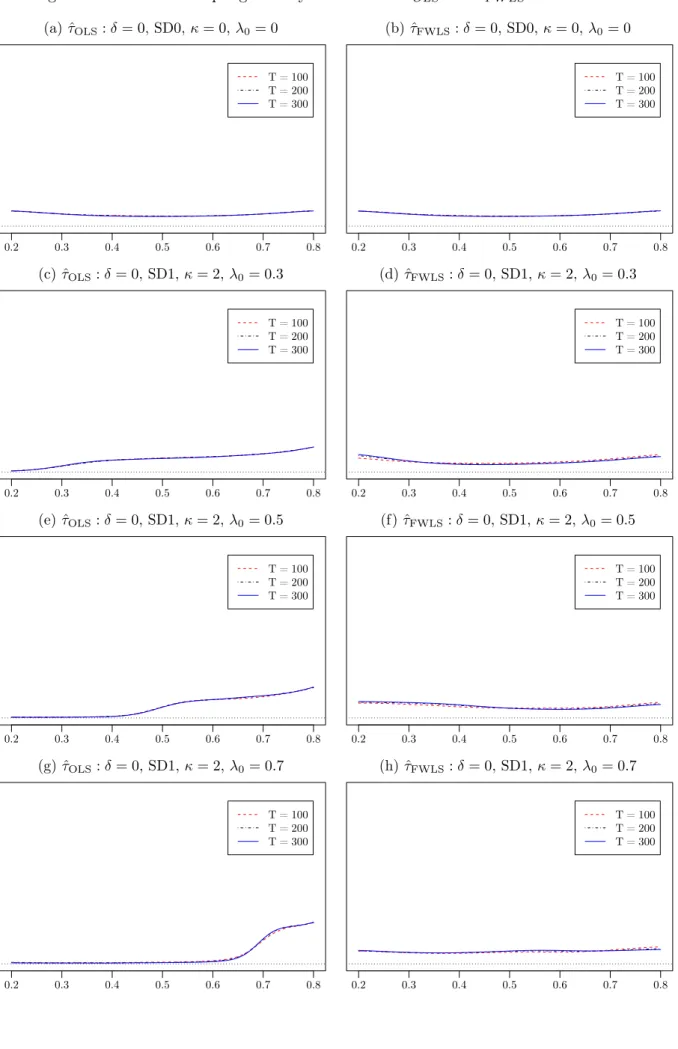
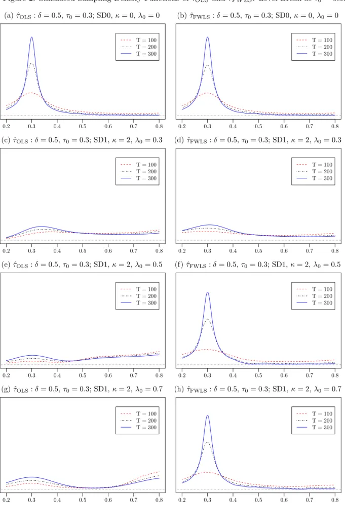
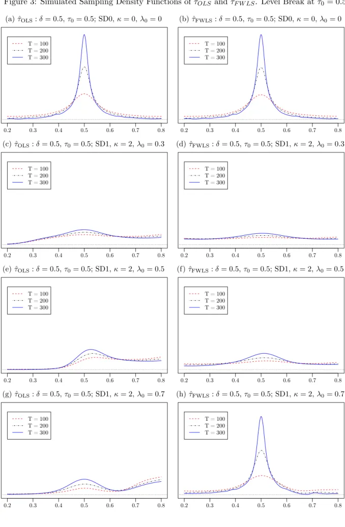
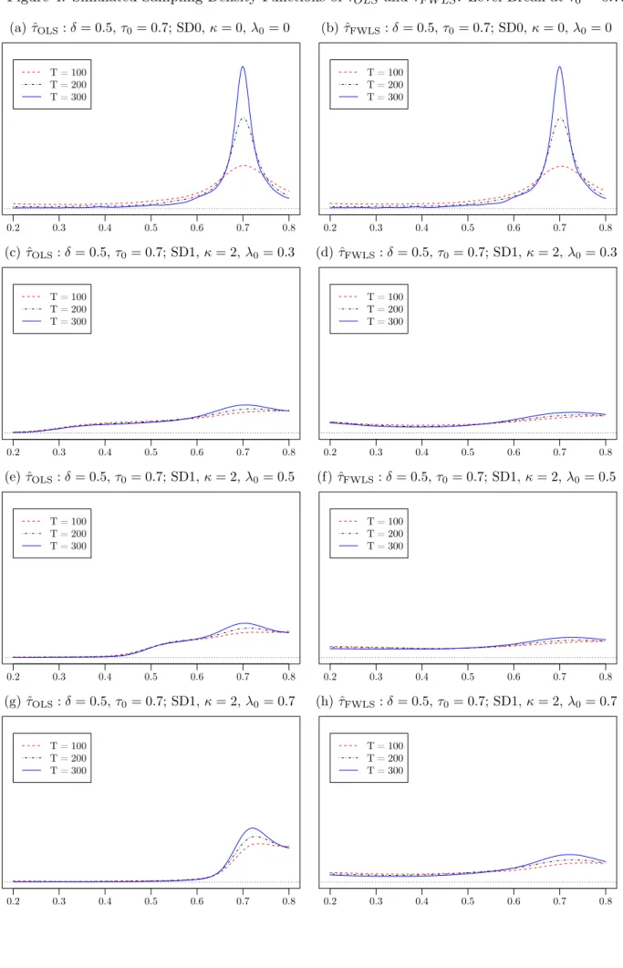
4. Figures 1-4 report corresponding plots of the empirical density functions of ˆτOLS and ˆτF W LS for samples of size 100,200 and 300 and break magnitudes δ∈ {0,0.5}, organised so that Figure 1 presents all of the results for the no level break case, while Figures 2, 3 and 4 present results for the case where a level break occurs at τ0 = 0.3, 0.5 and 0,7, respectively.
The behaviour of the ˆτOLS and ˆτF W LS estimators and the role of the heteroskedasticity and its interplay with the location of the level break location in their finite sample properties can best be revealed by considering the results in Tables 1-4 and Figures 1-4 in tandem. A consideration of all of the results presented in the tables and figures is suggestive of the basic conclusion that while both ˆτOLS and ˆτF W LS will, other things being equal, be drawn towards the location of a level break where it happens, and increasingly so as the sample size, T, and/or the break magnitude,
δ, increase, the ˆτOLS estimator is at the same time drawn towards periods of high volatility in the series, both where a level break occurs in the data and where it does not. This phenomenon is not evident in the weighted estimator, ˆτF W LS, because, by construction, ˆτF W LS down-weights the data in periods of high volatility, thereby ameliorating the tendency of the unweighted OLS break estimator to be drawn towards high volatility periods.
To illustrate these effects, consider first the results in Table 1 and Figure 1 for the case where no level break occurs, δ= 0. Here we see that for the homoskedastic case ˆτOLS and ˆτF W LS behave almost identically with a relatively uniform empirical density across the search interval with slight pile-up effects at the ends of the search set,τL= 0.2 andτU = 0.8. Both have an empirical mean of about 0.5. However, when heteroskedasticity is present the two estimators behave quite differently. While the behaviour of ˆτF W LS is seen to be relatively unchanged from the homoskedastic case in all of the heteroskedastic cases considered, the behaviour of ˆτOLS varies considerably across the different non-constant volatility cases. In particular we see that the mass of the distribution of the estimator is redistributed towards high volatility periods vis-`a-vis the homoskedastic case. This phenomenon is most obviously seen in Figure 1(g) which relates to the case where the volatility increases by a factor of 3 at λ0 = 0.7. Here we see that a large bulk of the mass of the empirical density of ˆτOLS is now spread out across the high volatility period in the data, with the empirical mean of ˆτOLS now very close to 0.8, the upper limit of the search set. In contrast, the empirical density of ˆτF W LS in Figure 1(h) is seen to be almost unchanged from the homoskedastic case. This is of course to be expected as, by construction, ˆτF W LS down-weights the data in periods of high volatility, thereby reducing the tendency of the break estimator to be drawn towards such periods. The tendency of ˆτOLS to be drawn towards high volatility periods within the data when no level break occurs has clear repercussions on the finite sample performance of ˆτOLS when a level break does occur in the data. The weighting of the data inherent in ˆτF W LS is also important for its efficacy where a level break occurs. In particular, the weighting works best in cases where the level break occurs in a low volatility period of the data, because here it down-weights the high volatility periods in the sample again reducing its tendency, relative to the OLS break estimator, to be drawn towards those periods. To illustrate this, consider Figures 2e and 2f relative to Figures 2a and 2b - in each case a level break of magnitude δ = 0.5 occurs at τ0 = 0.3. In Figures 2a and 2b, where the volatility is constant, both ˆτOLS and ˆτF W LS are centred on τ0 with the estimated densities becoming increasingly concentrated around τ0 as the sample size increases. However, in Figures
2e and 2f where the volatility increases threefold at λ0 = 0.5, although the density of ˆτF W LS is almost identical to that seen in Figure 2b, the density of ˆτOLS is radically altered. A relative peak still exists atτ0, at least for the larger sample sizes considered, but it can be observed that, as also happens when no level break is present (see Figure 1e), a large mass of the density has shifted into the high volatility region with a relative peak seen at τU = 0.8. Notice also that the performance of the ˆτOLS estimator is little improved betweenT = 100 andT = 300 here. Further illustration of these effects can also be seen from the associated results in Table 2, where the empirical mean of ˆ
τOLS is seen to be as high as 0.678 forT = 100 in this case.
The results also show that the weighted estimator is not a panacea and can in some cases display apparently inferior finite sample performance to ˆτOLS. This can occur in cases where the level break occurs in a high volatility period of the data, and especially so where the period of high volatility is short-lived. Where the level break occurs within an extended period of high volatility, weighting is relatively innocuous and there is little difference seen between ˆτOLS and ˆτF W LS. This phenomenon occurs because here, as we have already observed, some of the mass of the unweighted ˆ
τOLS estimator is attracted to the high volatility regime, regardless of whether a level break occurs or not. In contrast, ˆτF W LS down-weights the high volatility period and, as a result, where a level break occurs within the high volatility regime ˆτF W LS will have less mass in the vicinity of the level break than the ˆτOLS estimator. However, for ˆτOLS this mass will be spread across the high volatility regime and so one will still see reduced performance relative to the homoskedastic case (even where the level and volatility break locations coincide) and increasingly so the longer the duration of the high volatility period. A good illustration of this phenomenon is seen in Figures 4a-4h relating to the case where a level break occurs at τ0 = 0.7. In the homoskedastic case, ˆτOLS and ˆτF W LS perform similarly well. However, in cases where the volatility increases by a factor 3 at λ0 we see that the performance of both estimators deteriorates. For ˆτF W LS the performance is roughly similar regardless of where in the sample the volatility break occurs. For ˆτOLS the pile up of mass in the high volatility region is evident (see also Figures 1c, 1e and 1f) and so it has more mass in the vicinity of the level break - increasingly so asλ0 increases, such that the duration of the high volatility region decreases. Indeed, for the case of the longest period of high volatility where this regime starts at λ0 = 0.3 the empirical densities of ˆτOLS and ˆτF W LS are relatively similar.
We can also use the results in Figures 1-4 and Tables 1-4 to explore further how well the finite sample behaviour of ˆτOLS and ˆτF W LS conform to the predictions of the large sample theory given in Theorem 1 for level breaks of fixed magnitude and Theorem 2 for level breaks whose magnitude is local-to-zero at the Pitman rate, d= 1/2. To that end, we first recall that Theorem 1 predicts that both ˆτOLS and ˆτF W LS will be consistent for τ0 regardless of the pattern of heteroskedasticity present. Looking at the results for the constant volatility case in Table 2 and Figures 2-4 we indeed see this prediction being borne for both ˆτOLS and ˆτF W LS with each of the empirical bias, standard deviation and RMSE of the estimators decreasing, other things equal, the larger the sample size,T, for a fixed break magnitude, δ. These quantities also all decrease as the break magnitude increases while keeping the sample size constant, as anticipated by the result in Theorem 2 when d= 1/2. Moreover, as anticipated from our discussion in section 3.3, these quantities are all at their smallest when the level break occurs in the middle of the sample, i.e. τ0 = 0.5. In the heteroskedastic cases
considered, the reported results are still in general consistent with these predictions from Theorems 1 and 2 but much less obviously so.
A key prediction from Theorem 2 is that for level breaks whose magnitude is local-to-zero at the Pitman rate, the asymptotic distributions of ˆτOLS and ˆτF W LS will differ from one another, and that the form of these limiting distributions will differ for both estimators according to the pattern of unconditional heteroskedasticity present. Moreover, this large sample result also predicts that the efficacy of the two estimators will depend on the break magnitude, δ, considered relative to the parameter ω. We recall from the discussion in section 3.3 that ω provides a measure of the average volatility in the weighted data and is a function of the volatility path σ(·) and of the weighting function used (and therefore differs between ˆτOLS and ˆτF W LS). In contrast, Theorem 1 predicts that the two estimators will be identically behaved and that it is only the volatility in the neighbourhood of the level break that matters for the efficacy of the estimators. The results in Figures 1-4 and Tables 1-4 clearly demonstrate the superiority of the foregoing predictions from Theorem 2. That the finite sample behaviour of ˆτOLS and ˆτF W LS differ significantly from one another according to the form of heteroskedasticity present has already been discussed in some detail above. To illustrate the role ofω, consider Figures 2m-2p together with Table 4 which relate to the case where a level break occurs at τ0 = 0.3 and the volatility displays an upward linear trend through the sample (SD4). We can see that relative to the homoskedastic case (see Figures 2a and 2b and Table 1) the efficacy of both ˆτOLS and ˆτF W LS is considerably reduced when a trend in volatility is present, and increasingly so as the magnitude of the linear trend, κ, is increased. It is also seen that the peaks in the empirical densities at τ0 are somewhat smaller for ˆτOLS than for ˆτF W LS. Noting that ω increases as the magnitude of the linear trend increases and is higher for ˆτOLS than for ˆτF W LS3 and that the level break occurs near the start of the series (where the volatility at that point is relatively small compared to the average volatility), we clearly see that the efficacy of the estimators in finite samples is related to the average volatility across the whole sample rather than just to the volatility level near the level break, and to the weighting function used in constructing the level break fraction estimator, in each case as Theorem 2 predicts.
To illustrate further the usefulness of the asymptotic approximation provided by Theorem 2, Figure 5 provides simulations of the distribution ofQ(τ;x(·), σ(·), δ, d) with comparisons to the finite sample distributions of ˆτOLS and ˆτF W LSfrom the same DGPs. Figure 5a shows, in the broken lines, the simulated sampling distributions of ˆτOLS forT = 100,200,300 from a DGP with no level shift (δ= 0) and heteroskedasticity of the form SD2 with κ = 2 andλ0 = 0.7. The solid line shows the asymptotic approximation for this same DGP, obtained using a 2000 step discretisation. Clearly in this case the distribution of ˆτOLS is seen to be essentially the same across these sample sizes. Figure 5b shows the same information for ˆτF W LS. The asymptotic approximation remains very accurate in this case, other than a minor divergence around the time of the break in variance (λ0 = 0.7) arising from the differences of the finite sample properties of the kernel variance estimator used for finite
T and the true variance process that is used in Q(τ;x(·), σ(·), δ, d). These two figures illustrate
3
In particular, in this example the parameter ω2 = 1 whenκ = 0 (the homoskedastic case) for both ˆτOLS and
ˆ
τ(F)W LS, but for ˆτOLS,ω2 = 213 whenκ= 1 andω2 = 413 whenκ= 2, while for ˆτ(F)W LS,ω2= 2 when κ= 1 and ω2= 3 whenκ= 2.
the applicability of the stochastic component ofQ(τ;x(·), σ(·), δ, d) for predicting the finite sample behaviour of the estimators when no level shift occurs.
Figures 5c and 5d graph the simulated finite sample and asymptotic distributions when a level shift of magnitude δT = δT−1/2 at τ0 = 0.5 is included in the DGP. Both figures show that the approximation provided by the asymptotic distribution given in Theorem 2 is very accurate in cases where both a level shift and unconditional heteroskedasticity are present in the DGP. The level shift magnitude in the previous simulations was held fixed, while in this case it becomes smaller as the sample size increases. Figure 3g and 3h show the finite sample distributions with fixed level shift magnitude of 0.5, and the asymptotic approximations given in Figures 5c and 5d evidently match well with this for T = 300 in particular, since for T = 300 the implied level shift magnitude
δT = 8T−1/2 = 0.46 is close to 0.5.
The heuristic discussion of Theorem 2 given in Example 2 of Case 3 above can also be illustrated numerically. An additional simulation was carried out based on the DGP (4.1) with
σt=
(λ0(1 +κ)2+ (1−λ0))1/2
1 +κ (1 +κ·1t>bλ0Tc).
The additional scaling of σtrelative to that in Example 2 of Case 3 above is used so thatω2 = 1 for this standard deviation process for any values ofλ0 andκ, which allows meaningful comparisons to be drawn across these two parameters. In particular, simulation can be used to obtain approxima-tions to the true value of the break fraction τ0 that can be more accurately estimated from a finite sample data, based on different values of the standard deviation parameters. The analysis of the signal given in Example 2 of Case 3 above suggested that the multiplier on the deterministic signal component ofQ(τ;x(·), σ(·), δ,1/2) would be maximised at τ0= 1/2 forκ= 0 (homoskedasticity), atτ0 ≈0.19 forκ= 2 andλ0 = 0.3, and atτ0 ≈0.40 forκ= 2 andλ0 = 0.7. These calculations do not constitute formal proof that these values ofτ0 are those that can be most efficiently estimated under these variance patterns. However, the simulation results summarised in Figure 6 show that they provide a good approximation in these cases at least. Figure 6 gives plots, one for each of the three variance processes discussed here, of the simulated RMSEs of ˆτF W LS for estimating each of the indicated values of τ0 the horizontal axis, based on samples of size T = 200 and with break size δT = 8T−1/2 (i.e. the same break size considered in Figure 5 for the purposes of comparison). The values of τ0 that returned minimum RMSE of ˆτF W LS in each case were respectivelyτ0 = 0.49 (κ= 0), τ0= 0.18 (κ= 2, λ0= 0.3) and τ0 = 0.40 (κ= 2, λ0 = 0.7). Again we see that, even when used heuristically, the asymptotic approximation provided by Q(τ;x(·), σ(·), δ,1/2) in Theorem 2 provides a very useful guide to finite sample properties.
5
An Application to the Unit Root Testing Problem
We have so far demonstrated how non-stationary volatility can affect the asymptotic and finite sample properties of the OLS and (feasible) WLS estimators of the timing of a level break in time series data. However, such estimation is rarely the ultimate goal of the analysis of the time series; rather, the level break estimator is used as an input into subsequent inference. In this section we illustrate the relevance of these findings in one such important case, where the estimated level break
is used to date a trend break in a time series prior to running a unit root test. We will consider two possible scenarios which have been considered in the literature. The first, detailed in section 5.1, relates to the scenario where a trend break is known to have occurred in the data but its location is unknown to the practitioner who must therefore employ some estimate of the unknown trend break location. The second, detailed in section 5.2, relates to the empirically more relevant scenario where the practitioner neither knows whether a trend break has occurred, nor the location where it might occur. Both cases require a break date estimator, while the latter also requires some form of model selection procedure for assessing whether a break has occurred or not which can again be based on standard OLS regression estimation or on feasible WLS estimation. A Monte Carlo comparison of the relative finite sample properties of the unit root procedures based on weighted and unweighted trend break pre-tests and break fraction estimators will then be provided in section 5.3.
The underlying DGP is common to both the case where a trend break is known to have happened and where it is unknown as to whether a trend break has occurred and so we outline this first before moving to the two separate cases. To that end, consider the time series processytgenerated according to the following DGP,
yt= µ0,0+µ1,0t+zt, t= 1, . . . ,bτ0Tc µ0,1+µ1,1t+zt, t=bτ0Tc+ 1, . . . , T (5.1) where zt=φTzt−1+et, (5.2)
and where et is generated according to (2.2) and is again taken to satisfy the conditions of As-sumption A. As is common in this literature, we also assume that the initial condition satisfies
T−1/2z0 p
→0. This latter condition can be weakened, but at the expense of additional complexity. In (5.2) we will follow the convention in the unit root testing literature and focus on the near-integrated autoregressive model, Hc : φT := 1 +c/T with −∞ < c ≤ 0. We will therefore be concerned with testing the unit root null hypothesis, H0 : c = 0, against local alternatives, Hc where c <0.
In the context of the observation equation in (5.1), yt has a linear trend with break in both intercept and slope occurring at time bτ0Tc. Following Harris et al. (2009) and Cavaliere et al. (2011), among others, we will focus on the situation where the trend function is restricted to be continuous at the break point, so that the coefficients satisfy µ0,0+µ1,0bτ0Tc=µ0,1+µ1,1bτ0Tc. In this case the trend specification can be written as4
yt=α+µt+δT1t>bτ0Tc(t− bτ0Tc) +zt (5.3)
with α:=µ0,0,µ:=µ1,0 and δT :=µ1,1−µ1,0 (allowing for the magnitude of the break to depend on T as the previous sections). Taking first differences we obtain
∆yt=µ+δT1t>bτ0Tc+ ∆zt, (5.4) 4
The imposition of continuity on the trend function makes the connection to the level shift results clear and simple. The restriction is not compulsory, however, as without it the equation corresponding to (5.4) would be given by ∆yt =µ+λ1t=bτ0Tc+γ1t>bτ0Tc+ ∆zt, and the effect of the additional impulse dummy variable 1t=b0 is
where ∆ := (1−L) denotes the first difference operator. Under the unit root null hypothesis,H0, (5.4) can be seen to coincide with (2.1) on replacing yt by ∆yt in the latter. Consequently, the results obtained in section 3 relating to the estimation of the level break location therefore continue to apply in this context, so that we estimate the trend break location via level break estimation applied to the first differences of the data.
5.1 The Case Where a Trend Break is Known to Have Occurred
In this first scenario we consider, the practitioner knows that the trend break magnitude δ is non-zero, but does not know the true location, τ0, of the trend break.
We will base our unit root test on Dickey-Fuller [DF] type statistics which model the trend break. These statistics are based on a two step procedure whereby the data are de-trended in the first step and in the second step a standard DF test is applied to the de-trended data. We will follow the recent literature and use the quasi-difference [QD] de-trending approach of Elliott et al.
(1996) in what follows although OLS de-trending could alternatively be used. For a generic trend break location, τ, the QD de-trended data are given by ˆzτ,t := yt−Xt(τ)0θˆc¯, where Xt(τ) :=
1, t, (t− bT τc)·1t>bT τc 0
and ˆθ¯c the vector of OLS parameter estimates from the regression of
yc,t¯ on X¯c,t(τ), with y¯c,1 := y1, y¯c,t := yt−φ¯Tyt−1, t = 2, ..., T; X¯c,1(τ) := X1(τ), Xc,t¯ (τ) :=
Xt(τ)−φ¯TXt−1(τ), t = 2, . . . , T, and where ¯φT := 1 + ¯c/T , where ¯c is the QD parameter. The QD de-trended data ˆzτ,t can then be used to estimate the DF regression
ˆ
zτ,t = ˆφτzˆτ,t−1+ ˆeτ,t (5.5) and hence to obtain the usual DF t-statistic
tτ := ˆ
φτ −1 s.e( ˆφτ)
. (5.6)
Theorem 4 provides the limiting distribution under the local alternative Hc of tτ when evaluated at the true break fraction τ = τ0. The theorem also shows that this limit is unchanged when τ0 is replaced by either the OLS break fraction estimate, ˆτOLS, or the corresponding feasible WLS estimate, ˆτF W LS. We will use the simplified notationtOLS and tF W LS for the DF tests based on ˆ
τOLS and ˆτF W LS, respectively, in what follows.
Theorem 4. Let yt be generated according to (5.1)-(5.2)and with et generated according to (2.2),
and let the conditions of Assumption A hold. Let δT =δT−d, d≥0. Then, under Hc:
(i) For any d≥0, and regardless of whether δ= 0 or δ6= 0,
tτ0 d → 1 2(Z(1;τ0, c,¯c, η) 2−1) R1 0 Z(s;τ0, c, η)2ds 1/2 :=ξ(τ0, c,¯c, η) (5.7) where Z(s;τ, c,c, η¯ ) :=Bηc(s)−X(s;τ)0 Z 1 0 X¯c(s;τ)X¯c(s;τ)0ds −1Z 1 0 X¯c(s;τ)dBηc(s; ¯c)
and Bηc(s) := Z s 0 exp(c(s−r))dBη(r), Bηc(s; ¯c) :=Bηc(s)−c¯ Z s 0 Bηc(r)dr, with Bc
η(·) as defined in Theorem 2, and
X(s;τ) := s (s−τ)∨0 ! , Xc¯(s;τ) := 1−¯cs 1−¯c((s−τ)∨0) ! .
(ii) For 0≤d <1/2, and providedδ 6= 0, it holds that: (a) tOLS −tτ0
p
→0, and (b) provided the additional conditions of Theorem 3 hold, tF W LS−tτ0
p
→0.
Remark 5.1. The results in Theorem 4 and in what follows will continue to hold in the case where
et admits serial correlation of the form outlined in Remark 3.2. Under the standard invertibility condition on C(L) thatC(z)6= 0 for all|z| ≤1, the serial correlation in et can be captured in the usual way using an augmented Dickey-Fuller [ADF] statistic, whereby (5.5) is augmented by the addition of the lagged dependent variables, {∆yt−j}pj=1, where p satisfies the usual rate condition
that 1/p+p3/T →0, as T → ∞.
Remark 5.2. The results in part (ii) of Theorem 4 might appear to contradict with Proposition 3 of Kim and Perron (2009,p.12) where it is shown that for some generic break fraction estimator, ˜τ, the break fraction, τ0 must be consistently estimated at some rate greater thanT1/2 in order for a DF test based on ˜τ,tτ˜say, andtτ0 to be asymptotically equivalent. However, the result in Kim and
Perron (2009) relates only to the case where the trend break magnitude δT is fixed and non-zero (see their Assumption 1 on page 3), and therefore corresponds to the specific case ofd= 0 andδ6= 0 in Theorem 4. In this case we know from Theorem 1 that both ˆτOLS and ˆτF W LS are consistent at rate Op(T−1), which certainly satisfies the condition in Proposition 3 of Kim and Perron (2009, p.4). In the more general set-up we consider here, the trend break magnitude and convergence rate of ˆτOLS and ˆτF W LS change together; as the break magnitude slows, so commensurately does the convergence rate of ˆτOLS,τˆF W LS. In particular, where the trend break magnitude is of orderT−d,
d≥0, then, as shown in Theorems 1 and 3, respectively, (ˆτOLS−τ0) and (ˆτF W LS−τ0) are both of
Op(T2d−1). However, this rate of consistency is still sufficiently fast for the asymptotic equivalence results in part (ii) of Theorem 4 to hold, precisely because the magnitude of the trend break is
shrinking commensurately with the reduced consistency rate.
Remark 5.3. The result in Theorem 4 relates to the “large” break case of section 3.2 where 0≤d <1/2 in the localisation of the trend break magnitude, such that the trend break locationτ0 can be consistently estimated. Localisations which converge to zero at a faster rate, as considered in section 3.3, including the Pitman drift rate where d= 1/2, are excluded. Our aim in this section is not to provide a comprehensive treatment of the large sample properties of unit root tests in the present setting but rather to show how weighted trend break estimators can improve the finite sample properties of unit root tests relative to standard OLS estimation. However, the results could be extended to cover the case of d ≥ 1/2. For d = 1/2, results comparable to those given in section 5 of Harvey et al. (2012), but generalised by the non-stationary volatility allowed for under Assumption A2, would be obtained. For d > 1/2, as discussed in Case 1 in section 3.3, the