Improving Business Cycle Forecasts’ Accuracy - What Can We Learn from Past Errors?

(1)

Roland Döhrn

What Can We Learn from Past Errors?

No. 51

RWI

ESSEN

R

W

I:

Discussion

P

apers

(2)

für Wirtschaftsforschung

Board of Directors:

Prof. Dr. Christoph M. Schmidt, Ph.D. (President), Prof. Dr. Thomas K. Bauer

Prof. Dr. Wim Kösters Governing Board:

Dr. Eberhard Heinke (Chairman);

Dr. Dietmar Kuhnt, Dr. Henning Osthues-Albrecht, Reinhold Schulte (Vice Chairmen);

Prof. Dr.-Ing. Dieter Ameling, Manfred Breuer, Christoph Dänzer-Vanotti, Dr. Hans Georg Fabritius, Prof. Dr. Harald B. Giesel, Dr. Thomas Köster, Heinz Krommen, Tillmann Neinhaus, Dr. Torsten Schmidt, Dr. Gerd Willamowski Advisory Board:

Prof. David Card, Ph.D., Prof. Dr. Clemens Fuest, Prof. Dr. Walter Krämer, Prof. Dr. Michael Lechner, Prof. Dr. Till Requate, Prof. Nina Smith, Ph.D., Prof. Dr. Harald Uhlig, Prof. Dr. Josef Zweimüller

Honorary Members of RWI Essen

Heinrich Frommknecht, Prof. Dr. Paul Klemmer †

RWI : Discussion Papers

No. 51

Editor: Prof. Dr. Christoph M. Schmidt, Ph.D. ISSN 1612-3565 – ISBN 3-936454-78-7 ISBN-13 978-3-936454-78-9

The working papers published in the Series constitute work in progress circulated to stimulate discussion and critical comments. Views expressed represent exclusively the authors’ own opinions and do not necessarily reflect those of the RWI Essen.

(3)

RWI : Discussion Papers

No. 51

Roland Döhrn

RWI

ESSEN

(4)

Nationalbibliografie; detaillierte bibliografische Daten sind im Internet über http://dnb.ddb.de abrufbar.

ISSN 1612-3565 ISBN 3-936454-78-7 ISBN-13 978-3-936454-78-9

(5)

Roland Döhrn*

Improving Business Cycle Forecasts’ Accuracy –

What Can We Learn from Past Errors?

Abstract

This paper addresses the question whether forecasters could have been able to produce better forecasts by using the available information more efficiently (informational efficiency of forecast). It is tested whether forecast errors covariate with indicators such as survey results, monetary data, business cycle indicators, or financial data. Because of the short sampling period and data problems, a non parametric ranked sign test is applied. The analysis is carried out for GDP and its main components. The study differentiates between two types of errors: Type I error occurs when forecasters neglect the information provided by an indicator. As type II error a situation is labelled in which fore-casters have given too much weight to an indicator. In a number of cases forecast errors and the indicators are correlated, though mostly at a rather low level of significance. In most cases type I errors have been found. Additional tests reveal that there is little evidence of institution specific as well as forecast horizon specific effects. In many cases, co-variations found for GDP are not refected in one of the expenditure side components et vice versa.

JEL classification: E370, C530, C420

Keywords: Short term forecast, Forecast evaluation, informational efficiency October 2006

*Roland Döhrn, RWI Essen, Germany. Revised paper presented at the International Symposium of Forecasters June 2006 11 to 14 in Santander, Spain. The author would like to thank György Barabas, Torge Middendorf, Torsten Schmidt, and Wim Kösters for helpful comments to earlier versions of this paper. All correspondence to Roland Döhrn, Rheinisch-Westfälisches Institut für Wirtschaftsforschung (RWI Essen), Hohenzollernstr. 1–3, 45128 Essen, Germany, Fax: +49 201 / 81 49-200. Email: [email protected].

(6)

1. Background and Structure of the Paper

Evaluating forecasts is an exercise which is done more or less regularly by pro-ducers of business cycle forecasts as well as independent researchers. Re-viewing recent literature on this issue, the papers aim at quite different di-rections. Some primarily take the users’ view and present implicitly a ranking of different forecasts with respect to their accuracy (e.g. Öller, Barot 2000). Other analyses try to detect common features from various forecasts by dif-ferent institutions (Rouss, Savioz 2002; Döpke, Fritzsche 2005). A difdif-ferent strand of research comes from institutions evaluating the accuracy of their own forecasts often employing a wide spectrum of statistical measures (Keereman 1999; Kontsogeorgopoulos 2000; Timmermann 2006). Finally, only few researchers try to gather hints from past forecast errors, how to improve future forecasts (for Germany e.g. Neumann, Buscher 1985; Kirchgässner, Savioz 2001; for the U.S. Steckler 2002: 232–233 gives an overview).

This paper tries to add some new evidence to the last category from a fore-caster’s perspective. For that purpose, some short term forecasts for the German economy the author of the paper is engaged in are analysed. In par-ticular it is asked whether a broad set of information available at the time of the projection has been used properly. This issue is addressed as one aspect of informational efficiency of forecasts in the forecast evaluation literature. Various tests for informational efficiency are proposed having one feature in common: They analyse forecast errors with respect to their correlation with past data supposed to contain information about future economic devel-opments and presumably have been known to the forecaster when he made his prediction. If errors are uncorrelated with such variables, it can be assumed that the accuracy of the forecast could not have been improved by making a better use of these data. If the opposite is true, there should be reason to check, whether the data in question could have been utilised better.

As far as this kind of analyses has been carried out earlier the focus mostly was on GDP forecasts. However, it must be taken into account how short term forecasts are made in practice. Without going into detail, they are mostly built bottom-up, starting with forecast of the expenditure side of GDP at a disaggregated level. These detailed forecasts are added up to yield a GDP forecast, which, however, may be subject to some fine tuning thereafter. Therefore it would help little to improve predictions if a correlation is de-tected between some economic indicators and the errors of GDP forecasts. If, e.g., it turns out that the error in GDP forecast and share prices are correlated, a forecaster would not know whether he failed in assessing the wealth effect, which would require to scrutinize consumption forecast, or whether he did not take into account properly the impact of share prices on financing conditions and, thus, on investment. Therefore, this paper also takes into account the

(7)

in-formational efficiency of forecasts of the expenditure side components of GDP.

The paper is organised as follows: In section 2, the concept of informational ef-ficiency of forecasts is discussed and the method employed in this paper is de-scribed. Section 3 provides some details about the forecasts considered and gives some measures of their accuracy. Furthermore the short term indicators are described. In Section 4, the results of the tests for information accuracy are presented. The final section offers some conclusions.

2. Methodology

2.1 Concepts of Informational Efficiency

Several measures to evaluate forecast efficiency are proposed in literature. A simple test is the so called Mincer-Zarnowitz equation, which regresses the re-alized rate of growthrof a variable on the predicted change fof the same variable

(1) rt=α0+α1⋅ +ft εt.

εt is an error term which is assumed to be normally distributed with mean zero. In an efficient forecast (“Mincer-Zarnowitz-efficiency”),α₀ should be equal to 0 andα₁equal to 1, which can be tested by an F-test. In caseα₁ is above 1, the forecaster is “timid”, i.e. he underestimates high and overestimates low growth rates: The opposite applies ifα₁ is lower than 1. Ifα₀ differs from 0 whileα₁ equals 1, the forecast is biased.

For a stronger test for informational efficiency, various extensions of the Mincer-Zarnowitz equation are proposed. One approach is to enclosert−1 as

an additional explanatory variable

(2) rt =α0+α1⋅ +ft α2 ⋅rt−1+εt.

Ifα₂ differs from zero significantly, the forecast tends to covariate with the last observation. Ifα₂ is negative, the forecast is systematically too optimistic in years following a “good” year and over-pessimistic in those following “bad” years. In the caseα₂ is positive the opposite applies. In a more direct testr_t₋₁is replaced by other data xt which have been known by the forecaster when making his prediction.

(3) r_t =α₀+α₁⋅ +f_t α₂ ⋅x_{i t}_,₋₁+ε_t.

Whether the factors included in (2) and (3) do really improve a forecast can be tested in different ways. Stekler (2002: 224) proposes the null hypothesis

(8)

α2 =0, which can be tested by a simple t-test. Holden/Peel (1990) suggest the

null hypothesisα₀ =0,α₁=1andα₂ =0and to apply an F-test instead.

2.2 A Non-parametric Test

However, these tests might be inappropriate in the case at hand for various reasons. First of all, the number of observations is rather small here, so that the results of the test may be spurious. This problem is aggravated by the fact that in short term forecasts the total error typically can be attributed to a rather small number of cases in which forecast errors are extraordinary large. Therefore it may be more appropriate to employ non-parametric tests as e.g. a sign test which has been suggested for similar applications (e.g. forecast com-parisons; Diebold, Mariano 1999: 392). A less sophisticated testing technique may also be suitable because of the quality of the data: On the one hand, real time data for the indicatorsxwould be required to get a adequate picture of the forecaster’s information background. These are, however, hard to collect for many indicators. On the other hand, the forecast errors measured can only be approximations of the “true” error, because many institutions rounded off their forecast values to 0.5 percentage points until the late 1990s.

Therefore the subsequent analyses will be based on a non-parametric test which has been proposed by Campbell/Ghysels (1995). In the following the forecast errors will be denoted as

(4) et = −ft rt.

As the test is based on the number of positive signs ofe, it can only be applied for unbiased forecasts. Therefore, a sign test for unbiasedness will be applied at first whether the median forecast is 0

(5) S I et t =

∑

+( ) where: I et e t + = > ⎧ ⎨ ⎩ ( ) 1 0 0 if otherwise.

Sis cumulative binominal distributed with probability 0.5. In our case (n=14 ,) unbiasedness must be rejected in a two tailed test on a 10% level, if the number of positive signs is not larger than 3 or above 11 (5%: 2 or 12; 1%: 1 or 13). To take into account a potential bias,e_twill be corrected subsequently by subtracting the median bias

(6) et e median e e e

c

t t n t n t

(9)

There is a further reason why (3) may lead to wrong results when it is applied in a way widely used. In the estimate the entire sample of forecast errors and indicators is used. But this is not the typical situation a forecaster is in: In periodthe only knows thet−1,t−2Kobservations. In the regression, also the

t+1,t+2Kdata are used. Therefore, the test for informational efficiency as de-scribed in (3) may be misleading. To avoid this problem here, the x will be “normalised” with respect to past data. Campbell/Ghysels (1995) propose in this context to subtract the median ofxin the most recentkyears fromx. The transformation is similar to (6)

(7) xt k x median x x x

c

t t k t k t

, = − ( − , − +1,K, ).

Ifxfollows a clear upward (downward) trend, this transformation could result inxc

being positive (negative) in most cases. Therefore the x must be trans-formed in a way making the indicators stationary. Subsequently in the case of non-stationary indicators, their growth rates will be used to conduct the test. Having done this, the orthogonality test for independence ofeandxcan be based on a rather simple statistic

(8) z_tk e x

t t k c

= ⋅ , .

Defining I+ in the same way as in (5), a first test statistic can be calculated as:

(9) SO I zt

k t

=

∑

+( ).

It is cumulative binominal distributed with probability 0.5. The critical values are the same as cited before.

The sign test requires rather weak assumptions only, but it is on the other hand also a rather weak test. If errors are distributed symmetrically, a ranked sign test can be applied which was proposed by Campbell/Ghysels (1995: 23–24)1_.

In this test, the absolute forecast errors are ranked, and the ranks are used as weights for the signs in (9)

(10) WO I zt rank e

k

t t

=

∑

+( )⋅ (| |).

WOis Wilcoxon rank signed distributed. For small samples, the critical values can be taken from special tables (e.g. Siegel 1956: 254). In the present case of 14 observations the hypothesis thatxt k, andet are independent must be re-jected on a 10%-level when the sum of positive ranks is above 80 or below 25 (5%: 84 and 21; 1%: 92 and 13) in a two tailed test. For large samples, the

Improving Business Cycle Forecasts’ Accuracy 7

(10)

Gaussian distribution can be applied after having standardizedWO2_{. In the}

present case, the critical values calculated from the Gaussian distribution differ little from those taken from the tables. As the application of the Gaussian distribution makes it easier to conduct a large number of tests, it will be applied here.

2.3 Type I and Type II Errors

When using data to make a prediction, forecasters may be wrong in two ways. Firstly, they may neglect some indicators that would be useful for the forecast, or they underestimate their influence (type I error). Secondly, they may put too much emphasis on an indicator (type II error). These two cases will be il-lustrated by an example: If business surveys indicate more optimistic expec-tations in the manufacturing sector (xt

c

is positive), some forecasters may revise their prediction on GDP upward, some not. After GDP figures being published, and having compared forecasts with realisation it may turn out, that some forecasters may have been too pessimistic, because they did not suffi-ciently pay attention to the business expectation index. In the terminology used here, they made a type I error. If this happened several times in the past, forecast errors tend to be negative whenever business expectations improved. Hence, a type I error would show up in low values ofWO. Some forecasters, on the other hand, may overdue. They may take any indication that expectations improve to revise their forecast upward, what in the rear view may turn out to be over-optimistic. That is the typical case of the type II error. It will lead to high values ofWO. To be able to distinguish these two cases, allxc

variables in this study will be standardized in a way that positive (negative) values van be interpreted as indicators of high (low) growth rates.

3. Data Description

3.1 Forecasts Analysed

Subsequently the information efficiency of the forecasts produced by RWI Essen and theGemeinschaftsdiagnose(GD) will be tested. Both predictions are outcomes of a national accounts based iterative forecasting procedure, which allows integrating various forecasting techniques. Hence it is not clear, what role the indicators considered later play in the end in making these forecasts. Therefore, this kind of forecast is highly suitable for the analyses carried out here.

2 The mean of the Wilcoxon test statistic with n observations is (n+1) /4 and its variance

n n( ₊1 2)( n₊1) /24. In the literature different thresholds can be found to mark whether a sample is large.

(11)

RWI Essen publishes a GDP forecast twice a year, in February and July3_,

pro-viding predictions for the current and for the next year (RWI : Konjunktur-berichte). The February report contains a forecast for the next year only since 1998. Therefore, the forecast published in February for the following year cannot be analysed here due to an insufficient number of observations. The July forecast has a horizon of 7 quarters. All in all, three forecasts per year can be analysed subsequent. They are named according to their forecast horizon in terms of quarterly GDP figures to be projected:

– The July forecast for the following year with a horizon of 7 quarters (RWI-7),

– the February prediction of the current year with a horizon of 4 quarters (RWI-4), and finally

– the July forecast of the current year with an horizon of 3 quarters (RWI-3). The forecast of the GD is a result of the joint effort of six (up to 1993 five) leading German economic research institutes (Arbeitsgemeinschaft, var. years), one of them being RWI Essen. It is commissioned by the Federal Ministry of Economics and published twice a year, in April and October. In April it comprises a forecast horizon of 8 (before 1997 of 4) quarters, the first quarter of the current year being still a forecast, in October the forecast period is 6 quarters. Again, the April forecast for the next year does not offer a suf-ficient number of data. Therefore, three forecasts from the GD can be analysed in this study:

– The October forecasts for the following year with a horizon of 6 quarters (GD-6),

– Those issued in April of the current year with a forecast horizon of 4 quar-ters (GD-4).

– Finally, the October forecasts for the current year with a horizon of 2 quar-ters (GD-2).

From a statistical point of view, it is desirable to analyse forecast accuracy over a long period to have a sufficient number of observations. However, the meth-odology as well as the data background of the forecasts underwent consid-erable changes over the last decades. National accounts data as well as many business cycle indicators are published more up to date today than they have been in the past. Furthermore, forecast methods as well as the personal and professional background of the forecasters might have changed. An analysis over a very long period could be spoilt by these factors too much. Hence, this

3 For the RWI forecast the publication date varies to some extent, but in each year it includes the data for the same number of quarters from the national accounts. The flash forecast for the year ahead published in December will be neglected subsequently, as it did not differ substantially from the February forecast.

(12)

paper is restricted to the years after 1991, taking the German unification as a “natural” break. From 1991 to 1994 forecasts for Western Germany only and thereafter for the unified Germany are considered. The sample period ends 2004.

National accounts data are often revised quite substantially after the first pub-lication (Braakmann 2003; Öller, Hansson 2002). Therefore it is difficult to de-termine what figures should serve as “realisations” to compare the forecast with. In the following, the first published quarterly national accounts are taken as a yardstick. This procedure has been employed in other forecast evaluations too (e.g. Kirchgässner, Savioz 2001: 358). It seems plausible since the first “of-ficial” data are based mostly on the information which also forms the back-ground of the forecast. Later revisions may be substantial, but they hardly could have been anticipated, in particular if they emerge from new definitions in the national accounts or from changed methods to compile data.

Table 1 compares some measures of forecast accuracy of the six GDP forecasts under scrutiny with a sample of other projections, partly from international in-stitutions. It shows that the Mean Absolute Forecasting Error (MAFE) as well as the Mean Squared Forecasting Error (MSFE) and the BIAS do not differ to much from the values calculated for other forecasts published at the same time. Hence, the predictions analysed here seem to be state of the art.

Accuracy of Forecasts of Annual GDP Growth in Germany

1991–2004 Institution Forecast horizon (quarters) Month published Mean Absolute Forecasting Error (MAFE) Mean Squared Forecasting Error (MSFE) BIAS RWI (RWI-7) 7 July 1.26 2.87 1.03

IMF 6 September 1.22 2.93 0.96 GD (GD-6) 6 October 0.99 1.47 0.64 Sachverständigenrat 6 November 0.84 1.17 0.47 EU 6 November 0.91 1.32 0.56 OECD 6 December 0.92 1.35 0.45 Jahreswirtschaftsbericht 5 January 0.75 0.90 0.49 RWI (RWI-4) 4 February 0.76 0.98 0.54

IMF 4 April 0.53 0.45 0.11

GD (GD-4) 4 April 0.57 0.48 0.09

EU 3 May 0.55 0.50 0.11

OECD 3 June 0.49 0.45 0.06

RWI (RWI-3) 3 July 0.40 0.30 0.16 GD (GD-2) 2 October 0.17 0.04 0.05 Author’s computations.

(13)

As already noted, short term predictions are mostly made bottom up. Even if in the very short run (1–2 quarters) the sectoral production forecasts also may play an important role, in the end the forecasts are dominated by projections of the demand side of GDP. Therefore, in addition to GDP also the efficiency of forecasts of the demand categories will be analysed. Attention will be paid to private (PC) and public consumption expenditure (GC), investment in equipment (IEQ) and structures (IS), and, finally, exports (EX) and imports (IM).

Table 2 presents some statistics of the accuracy of the demand side forecasts, taking the RWI-4 and GD-4 forecasts as examples. It clearly can be seen that the accuracy of the GDP forecast is owed to compensating errors: For almost each component, government consumption being the only exception, the forecast error is by far larger than that for GDP. Investment in equipment shows the largest error, and the forecasts are markedly biased upward. Large errors also occur in export and import forecasts. The somewhat better per-formance of GD-4 compared to RWI-4 is partly owed to the fact that the first is published at a minimum of 4 weeks later than the second which allows to make use of additional information helping to improve accuracy.

3.2 Short Term Indicators Employed

There is no clear rule at hand, which short term indicators should be employed in the tests to follow. As a rule, forecasters use many data for their work. Therefore, numerous variables could be tested whether they were used effi-ciently and a selection has to be made to restrict the scope of the further analysis. Subsequently five types of variables will be considered (for a detailed documentation of the indicators see annex.):

– Economic sentiment variables: Three indicators will be used: ifo business cli-mate (IFOC), ifo business expectations (IFOE) and the consumer

senti-Improving Business Cycle Forecasts’ Accuracy 11

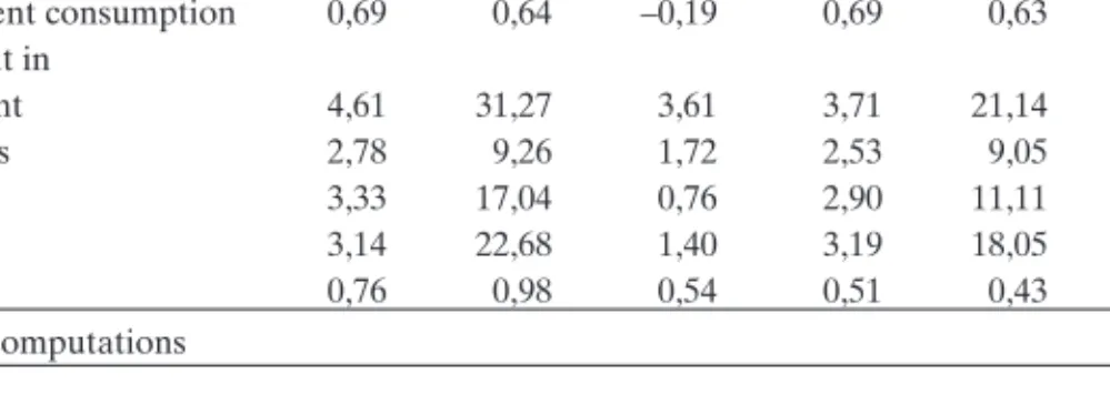
Accuracy of RWI-4 and GD-4 Forecasts of the Annual Growth of GDP Components

1991–2004

RWI-4 GD-4

MAFE MSFE BIAS MAFE MSFE BIAS Private consumption 0,91 1,12 0,61 0,71 0,75 0,30 Government consumption 0,69 0,64 –0,19 0,69 0,63 –0,20 Investment in equipment 4,61 31,27 3,61 3,71 21,14 2,46 structures 2,78 9,26 1,72 2,53 9,05 0,84 Export 3,33 17,04 0,76 2,90 11,11 0,03 Import 3,14 22,68 1,40 3,19 18,05 1,11 GDP 0,76 0,98 0,54 0,51 0,43 0,11 Author’s computations Table 2

(14)

ment index (CSI) which is published by the European Commission. IFOC and IFOE are available during the last week of each month presenting the results for current month. For our test it is assumed that the forecasters know the data of the month before their forecast is published. The CSI is is-sued with a longer lag. It is assumed forecasters know the result of the last but one month. For forecasts published in July, e.g., the May CSI is included in our test.

– Three variants of leading indicatorsfrom official sources are considered: Total (NOMT) as well as foreign new orders in manufacturing (NOMF) are published by the German statistical office approximately 6 weeks after the end of the month the data were collected. New orders in construction (NOC) are issued about 2 weeks later. When forecasters issue their July forecast, they know the May data on orderbooks as a rule. As there are huge short term fluctuations in the data sometimes, they are smoothed by calcu-lating two month averages of seasonal adjusted indicators. Using month over month changes makes sure that the data are stationary.

– Various interest rates as well as the real effective exchange rate are consid-ered asmonetary variables. These data are available very shortly after the end of a month. Therefore averages of the rates for the month before the forecast is published are included in the analysis. Thus, the yield curve (YC = long term rate LR minus short term rate SR), and the real short term rate (RSR) as an indicator of monetary policy stance. As monetary policy often shows its impact with long lags, also averages of the short term (SR-1) , the long term (LR-1), and the real short term interest rate (RSR-1) as well as of the yield curve (YC-1) over the entire year before the forecast are intro-duced into our calculations. Kirchgässner/Savioz (2001) found a correlation between forecast errors and interest rates when they tested for such long lags4_{. As the interest rates are already stationary, no transformation is}

re-quired. Furthermore the real effective exchange rate is included as a mone-tary indicator, in two variants: the year over year change in the last month (REER) as well as of the average of the last three months (REER3).

– Asfinancial market indicatorsshare price index CDAX is included in our study. Again, two transformations are tested: Firstly, the year over year change in the month before the forecast (CDAX) is published, secondly the change of the three previous months (CDAX3).

– Finally, the OECD composite leading indicator (OECD) is tested. It com-bines various data already considered here, namely the ifo business climate (IFOC) and total new orders in manufacturing (NOMT) with financial data (YC) and additional information taken from the ifo business survey (OECD 2002: 31).

4 We refrained from including monetary aggregates such as M3 into the calculations as there is a break in the time series due to the start of EMU.

(15)

All these indicators are available at least back to 1979, CSI being the only ex-ception (since 1985). The calculate the “centered” indicators according to (7), the median of the observations over the last 10 years is subtracted from the figure included in the test; the median has been calculated for monthly data. Before 1991 West German data have been used, thereafter data for unified Germany.

4. Results of the Tests

In a first step it is tested whether the forecasts considered are unbiased (table 3). As this is not the case in particular for the projections with longer ho-rizons and for most of the forecasts of private consumption expenditure (PC), the correction described in (6) has been applied to all forecasts. After this transformation the rank signed test is calculated.

Table 4 summarizes the results of the orthogonality test. In 100 out of 798 com-binations of indicators, economic aggregates and forecasts co-variation was found which was significant at least at a 10%-level. Before making reference to specific results, some more general conclusions can be presented first:

– In many cases (45 out of 100) a co-variation between forecast errors and economic indicators is significant at a 10%-level only, giving a rather weak indication for possibilities to improve forecasts.

– There is no indication that the two forecasters exploit the data in a different way; in 44 cases a co-variation of indicators with the RWI forecast errors was found, in 56 cases with the GD forecast errors.χ2

shows that the differ-ences are not significant.

– Comparing forecasts of different horizons, a closer look at the indicators might help to improve the forecasts with a 4 months horizon in particular (40 cases). A smaller number of significant correlations was found for the forecast with longer (RWI-7, GD-6: 29 cases) as well with a shorter horizon (RWI-3, GD-4: 31 cases).

– Most correlations (30) are observed with errors in GDP forecasts. On the other hand, only in 6 cases errors in investment in struktures forecasts covariate significantly with any of the indicators considered. For goverment consuption the number of correlations is quite small (9), too. For invest-ment in equipinvest-ment, which is the forecast with the highest average error, 15 cases of significant correlations are observed.

– If a correlation is detected between an indicator and GDP, the same indica-tor as a rule does not covariate with one of the demand side components of GDP et vice versa.

– Type I errors (72 out of 100) predominate, i.e. forecasters make insufficient use of some indicators. On the other hand, they over-estimate the impact of

(16)

the indicators only in a few cases. In the RWI forecasts the type II error is more common (21 cases) than in the GD forecasts.

Addressing some specific findings, an outstanding result is the strong corre-lation of changes in the OECD leading indicator with errors of the forecasts with relative long horizons, in particular the GD-6 forecast. Indeed, OECD (2002: 33) shows in hindsight that some turning points in the business cycle were indicated by the OECD index with a rather long lead in the 1990s. This was particularly true for the start of the downturn in 1992 and the recovery in 1993. The forecasters obviously were not aware of these interrelations in the past. But surprisingly the result for GDP is not mirrored in any of the GDP components.

One important source for calculating the OECD leading indicator is the ifo business survey. Therefore, it is not very surprising that forecast errors also covariate with ifo business expectations. However, it is a bit surprising that the survey contains some information that might help to improve even the GD-6 forecast, because the companies were asked to assess their expectation over the next six months only. But again, this interrelation is not mirrored in the components of GDP.

Finally, a strong correlation is also found between errors in the GDP forecast of GD-4 and GD-2 on the one hand and share prices on the other hand. At least in GD-4 the forecast error of exports also shows some co-variation with changes in share prices. Other channels through which the share market can be expected to influence GDP growth seem to have been taken into account correctly: Neither private consumption expenditure nor investment in equipment show any interrelation.

Test for BIAS of the Forecasts Considered1

1991–2004, S-values and their level of significance

RWI-7 RWI-4 RWI-3 GD-6 GD-4 GD-2

GDP 12** 10 8 10 7 8

Private consumption (PC) 12** 12** 10 12** 10 7 Government consumption (GC) 7 6 5 5 6 2** Investment in equipment (IEQ) 11* 11* 11* 10 9 9 Investment in structures (IS) 10 11* 9 10 10 6

Exports (EX) 9 8 8 8 5 6

Imports (IM) 9 8 9 8 7 9

Author's computations. –1See eq. (8). For abbreviations see tables 1. Level of significance: *** 1%; ** 5%; * 10%.

(17)

Test for Information Efficiency Based on a Ranked Sign Test1

1991–2004

Indicator RWI-7 RWI-4 RWI-3 GD-6 GD-4 GD-2 ifo business expectations

(IFOE) GDP 20,5** 4*** 15,5** 21** PC 20** GC IEQ 81* IS EX IM ifo business climate

(IFOC) GDP 25,5* PC 17,5** 21,5* GC 20** IEQ 89** 24,5* IS EX IM Consumer Sentiment Index (CSI) GDP 23,5* PC 23,5* 23* GC 26* IEQ IS 90** EX IM 13**

OECD leading indicator (OECD) GDP 15,5** 0*** 25* 11,5** PC 21** GC IEQ IS EX 18** 13,5** IM 24* 21** New orders manufacturing sector (NOMT) GDP PC 18,5** GC IEQ IS EX IM 87**

New foreign orders manufacturing sector (NOMF) GDP PC GC IEQ IS EX IM 17** 82* New orders construction sector (NOC) GDP PC 21** GC IEQ 94*** 85** IS EX IM Table 4

(18)

Test for Information Efficiency Based on a Ranked Sign Test1 1991–2004

Indicator RWI-7 RWI-4 RWI-3 GD-6 GD-4 GD-2 Short term interest rate

(SR) GDP PC 83* GC 85,5** IEQ 17,5** 9*** IS EX 25* IM 82*

Long term interest rate (LR) GDP 20** PC GC 83,5* 81,5* IEQ IS 85** 79* 81,5* EX 11,5** IM 26*

Interest rate spread (YC) GDP 16,5** 15,5** PC 80,5* GC IEQ 22* IS EX 25,5* IM Short term interest rate–1

(SR–1) GDP 24,5* 24,5* PC GC 80,5* IEQ 21,5* 24* IS EX IM 14** 23*

Long term interest rate–1 (LR–1) GDP 24,5* PC GC 79,5* IEQ IS 79* EX 9,5*** IM 22*

Interest rate spread–1 (YC–1) GDP 10,5*** PC GC IEQ IS EX IM 81,5*

Real short term interest rate (RSR) GDP 26* 14,5** 24* PC 89** GC 81* IEQ IS 89** EX 22* 23* IM 95*** Table 4 cont.

(19)

5. Conclusions

When evaluating their prediction errors, forecasters are in a dilemma to some extent. If their projections are unbiased and efficient, they have done a good job. But there is no lesson how to improve future forecasts, with no respect to the past accuracy. If errors appear to be systematic, this signals that not all in-formation has been taken into account in an appropriate way. But this offers the chance to improve the quality in the future. This paper scrutinizes the in-formation efficiency of German short term forecasts in order to evaluate, whether past forecast errors provide lessons for the future.

Test for Information Efficiency Based on a Ranked Sign Test1

1991–2004

Indicator RWI-7 RWI-4 RWI-3 GD-6 GD-4 GD-2 Real short term

interest rate–1 (RSR–1) GDP 26* 21** PC 82,5* GC IEQ IS EX IM Real effective exchange

rate (REER) GDP 24* 18,5** PC 81* GC IEQ 16** IS EX IM Real effective exchange

rate3 (REER3) GDP 17** 18,5** PC GC IEQ 79,5* 26* 16** IS EX 80,5* IM

Share price index (CDAX) GDP 3*** 23,5* PC GC 25* IEQ 18** IS EX 21** IM 17**

Share price index3 (CDAX3) GDP 3*** 19** PC GC IEQ 18** IS EX 21** IM 17**

Author’s computations. –1_{See eq. (10). For abbreviations see text and Annex.- Level of}

signifi-cance: *** 1%; ** 5%; * 10%. Table 4 cont.

(20)

Even though correlations between short term indicators and forecast errors were found in a considerable number of cases, the results give little reason for optimism that a better use of information may help to improve forecast ac-curacy. Quite often the correlations show a low level of significance. There are only a few candidates whose ability to improve forecasts should be scrutinized more thoroughly. One of them is the OECD leading indicator and another share prices. More important is that co-variations are detected mostly either for GDP only and not for any of its demand side components, or they appear in some components, but not in GDP. As short term forecasts are made bottom up, the study gives no hint, where to integrate additional iformation.

However, the limitations of this analysis should not be forgotten. Firstly, the selection of indicators as well as the choice of lags is arbitrary. Maybe other in-dicators or longer lags show better results. Secondly, only pair wise corre-lations are calculated. It is not tested, whether forecasters draw the right con-clusions from combinations of indicators.

(21)

References

Arbeitsgemeinschaft deutscher wirtschaftswissenschaftlicher Forschungsinstitute (ed.) (var. ed.),Die Lage der Weltwirtschaft und der deutschen Wirtschaft. Hamburg. Braakmann, A. (2003), Qualität und Genauigkeit der Volkswirtschaftlichen

Gesamt-rechnung.Allgemeines Statistisches Archiv87: 183–199.

Campbell, B. and J. Dufour (1995), Exact Nonparametric Orthogonality and random Walk Tests.Review of Economics and Statistics77: 1–16.

Campbell, B. and E. Ghysels (1995), Federal Budget Projections: A Nonparametric As-sessment of Bias and Efficiency.Review of Economics and Statistics77: 17–31. Diebold, F.X. and R.S. Mariano (1999), Comparing predictive accuracy. In F. Diebold

and G. Rudebusch (eds),Business Cycles. Durations, Dynamics, and Forecasting. Princeton: Princeton University Press, 387–412.

Döpke, J. and U. Fritzsche (2005), When do forecasters disagree? An assessment of German growth and inflation forecast dispersion. International Journal of

Fore-casting22: 125–135.

Holden, K. and D.A. Peel (1990), On testing for Unbiasedness and Efficiency of Fore-casts.Manchester School58: 120–127.

Keereman, F. (1999), The track record of the Commission Forecasts. EU Economic Pa-pers 137. EU, Brussels.

Kirchgässner, G. and M. Savioz (2001), Monetary Policy and Forecasts for Real GDP-Growth: Am Empirical Investigation for the Federal republic of Germany.

German Economic Review2: 339–366.

Kontsogeorgopoulos, V. (2000), A Post-Mortem on Economic Outlook Projections. OECD Economics Department Working Papers 274. OECD, Paris.

Neumann, M.J.M und H.S. Buscher (1985), Wirtschaftsprognosen im Vergleich: Eine Untersuchung anhand von Rationalitätstests.ifo-Studien31: 184–201.

OECD (ed.) (2002), An update of the OECD Composite Leading Indicator. Paris. www.oecd.org/dadaoecd/6/2/2410322.pdf.

Öller, L.-E. and B. Barot (2000), The accuracy of European growth and inflation fore-casts.International Journal of Forecasting16: 293–315.

Öller, L.-E. and K.-G. Hansson (2002), Revisions of Swedish National Acounts 1980–1998 and an International Comparison.Utveckling och förbättring av den

ekonomiska statistiken. Stockholm, 5–116.

Rousss, E and M. Savioz (2002), Wie gut sind BIP-Prognosen. Eine Untersuchung für die Schweiz.Quartalshefte der Schweizerischen Nationalbank20 (3): 42–63. RWI Essen (ed.) (var. ed.),RWI-Konjunkturberichte. Essen.

Siegel, S. (1956), Nonparametric statistics for the behavioral sciences. New York: McGraw-Hill.

Stekler, H.O. (2002), The Rationality and Efficiency of Individuals Forecasts. In M.P. Clements and D. Hendry (eds.), A Companion to Economic Forecasting. Malden, MA, and Oxford: Blackwell, 222–240.

Timmermann, A. (2006), An Evaluation of the World Economic Outlook Forecasts. IMF Working Paper 06/59. IMF, Washington, DC.

(22)

Annex

List of Indicators Analysed

Abbrevia-tion Indicator Source Transformation Lag1 CSI Consumer Sentiment Index Europ. Comm. seasonally adjusted t-2 CDAX Share price index CDAX Bundesbank year over year change t-1 CDAX3 Share price index CDAX Bundesbank 3 month moving average,

year over year change t-1 IFOC ifo business climate,

manu-facturing

ifo seasonally adjusted _t-1 IFOE ifo business expectations,

manufacturing

ifo seasonally adjusted

t-1 LR Long term interest rate,

10 years government bond yields

Bundesbank –

t-1 LR-1 Long term interest rate,

10 year sgovernment bond yields

Bundesbank 12 month moving average

t-1 NOC New orders construction

sector Destatis year over year change t-2 NOMF New foreign orders

manu-facturing sector Destatis 2 month moving average,month over month change t-2 NOMT New orders manufacturing

sector

Destatis 2 month moving average,

month over month change t-2 OECD OECD leading indicator

Germany

OECD 2 month moving average,

month over month change t-2 REER Real effective exchange rate;

Index of price competitive-ness of the German economy against 19 industrialised countries, deflated with con-sumer prices

Bundesbank year over year change

t-1 REER3 Real effective exchange rate

(see above)

Bundesbank 3 month moving average,

year over year change t-1 RSR Real short term interest rate;

short term rate (SR) deflated by consumer price inflation

Bundesbank –

t-1 RSR-1 Real short term interest rate;

short term rate (SR) deflated by consumer price inflation

t-1 SR Short term interest rate,

3 month Euribor Bundesbank – t-1 SR-1 Short term interest rate,

3 month Euribor Bundesbank 12 month moving average t-1 YC Interest rate spread; long

term minus short term rate

Bundesbank – _t-1 YC-1 Interest rate spread; long

term (LR) minus short term rate (SR)

t-1

1_{t-1 indicates that for forecasts e.g. published in March the February results of the indicator were}