Aerial Vehicles
Thesis submitted in accordance with the requirements of the University of Liverpool for the degree of Doctor in Philosophy by
Richard Michael Williams
List of Figures vii
List of Tables xiii
Notations xv
Preface xvii
Abstract xix
Acknowledgements xxi
1 Introduction 1
1.1 Micro Aerial Vehicles . . . 1
1.2 Autonomous Navigation for MAVs . . . 3
1.3 Multi-robot Navigation and Coordination . . . 5
1.4 Research Questions and Contributions . . . 6
1.5 Thesis Outline . . . 8
2 Preliminaries 9 2.1 Points and Vectors . . . 9
2.1.1 Rigid Body Transformation . . . 10
2.1.2 Similarity and Affine Transformations . . . 11
2.2 Pinhole Camera Model . . . 12
2.2.1 Lens Distortion . . . 14
2.3 Image Features . . . 15
2.3.1 Corner Feature Detection . . . 15
2.3.2 Corner Feature Selection . . . 17
2.3.3 Scale Invariant Feature Transform (SIFT) . . . 18
2.3.4 Feature Matching . . . 19
2.4 Structure from Motion . . . 21
2.4.1 Perspective n-Point Problem . . . 21
2.4.2 Triangulation . . . 24
2.4.3 Epipolar Geometry . . . 24
2.4.4 Least Squares . . . 26
2.4.5 Bundle Adjustment . . . 27 iii
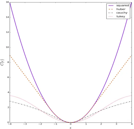
2.4.8 Robust Bundle Adjustment . . . 32
2.5 State Estimation . . . 33
2.5.1 Extension to non-linear systems . . . 36
2.6 MAV Control . . . 38
2.6.1 Quadcopter System Model . . . 38
2.6.2 Feedback Control . . . 41
2.6.3 Quadrotor Angular Velocity Control using PID . . . 43
2.6.4 Cascaded PID Control . . . 44
2.7 Conclusion . . . 46
3 Autonomous Navigation for Micro Aerial Vehicles 47 3.1 Absolute Positioning Approaches . . . 47
3.1.1 Radio Based Navigation . . . 47
3.1.2 Motion Capture Based Navigation . . . 49
3.2 Simultaneous Localisation and Mapping . . . 50
3.2.1 Laser Based Navigation . . . 50
3.2.2 Stereo Camera Based Navigation . . . 51
3.2.3 Single Camera Based Navigation . . . 52
Visual Markers . . . 52
Visual Odometry . . . 53
Visual Simultaneous Localisation and Mapping (V-SLAM) . . . . 56
The PTAM Algorithm . . . 57
Building on Keyframe-based Visual SLAM . . . 58
Direct methods . . . 60
Visual SLAM for MAVs . . . 61
Multi Robot Visual SLAM . . . 62
3.3 Summary . . . 65
4 Multi-robot Coordination Case Studies 67 4.1 Introduction . . . 67
4.2 Aerial Collision Avoidance Case Study . . . 67
4.2.1 Velocity Obstacles . . . 68
4.2.2 Reciprocal Velocity Obstacles (RVO) . . . 70
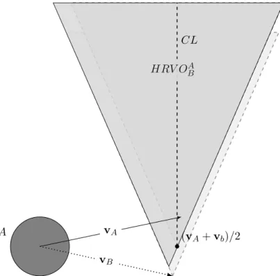
4.2.3 Hybrid Reciprocal Velocity Obstacles (HRVO) . . . 72
4.2.4 3D Velocity Obstacles . . . 73
4.2.5 The General Approach . . . 74
4.2.6 Evaluation . . . 77
4.3 Cooperative Exploration Case Study . . . 79
4.3.1 Interest Point Extraction . . . 80
4.3.2 Auction Mechanism . . . 81
4.3.3 Evaluation . . . 83
4.4 Conclusion . . . 83
5 A centralised approach to multi-robot Visual SLAM 85 5.1 Introduction . . . 85
5.4 CCTAM . . . 89
5.4.1 The Map . . . 89
5.4.2 Tracking . . . 89
5.4.3 Mapping . . . 92
5.5 State Estimation . . . 93
5.5.1 Sensor Observation Model . . . 94
5.5.2 Vision Observation Model . . . 94
5.5.3 State Transition Function . . . 95
5.6 Trajectory Control . . . 96
MAV Radius Scaling . . . 97
5.7 Implementation . . . 97
5.8 Evaluation . . . 98
5.8.1 Simulation Environment . . . 98
5.8.2 CCTAM Hardware Platform . . . 100
5.8.3 Localisation Performance . . . 100
5.8.4 Drift Analysis . . . 103
5.8.5 Scalability . . . 105
5.8.6 Multi-Robot Task 1: Collision Avoidance . . . 105
Real World Collision Avoidance Experiments . . . 106
5.8.7 Multi-Robot Task 2: Exploration . . . 107
5.9 Conclusion . . . 109
6 Distributed Collaborative Tracking and Mapping 111 6.1 Introduction . . . 111
6.2 Partially Distributed Visual Navigation . . . 112
6.3 System Overview . . . 113 6.3.1 The Map . . . 113 6.3.2 Tracking . . . 115 6.3.3 Stereo Initialisation . . . 116 6.3.4 Mapping . . . 117 6.4 Message Handlers . . . 119
6.4.1 Automated Stereo Initialisation Methods . . . 122
6.5 Additional Components . . . 123
6.5.1 Extended Kalman Filter (EKF) . . . 123
6.5.2 Trajectory Control . . . 123
6.6 Implementation . . . 124
6.7 DCTAM Hardware Platforms . . . 125
6.8 Evaluation . . . 127
6.8.1 Simulation Environment . . . 127
6.8.2 DCTAM Hardware Platforms . . . 127
6.8.3 Robustness . . . 128
6.8.4 Scalability . . . 128
6.8.5 Hardware Scalability Experiments . . . 133
6.8.6 Multi-Robot Task 1: Collision Avoidance . . . 135
Collision Avoidance Hardware Experiments . . . 136 v
6.8.9 Localisation Performance Hardware . . . 140 6.8.10 Tracking Performance on Hardware . . . 141 6.9 Conclusion . . . 144
7 Conclusions and Future Work 145
7.1 Publications . . . 150
A Open Source Hardware and Software 151
A.1 DCTAM Hardware and Software . . . 151
Bibliography 155
1.1 Small UAS: The SenseFly eBee (left) and Project Wing by Google (right) a VTOL craft delivering a package in the Australian outback. Image credits
to Sensefly and Google respectively. . . 1
1.2 Various MAV platforms: The Crazyflie Nano [22], a 20 gram MAV platform (left); the Flyabillity Gimball [27], a coaxial rotor driven platform surrounded by a gimbal mounted protective cage for enhanced collision protection (mid-dle); and the Honeywell RQ-16 T-Hawk [81], a ducted fan Vertical Take-off and Landing (VTOL) MAV developed by the United States military (right). 2 1.3 The general high-level system architecture for an autonomous MAV [119] . . 5
1.4 The MAV platforms used for the work presented in this thesis, the standard Parrot AR Drone (left) and a custom 3D printed, MAV platform (right). . . 6
2.1 MAV Coordinate Frames. . . 11
2.2 An illustration of the pinhole camera model. In reality the image plane is behind the camera centre and the true projection results in an image that is upside down and has to be rotated, this is done by the camera sensor so the generate images appear right way up. . . 13
2.3 An example of the lens distortion resulting for a wide angle lens(left) and the same scene after camera calibration and image rectification(right). . . 14
2.4 The segment test used in the FAST corner detector, here r= 3 and n= 12. The dashed arc highlights the 12 pixels brighter thanpthereforepis a corner feature [97]. . . 15
2.5 FAST corner features extracted from the image (left) and the corner features after non-maximum suppression(right). . . 18
2.6 FAST corner features extracted from an image (left) and corners with a Shi-Tomasi score> 50 (right). . . 18
2.7 Image Pyramid . . . 20
2.8 Perspective n-Point Problem . . . 21
2.9 Triangulation . . . 23
2.10 An example of a fiducial marker . . . 23
2.11 Epipolar Geometry . . . 24
2.12 Re-Projection Error . . . 26
2.13 Bundle Adjustment Problem . . . 28
to rotate at a certain speed. Each rotating propeller accelerates the air and induces a perpendicular forceFicounteracting the forceFgrav that pulls the
quadcopter towards the earth. . . 38
2.16 Quadcopter control: this diagram shows how varying the speeds of each motor results in a corresponding movement, red arrows indicate increased speed. Note the coupled rotational and translations movements on the pitch and roll axes. . . 40
2.17 Block diagram of a typical feedback control problem . . . 42
2.18 Block diagram of a Proportional Integral Derivative (PID) controller . . . 43
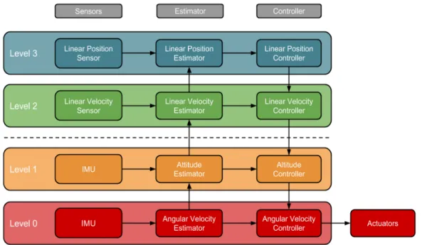
2.19 The general high-level system architecture for an autonomous MAV. . . 45
3.1 The two main sources of GPS interference, atmospheric (left) and multipath (right) [19]. . . 48
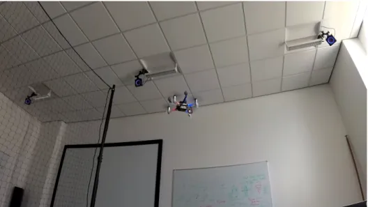
3.2 An example of using motion capture to control a palm sized Crazyflie Nano MAV in the University of Liverpool’s smARTLab. . . 50
3.3 The visual odometry problem, computing the motion of a camera from in-cremental computations of the relative transformation between images. . . . 54
3.4 Challenges of visual odometry on MAVs (right) the effect of height on mea-sured velocity and (left) the effect of rotation on meamea-sured velocity.[17] . . . 55
3.5 The original PTAM showing the real-time tracking of features in a typical office desk scene (left) and the corresponding map points (right). . . 58
3.6 A simple example of a loop closure situation. In the figure the robots tra-jectory is show as a solid line and it’s own tratra-jectory estimate is given as a dashed line. . . 59
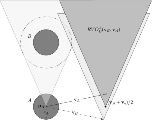
4.1 An example of Velocity Obstacles, here the VO of robot B with respect to robotA in absolute velocity space is illustrated by the dark gray cone. . . 68
4.2 Illustration of the oscillations that can occur when using the Velocity Ob-stacle approach [115]. . . 70
4.3 Illustration of the Reciprocal Velocity Obstacle (RVO) for the example in-troduced in Figure 4.1. . . 70
4.4 Illustration of how the RVO approach helps avoid oscillations that occur in situations similar to Figure 4.2. . . 71
4.5 Two examples of situations where robot A is unable to select a velocity outside the RVO. In the first example (left) RobotA’s goal location is given by G, the vector of the goal location meansA is unable to select a velocity outside the RVO induced by robot B. In the second example (right) the presence of a third robot C also restricts the choice of safe velocities for robotA. [105]. . . 72
4.7 An example of a crash resulting when a MAV attempts to avoid collision by passing over the other MAV. In the first image (left) the MAVs begin to pass over one another, in the second image (middle) the MAV is pushed down by the propeller wash of the MAV above, in the final image (right) the MAV
cannot maintain stable flight and hits the ground. . . 73
4.8 Controller architecture. . . 74
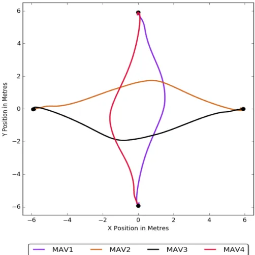
4.9 MAV trajectory plot for a collision avoidance experiment with 4 MAVs, the start location for each MAV is marked with a dot. . . 77
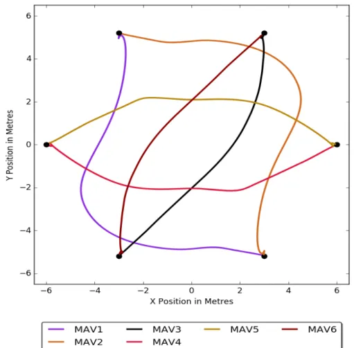
4.10 MAV trajectory plot for a collision avoidance experiment with 6 MAVs, the start location for each MAV is marked with a dot. . . 78
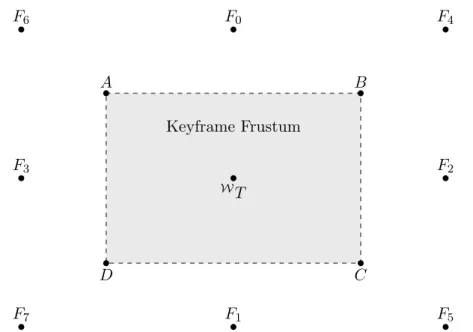
4.11 Illustration of the frustum based and candidate keyframe poses. . . 81
4.12 An example of frontier point extraction; the keyframe positions are shown as red arrows, the keyframe frustums are shown a blue rectangles and the frontier points as green dots. . . 82
5.1 The Parrot AR.Drone, a commercially available MAV platform used for the work presented in this Chapter. . . 86
5.2 An example of the blurred image re-localisation technique used in PTAM. . . 87
5.3 A high level overview of the CCTAM Framework. The main components are the MAVS which provided sensor data images to CCTAM which computes state estimates for the MAVs based on this data. This is passed to the position controller which compute suitable control commands to send to the MAVs. . . 88
5.4 The processes for a single MAV in the CCTAM system. . . 89
5.5 The CCTAM tracking process . . . 90
5.6 The CCTAM mapping process . . . 92
5.7 The simple simulation world . . . 98
5.8 The simulated disaster world . . . 99
5.9 A representative example of the CTAM localisation experiments. The dashed green line represents the ground truth trajectory and the solid coloured lines represent the trajectory for each MAV. . . 101
5.10 The result of the hardware localisation experiment, the ground truth trajec-tory is shown as a dashed green line and the esitmated trajectrajec-tory as a solid purple line. The RMSE for this experiment was 0.10 metres. . . 102
5.11 An example of localisation performance along a long trajectory. The trajec-tory length was 66 metres and the total accumulated drift was 0.66 metres. . 103
5.12 An example of localisation performance along a long trajectory with short loop closures. The trajectory length was 64 metres and the total accumulated drift was 0.05 metres. . . 104
5.14 MAV trajectory plot for a collision avoidance experiment with 3 MAVs, the start location for each MAV is marked with a dot and the end location a square. . . 106 5.15 Conducting collision avoidance experiments with real hardware . . . 107 5.16 An example the ground truth model of the simulated environment (top)
and the map-points produced by CCTAM (bottom). A comparison of these two pointclouds is used to determine the accuracy of the map produced by CCTAM. . . 108 6.1 Basic system overview of the DCTAM system. . . 113 6.2 An overview of the DCTAM Map data structure. The Map consists of a set
of keyframes and map-points, each keyframe contains a set of point mea-surements which reference a specific map-point. Each map-point contains a reference to the source keyframe from which the map-point was created. . . 114 6.3 The structure of the New KeyFrame message in DCTAM. The message
con-sists of a single keyframe as well as a set of measurement of existing map-points used when performing Bundle Adjustment. . . 116 6.4 Structure of the Stereo Initialisation message used by the DCTAM system. . 117 6.5 Structure of the Map Update message used by the DCTAM system. . . 117 6.6 Structure of the Bundle Adustment Update message used by the DCTAM
system. . . 118 6.7 The first DCTAM hardware platform based on the AR.Drone frame and PX4
flight controller. . . 124 6.8 The second DCTAM hardware platform based on a custom designed 3D
printed frame. . . 125 6.9 The dual processor architecture of the DCTAM hardware platforms. . . 126 6.10 Results of the delay experiment showing a delay of 600 ms (top) and 1000
ms (bottom). . . 129 6.11 Results of the bandwidth experiment showing the bandwidth requirements
for a single drone when operating alone (top) and as part of a team (bottom). Note how the requirement to transmit the keyframes to all MAVs increases the received messages whereas the sent messages remain the same. . . 130 6.12 Results of the scalability experiments, these graphs show the trjacectories
in 2D (top) and 3D (bottom) of 8 MAVs simultaneously exploring the same environment. . . 131 6.13 Results of the scalability experiments, these graphs show the trjacectories in
2D (top) and 3D (bottom) of 20 MAVs simultaneously exploring the same environment. . . 132 6.14 This graph plots the bandwidth requirements for a team of 20 MAVs. . . 134
6.16 Results of the repeated experiment featuring 20 MAVs, with the Trackers
running on real hardware, the final RMS error was 0.08. . . 135
6.17 A representative example of the simulated collision avoidance experiments. The start position of each trajectory is indicated by a circle marker and the end position a square. . . 136
6.18 A representative example of the hardware collision avoidance experiments. The start poisition of each trajectory is indicated by a circle marker and the end position a square. . . 137
6.19 An example the ground truth model of the simulated environment (top) and the map-points produced by DCTAM (bottom). A comparison of these two pointclouds is used to determine the accuracy of the map produced by DCTAM. . . 138
6.20 The figure show the performance of the new bundle adjustment implementa-tion with respect to reducing accumulated drift. The trajectory length was 63 metres and the total accumulated drift was 0.34 metres. . . 139
6.21 The figure show the performance of the new bundle adjustment implementa-tion with respect to reducing accumulated drift. The trajectory length was 74 metres and the total accumulated drift was 0.33 metres. . . 140
6.22 Results of a physical experiment with a single MAV navigating in a 2mx2m area; the RMS Error for this trajectory was 0.11 metres. . . 141
6.23 I7 desktop tracking time. . . 142
6.24 Odroid U3 tracking time. . . 142
6.25 Raspberry Pi3 tracking time. . . 142
6.26 Intel Atom tracking time. . . 143
6.27 This figure shows the average computation time for the tracking threads on a number of processors. . . 143
A.1 The AscTec Firefly MAV platform [110]. . . 151
A.2 A rendering of the 3D CAD model for the DCTAM hardware platform. . . . 152
A.3 The constructed DCTAM platform. . . 153
2.1 Motor mixing table for quadrotor, based on the motor order from Figure 2.15 44
4.1 Collision Avoidance Experiment Summary . . . 78
5.1 Localisation Performance Experiment Summary . . . 102
5.2 Collision Avoidance Experiment Summary . . . 106
5.3 Exploration Experiment Summary . . . 108
6.1 Collision Avoidance Experiment Summary . . . 136
6.2 Exploration Experiment Summary . . . 139
6.3 Bundle adjustment computations times on various map sizes . . . 140
6.4 Computer platforms used in the tracking performance experiments. . . 143
The following notations and abbreviations are found throughout this thesis: AGAST Adaptive Generic Accelerated Segment Test
BA Bundle Adjustment
BRIEF Binary Robust Independent Elementary Features CCTAM Centralised Collaborative Tracking and Mapping CPU Central Processing Unit
CSfM Collaborative Structure from Motion
DCTAM Distributed Collaborative Tracking and Mapping DOF Degrees of Freedom
DOG Difference of Gaussian
DTAM Dense Tracking and Mapping DWA Dynamic Window Approach EKF Extended Kalman Filter EoL End of Life
EPP Expanded Polypropylene
FAST Features from Accelerated Segment Test GPS Global Positioning System
GPU Graphics Processing Unit
HRVO Hybrid Reciprocal Velocity Obstacle ICP Iterative Closest Point
IMU Inertial Measurement Unit KLT Kanade-Lucas-Tomasi LM Levenberg-Marquardt
LSD-SLAM Large Scale Semi-Direct Simultaneous Localisation and Mapping MAV Micro Aerial Vehicle
MIMO Multiple Input Multiple Output ORB Oriented FAST and Rotated Brief P3P Perspective-Three-Point
PID Proportional Integral Derivative PnP Perspective n-Point
PTAM Parallel Tracking and Mapping PX4FMU PX4 Flight Management Unit
RGB-D Red Green Blue Depth RMSE Route Mean Squared Error RPY Roll, Pitch, Yaw
RVO Reciprocal Velocity Obstacle SAR Search and Rescue
SFM Structure from Motion
SIFT Scale Invariant Feature Transform SISO Single Input Single Output
SLAM Simultaneous Localisation and Mapping SSD Sum of Squared Differences
SSI Sequential Single Item
SVD Singular Value Decomposition SWaP Size Weight and Power
tf-idf term frequency-inverse document frequency UAS Unmanned Aerial Systems
UKF Unscented Kalman Filter VFH Vector Field Histogram VO Velocity Obstacles
ZSSD Zero-Mean Sum of Squared Differences
This thesis is primarily my own work. The sources of other materials are identified.
Micro Aerial Vehicles (MAVs), particularly multi-rotor MAVs have gained significant popularity in the autonomous robotics research field. The small size and agility of these aircraft makes them safe to use in contained environments. As such MAVs have numerous applications with respect to both the commercial and research fields, such as Search and Rescue (SaR), surveillance, inspection and aerial mapping. In order for an autonomous MAV to safely and reliably navigate within a given environment the control system must be able to determine the state of the aircraft at any given moment. The state consists of a number of extrinsic variables such as the position, velocity and attitude of the MAV. The most common approach for outdoor operations is the Global Positioning System (GPS). While GPS has been widely used for long range navigation in open environments, its performance degrades significantly in constrained environments and is unusable indoors. As a result state estimation for MAVs in such constrained environments is a popular and exciting research area. Many successful solutions have been developed using laser-range finder sensors. These sensors provide very accurate measurements at the cost of increased power and weight requirements.
Cameras offer an attractive alternative state estimation sensor; they offer high infor-mation content per image coupled with light weight and low power consumption. As a result much recent work has focused on state estimation on MAVs where a camera is the only exteroceptive sensor. Much of this recent work focuses on single MAVs, however it is the author’s belief that the full potential and benefits of the MAV platform can only be realised when teams of MAVs are able to cooperatively perform tasks such as SaR or mapping. Therefore the work presented in this thesis focuses on the problem of vision-based navigation for MAVs from a multi-robot perspective. Multi-robot visual navigation presents a number of challenges, as not only must the MAVs be able to es-timate their state from visual observations of the environment but they must also be able to share the information they gain about their environment with other members of the team in a meaningful fashion. The meaningful sharing of observations is achieved when the MAVs have a common frame of reference for both positioning and observa-tions. Such meaningful information sharing is key to achieving cooperative multi-robot navigation. In this thesis two main ideas are explored to address these issues. Firstly the idea of appearance based (re)-localisation is explored as a means of establishing a common reference frame for multiple MAVs. This approach allows a team of MAVs to very easily establish a common frame of reference prior to starting their mission. The
the structure and nature of the inter-robot communication with respect to visual navi-gation; the thesis explores how a partially distributed architecture can be used to vastly improve the scalability and robustness of a multi-MAV visual navigation framework.
A navigation framework would not be complete without a means of control. In the multi-robot setting the control problem is complicated by the need for inter-robot colli-sion avoidance. This thesis presents a MAV trajectory controller based on a combination of classical control theory and distributed Velocity Obstacle (VO) based collision avoid-ance. Once a means of control is established an autonomous multi-MAV team requires a mission. One such mission is the task of exploration; that is exploration of a previously unknown environment in order to produce a map and/or search for objects of interest. This thesis also addressed the problem of multi-robot exploration using only the sparse interest-point data collected from the visual navigation system. In a multi-MAV explo-ration scenario the problem of task allocation, assigning areas to each MAV to explore, can be a challenging one. An auction-based protocol is considered to address the task allocation problem. The two applications discussed, VO-based trajectory control and auction-based environment exploration, form two case studies which serve as the partial basis of the evaluation of the navigation solutions presented in this thesis.
In summary the visual navigation systems presented in this thesis allow MAVs to cooperatively perform task such as collision avoidance and environment exploration in a robust and efficient manner, with large teams of MAVs. The work presented is a step in the direction of fully autonomous teams of MAVs performing complex, dangerous and useful tasks in the real world.
The work presented in this thesis represents the completion of one of the biggest chal-lenges of my life to date. I would not have reached this point without the guidance, understanding and support from all the people who have been involved over the last few years. A lion’s share of that gratitude must go to my supervisory team Prof. Boris Konev and Prof. Frans Coenen. To Boris, I owe not only thanks for his insight and guidance throughout the years but also for giving me the opportunity to pursue a PhD in the first place. It has been a journey filled with many challenges, surprises, successes and failures but thanks to you it has been a fruitful one which I will cherish in the years to come. To Frans, I owe a lot for believing in me even when I had doubts, for always helping me stay on course and keep focus which has been invaluable while working to complete my thesis. I would also like to thank my advisers Prof. Wiebe van der Hoek, Prof. Michael Fisher and Dr. Muhammad Khan for their insightful questions and helpful comments that helped me see my work in a different light.
I would also like to thank Prof. Karl Tuyls for opening up new opportunities for me; both for your help in securing a teaching position and allowing me to participate in the Robocup and Rockin competitions. I will always be grateful to you for the invaluable lessons those experiences have taught me. To Prof. Simon Parson and Dr. Betsy Sklar, I owe thanks for their guidance and kindness in allowing me to use their lab space for my experiments. To my friend and colleague David Geleta I owe a special thanks, for being there for the whole epic journey from our Undergraduate days to the final days of our PhDs. You have been my Samwise and my Frodo, and I will forever be in your debt. To my fellow PhD students Eric Schneider, Jeffery Rafael, Gabrielle Dos Santos, Matoula Kotsialou, Bastian Broecker, Daniel Claes, Joscha Fossel and Dr. Daan Bloembergen who have been there for all the late nights, coffee breaks, wonderful celebrations, enjoyable and sometimes surreal University events, each of you have made these experiences all the more enjoyable by your involvement.
Finally and most importantly to my family. It is to my father, Michael that I owe thanks for sparking my love of technology. For putting up with my persistent, misguided attempts to electrocute myself which characterised many of my early attempts to emulate your mastery of all things electronic. For your patience and guidance throughout the years and for always being there when I had a difficult problem to solve. It is to my my mother I owe thanks instilling in me the courage, determinations and stubbornness
Introduction
1.1
Micro Aerial Vehicles
For several decades research into Unmanned Aerial Systems (UAS) has been dominated by the military and aerospace industries. The barrier for entry into these fields being the ability to deploy and support a large unmanned aircraft. However with advances in sensor and battery technologies, powered largely by the mobile phone market, it has become possible to develop smaller UAS. These small UAS come in a variety of configurations from fixed-wing aircraft (Figure 1.1 (left)) capable of long duration, high altitude flight, to highly stable and manoeuvrable rotary-wing craft such as helicopters and quad, hexa and octocopters. More recently several hybrid Vertical Take-Off and Landing (VTOL) systems have been developed capable of transitioning between hovering and fast forward flight (Figure 1.1 (right)).
The number of civilian and humanitarian applications of these craft has also been growing, systems such as the SenseFly eBee (Figure 1.1 (left))see have been used in the aftermath of several natural disasters for rapid damage assessment and monitoring of temporary settlements [35]. Several companies including Google and Amazon have begun development of small UAS for tasks such delivering medical supplies to remote locations as well as commercial goods delivery in urban environments.
Figure 1.1: Small UAS: The SenseFly eBee (left) and Project Wing by Google (right) a VTOL craft delivering a package in the Australian outback. Image credits to Sensefly
and Google respectively.
Micro Aerial Vehicles (MAVs) are a class of small UAS typically with limitations on size and payload. The term MAV is sufficiently ambiguous to have been used to describe craft weighing from 100 grams to several kilograms as shown in Figure 1.2. In the context of this thesis a MAV is defined as an aerial vehicle which weighs under 5 kilograms, is less than 1 metre in length and is capable of operating safely within a typical indoor environment such as office buildings. In this thesis the focus is on multi-rotor MAVs, specifically quadcopters; however the work presented is applicable to most rotary-wing aircraft and with some modifications could be applied to fixed wing aircraft as well.
Figure 1.2: Various MAV platforms: The Crazyflie Nano [22], a 20 gram MAV plat-form (left); the Flyabillity Gimball [27], a coaxial rotor driven platplat-form surrounded by a gimbal mounted protective cage for enhanced collision protection (middle); and the Honeywell RQ-16 T-Hawk [81], a ducted fan Vertical Take-off and Landing (VTOL)
MAV developed by the United States military (right).
There are numerous applications for MAVs such as: Search and Rescue (SaR), aerial inspection, exploration and conservation activities such as wildlife or crop monitoring [37]. These applications all have one thing in common, a requirement for a robust and reliable navigation system. The standard navigation solution for MAVs utilises the Global Positioning System (GPS) as the main localisation solution. However, GPS has several limitations in terms of both accuracy and coverage (more in Chapter 3) and there are many applications where GPS cannot be used, for example indoor SaR [80].
Given that SaR is an ideal application for MAVs their actual deployment in real SaR situations is surprisingly infrequent as noted by a recent study by Murphy et al. [80]. Murphy et al.s study covers all cases of robots being deployed in disasters between 2001 and 2013 and shows that of the 34 documented incidents there were only 10 incidences of MAVs being deployed. Additionally, Murphy et al. highlight the fact that while there have been cases where MAVs have had autonomous capabilities they were never used in any of these 10 cases. Murphy et al. give several reasons for the lack utilisation of autonomous capabilities, she notes that in several cases the craft were operating close enough to structures to cause interference to the crafts (GPS) based navigation systems. In general it comes down to a lack of trust in the autonomous systems; the pilots did not feel comfortable in delegating control to an autonomous navigation system even in cases where the autonomous system was more than capable of achieving the current objectives. This is evidenced by the fact that while there is increasing use of MAVs in real world
applications these tend to be either manually controlled or in highly structured settings where lack of advanced capabilities such as collision avoidance and scene perception are not required.
One major difficultly in multi-rotor research is the significant investment of both time and capital required to set-up a safe, reliable framework with which to conduct research. Some of the most common MAV research platforms are the AscTec1 line of multi-rotor MAVs. These platforms typically cost in the range of e5000-8000. These platforms are also by no means complete solutions as additional sensors and on-board computers are still required. This also does not include any localisation system; which, depending on the aims of the individual researchers, may not be an issue however it is argued here that, for safety reasons, some form of localisation system is required. This is mainly due to the highly dynamic nature of MAVs and the lack of robust emergency recovery. It’s common to include an emergency stop button on a ground robot which will immediately cut-off power to the actuators in the case of a runaway robot. However this is not possible with MAVs; indeed immediately cutting power to the actuators on a multi-rotor MAV virtually guarantees significant damage to the craft. However with the inclusion of a localisation system the safety of the craft immediately improves. They allow the MAV to perform controlled emergency landings or restrict their movements to only a specified area (this is often called fencing). The specifics of multi-rotor localisation systems will be discussed in Chapter 3. However, given the above the barrier for entry into the field of practical MAV research in general, and multi-MAV research in particular, is very high from both a monetary and safety standpoint. This has been noted by other researchers as a recent survey by Farid Kendoul of unmanned rotor-craft systems (a general term used to refer to both small and large rotary wing craft) [51]. Kendoul noted that while significant theoretical work has gone into autonomous navigation of UAS there is a gap between the theoretical work and the practical experimentation done. This thesis proposes that the barrier for entry, as discussed above has influenced development of this gap. By focusing on the development of solutions for low-cost, computationally constrained platforms the intention is to not only address a challenging research topic, but also help close the gap between theory and experiment and encourage more researchers to conduct practical experiments.
1.2
Autonomous Navigation for MAVs
In this Section the problem of autonomous navigation is introduced and discussed in the context of MAVs. The autonomous navigation problem is typically divided into three main challenges:
• Localisation: Where are the MAVs relative to their environment and each other?
• Mapping: What does the environment look like?
1
• Navigation: What path must the MAV follow in order reach a target location? Also, given a path, what control commands are required to follow it?
The localisation problem entails determining the pose (position and orientation) of a robot with respect to its environment based purely on the processing of sensor data. A reliable means of achieving this to give the robot a model of the environment in the same, or similar format, as its sensor data. For example if a robot, equipped with a camera, is given a model of its environment consisting of visual features, then it can solve the localisation problem by comparing the features it sees to those in the model. Constructing a model by hand is not always easy, how does one construct a model of the visual features in a room by hand? One way to solve this problem is to make use of an existing means of localisation. Then a model of the environment can be constructed by incrementally fusing observations of the environment together. This is referred to as mapping the environment. This requires some existing, usually external, localisation system and a separate mapping phase before the system can be deployed to do anything useful. This is not ideal with respect to many applications. It would be ideal if the robots were to be able to localise in novel environments, this means being able to simultaneously localise within and construct a map of a previously unknown environment. This is commonly referred to as the Simultaneous Localisation and Mapping (SLAM) problem [5].
The navigation problem is also divided into two parts: path planning and trajectory execution. Path planning is the problem of determining the route from a robot’s current location to it’s goal location, typically in the shortest time possible while avoiding all obstacles. The output of the path planner is a trajectory to be executed by the robots control system; depending upon the type of robot platform the trajectory execution problem can have its own challenges and constraints. For example, on fixed-wing MAVs trajectory execution can be complicated by the fact that the craft must keep moving in order to stay in the air. The path planning and trajectory execution problems can also be tightly coupled with the SLAM problem, as whatever environment model used for mapping and localisation is typically used for path planning. The reliability of the localisation method also has a big impact on the trajectory execution. For example a visual localisation approach may be affected by motion-blur; therefore, during trajectory execution, the MAV should avoid rapid accelerations as these may result in localisation failure. The typical high-level architecture of a robot navigation system is show in Figure 1.3. As the work in this thesis aims to explore the navigation problem from a multi-robot perspective “Other MAVs” have been included in the diagram to highlight those components in the navigation system that are affected by the inclusion of other robots into the system. The multi-robot navigation problem is explained in more detail in the next section.
Figure 1.3: The general high-level system architecture for an autonomous MAV [119]
1.3
Multi-robot Navigation and Coordination
In this thesis the focus is the problem of multi-robot visual navigation on MAVs and how this relates to the problem of multi-robot coordination for tasks which are tightly coordinated. There is much work, particularly in the field of swarm robotics, which investigates loosely-coordinated solutions in which individual robots have either limited or no awareness of the explicit goals and behaviours of other robots, interaction is limited and coordination is emergent rather than strictly defined. The work presented in this thesis is concerned with direct coordination between multiple robots for tightly coupled tasks which require significant interaction and coordinated execution. This places additional constraints on the navigation system as not only must the robots be able to localise themselves (while mapping) but they must be able to localise themselves within a common coordinate system.
This becomes apparent when a simple search and rescue scenario is considered: two MAVs are tasked with searching a building to find a person in need of medical attention. MAV1 is smaller and faster so is tasked with exploring the building to find the person. MAV2 is larger and can carry a heavier payload and is tasked with both exploring the building and bringing the medical supplies. Both MAVs have no map of the building so are required to build one as they go. MAV1 explores the building and eventually finds the person and communicates to MAV2 the location of the person according its own map. However MAV2 is unable comply as the communicated coordinates are in MAV1s map frame which is unknown to MAV2. Even if MAV1 were to share its map with
MAV2 there is no guarantee this would result in success as it requires MAV2 to combine the two maps which is only possible if there is a common point of reference. In this thesis two multi-robot coordination problems are explored and use is made of them as case studies to verify the performance of the proposed visual navigation approaches. The first is a market-based approach to environment exploration. This tackles the problem of environment exploration using an auction-based protocol to assign exploration goals to individual MAVs. Another essential coordination task when dealing with groups of aerial vehicles in close proximity is that of MAV-to-MAV collision avoidance. A multi-robot distributed approach to collision avoidance based on velocity obstacles is also explored.
Figure 1.4: The MAV platforms used for the work presented in this thesis, the stan-dard Parrot AR Drone (left) and a custom 3D printed, MAV platform (right).
1.4
Research Questions and Contributions
Multi-robot Visual Navigation is a complex problem. In this thesis the problem is explored from the standpoint of two important requirements, those of scalability and robustness. The goal is to develop a robust, scalable multi-robot visual navigation system capable of being deployed using low cost MAVs (see Figure 1.4). The research goals that the work presented in this thesis seek to address are summarised by the following research questions:
1. How can a Visual SLAM and appearance based localisation be used to support the autonomous navigation of large teams of low cost Micro Aerial Vehicles? 2. Given the above how does the architecture of the proposed navigation system affect
its scalability and robustness?
3. The barrier for entry for practical research using multiple MAV systems is still high due to the cost of the most commonly used external localisation systems. Can this be addressed by the introduction of alternate approaches based on visual SLAM and low cost platforms?
4. Can a visual SLAM based navigation approach be used to support more high level research such as multi-agent coordination?
In the context of the above research questions the following is a summary of the key contributions of the work presented in this thesis.
1. An examination of the concept of using place recognition to enable multi-robot visual navigation for teams of MAVs which is presented in Chapter 4. This work explores this idea with a proof-of-concept implementation of a centralised multi-robot visual navigation system for the Parrot AR. Drone. The approach is based on Parallel Tracking and Mapping (PTAM) [54], a ground-breaking visual SLAM approach developed by Klien and Murray. This facilitates the use of an extremely low cost (<£300) and light weight (<500 grams) MAV platform for multi-robot research.
2. A general, scalable, partially distributed tracking and mapping system for teams of MAVs which is presented in Chapter 5. Here our previous fully centralised ap-proach is built upon to achieve a more robust, highly scalable, distributed visual navigation system. A more general state estimation approach together with alter-nate stereo initialisation methods make the distributed approach applicable to a range of MAV platforms.
3. Experiments to analyse the performance of both the centralised and distributed approaches in terms of localisation performance, scalability and robustness which are presented in both Chapters 4 and 5. It is shown that both approaches exhibit on average a Route Mean Squared Error (RMSE) of less than 10 centimetres and it is demonstrated that the centralised approach is capable of scaling to teams of up to 4 MAVs. In contrast experimental results are presented which show the distributed approach is capable of scaling up to 20 MAVs. Finally the increased robustness to network delay afforded by the distributed approach is demonstrated. This increased robustness is shown to improve the reliability of real-time motion tracking and localisation.
4. A demonstration of how the precision and reliability of the proposed visual navi-gation approach, in combination with a reciprocal velocity obstacle based position controller, can be used to solve the difficult problem of mid-air collision avoidance. This work is presented in Chapter 6.
5. An application utilising the sparse feature-based map produced by our visual navi-gation system to implement an auction-based multi-robot environment exploration system. This work is presented in Chapter 6.
6. Open source implementations of all software and hardware developed for this thesis aimed at lowering the bar for entry into this line of research. It is the author’s hope that the available of the software developed in this thesis will encourage more researchers to conduct real physical experiments using MAV platforms and help bridge the knowledge gap discussed previously. This is discussed in Appendix A.
1.5
Thesis Outline
The remainder of this thesis is organised as follows. Chapter 2 introduces preliminaries including the notation used as well as the theoretical background of the camera model, feature detection, structure from motion, state estimation and control. Chapter 3 looks at state of the art solutions to MAV navigation and motivates the use of vision as the primary navigation sensor. Further common visual localisation methods, for both single MAV as well as teams of MAVs are reviewed. While the main focus of this thesis is visual navigation two multi-robot coordination case studies: robot-to-robot collision avoidance and multi-robot environment exploration are also considered in Chapter 4. The ideas and algorithms developed to address these case studies are discussed as well as their applicability in the evaluation of the visual navigation approaches developed for this thesis.
In Chapter 5 the idea of appearance based localisation to enable multi-robot visual navigation is explored; a proof of concept implementation is developed which forms the basis of one of the contribution of this thesis namely a centralised multi-robot visual navigation system. A complete quantitative evaluation of the framework is also presented including localisation, mapping and scalability experiments. In addition the framework performance in two multi-robot coordination tasks (collision avoidance and exploration) is evaluated.
In Chapter 6 the idea of a partially distributed approach to multi-robot visual navi-gation is explored. The chapter explores the benefits in terms of performance, robustness and scalability compared to the centralised approach. A platform agnostic implemen-tation of this distributed visual navigation approach is also presented. Chapter 5 also presents an evaluation of the new distributed approach in terms of localisation accuracy, robustness to delay and bandwidth requirements. The distributed approach is also put to the test in the two multi-robot coordination tasks (collision avoidance and explo-ration). Finally Chapter 7 concludes the thesis with an overall analysis of the research as well as a discussion of future work.
Preliminaries
In this chapter the foundational concepts of geometry, computer vision and Simulta-neous Localisation and Mapping (SLAM) used throughout this thesis are introduced. In Section 2.1 we start by fixing the notation for geometric primitives and describe a number of relevant transformations. Section 2.2 explores how we represent images, in particular we look at perspective projection and the pinhole camera model. In section 2.3 we look a extracting interest points from images and how they may be used to solve problems such as image stitching and camera tracking. Section 2.4 covers theory and algorithms for deriving 3-dimensional (3D) structure from 2-dimensional (2D) images often referred to as photogrammetry or Structure from Motion (SfM). We conclude the chapter in Sections 2.5 and 2.6 by looking at two related problems in robotics: state estimation using Kalman filters and feedback control. The material in this Chapter in based on the excellent book by Szeliski [109] (in particular Chapters 2, 4 and 7).
2.1
Points and Vectors
In this section we fix the notation and briefly describe the geometric primitives used in this work. Starting with points, we represent a point in terms of either: (i)n-dimensional Cartesian coordinates or (ii) n+ 1 homogeneous coordinates where points differing by only their scale factor are equivalent:
X= x y z ˜ X= x y z w Where x y z = x/w y/w z/w 9
To improve clarity we distinguish between a 2D and 3D point/vector with capitalisation. For example a 2D pointxin homogeneous coordinates or a 3D pointX in homogeneous coordinates: ˜ x= x y w ˜ X= x y z w
2.1.1 Rigid Body Transformation
Points and vectors are typically represented with respect to a designated coordinate frame. Where relevant we will denote the coordinate system of a point by a leading superscript, for example the 3D point X in the world coordinate frameW will be rep-resented asWX. Rotations can be expressed most generally by a 3×3 rotation matrix in the rotation group: R∈SO(3).
R= r11 r12 r13 r21 r22 r23 r31 r32 r33
This representation has some nice properties:
R−1 =RTdet(R) = 1
The rigid body, or 3D Euclidean transformation is one which translates point(s) from one coordinate system to another and is described by a transformation matrix of the form: WCH˜ = " R t 0T 1 # = r11 r12 r13 tx r21 r22 r23 ty r31 r32 r33 tz 0 0 0 1
Where: (i)WCH˜ denotes the transformation from the world coordinate frame W to the camera coordinate frame C, (ii) R is the 3×3 rotation matrix and (iii) t is a 3×1 translation vector. The rigid body transform is used throughout the work in this these to describe the pose (position and orientation) of a MAV with respect to a global coordinate system as well as for transformations between coordinate frames. The rigid body transformation WCH˜ is a member of the Lie group SE(3), which allow the rigid body transformation to be minimally parametrised by a six dimensional vector µ via the exponential map. This representation has many desirable properties including being trivially differentiable. Full details of the Lie group SE(3) and its applications can be found in [116].
IN IE ID TIB BX BY BZ
Figure 2.1: MAV Coordinate Frames.
Figure 2.1 shows the common coordinate frames for a MAV as used in this thesis. The inertial frame I is the earth fixed coordinate system with the origin defined as the starting or home location. Thex-axis points north, they-axis points east and thez-axis points into the earth. The coordinate system of a MAV is described by the body frame
B, where the origin is located at the centre of mass of the MAV. The x-axis points towards the front of the MAV, the y-axis points to the right of the MAV and the z
axis points downward from the MAV. The transformation from the inertial frame to the body frame is given by the rigid body transformIBT˜.
In some reported work, particularly that relating to MAV control, additional frames are introduced which separate the rotation and translation components of the transform
IBT˜. For example a vehicle frame V can be introduced where the origin is located at
the centre of mass of the MAV but each axis is aligned with the inertial frame. This means the translation of the MAV with respect to the inertial frame can be expressed by the transformIVT˜ and the rotational component of the transform can be expressed as a pure rotation from the vehicle frame to the body frame VBR.
2.1.2 Similarity and Affine Transformations
TheSimilarityorScaling Transformis part of the group containing similarity trans-forms in three dimensional space Sim(3). It has the same representation as the rigid
body transformation with the addition of a scale factor: ˜ X0= " sR t 0T 1 # ˜ X
The addition of the scaling factor to the similarity transform is useful, particularly for monocular SLAM where the scale is unknown or estimated using data from metric sensors. Optimisations such as loop closures, pose graph optimisation and bundle ad-justment (see Section 2.4.5 can be done using the similarity transform instead of the standard rigid body transform. This allows us to take the scale ambiguity into account during optimisation [107].
The Affine Transformation goes a step further by adding a shearing factor along each axis: ˜x0=A˜xwhere: A= a11 a12 a13 a21 a22 a23 0 0 1
The affine transformation is useful to describe the transformation of points between images. In such cases, where image features are observed from different viewpoints, the rigid body or similarity transform is not sufficient to describe the transformation of the points.
2.2
Pinhole Camera Model
This Section focuses the foundational concepts of computer vision used for the work presented in this and how they relate to the problem of visual navigation. In partic-ular this Section will cover how visual observations using cameras are modelled using the pinhole camera and distortion models. The section concludes with a discussion of geometric image features and feature matching.
The pinhole camera model describes the projection of 3D world features into the image plane of an ideal pinhole camera. It is used throughout computer vision to model the transformation from the 3D world of objects to the 2D world of images. This model illustrated in Figure 2.2 where the 3D world point P˜ is projected onto the image plane of the camera at image point ˜x. The pinhole camera model is an example of the most general type of transformation, perspective projection. Given a 3D point in the world observed by a camera we often want to compute its corresponding 2D point in the image plane. The pinhole camera model can be described in matrix form by:
x y w = fx s cx 0 fy cy 0 0 1 X/Z Y /Z 1
Where: fx and fy define the focal length of the camera (in pixels) (this representation
• Z Y X • ˜ x •P˜ • x y camera centre image plane
Figure 2.2: An illustration of the pinhole camera model. In reality the image plane is behind the camera centre and the true projection results in an image that is upside down and has to be rotated, this is done by the camera sensor so the generate images
appear right way up.
centre (also called the principal point) and sdefines the skew factor to account for the sensor not being mounted perpendicular to the optical axis [109]. The skew factor is often omitted as most image sensors do not induce any axis skew. These parameters can be provided by the manufacturer or more commonly obtained via calibration (see Section 2.4.1). This model assumes the 3D coordinates describe the point relative to the camera centre. If coordinates describe the transform relative to some other coordinate system e.g. WP˜ in the world frame W the point must first be transformed to the camera coordinate system. This means we must know the camera transform in the world coordinate system, this is generally described as the extrinsic parameters of the camera:
Mext=
h
WCR Cti
Thus a 3×4 matrix describing the WCRworld to camera rotation whereCt is the world origin in camera coordinates. Therefore the full camera matrix containing both the intrinsic and extrinsic parameters of the camera is required to translate a point from world coordinates to (u, v) pixel coordinates:
˜ x=KMextWP˜ (2.1) x y w = fx s cx 0 fy cy 0 0 1 r11 r12 r13 tx r21 r22 r23 ty r31 r32 r33 tz X Y Z 1 (2.2)
" u v # = " x/w y/w # (2.3) 2.2.1 Lens Distortion
The model above assumes no distortion occurs i.e. a perfectly shaped lens. However in practice this is not the case and imperfect lenses and sensor alignment can introduce significant distortion. This distortion results in image points appearing in significantly different positions than the expected projection given by the pinhole camera model de-scribed in the previous section. This is particularly noticeable when observing lines, straight lines in the world appear curved in the image. This effect is even more pro-nounced with wider angle lenses as shown in Figure 2.3. A common approach is to use a low order polynomial to model the radial distortion:
xcorrected =x(1 +k1r2+k2r4+k3r6) (2.4)
ycorrected =x(1 +k1r2+k2r4+k3r6) (2.5) Where r2 = x2+y2 accounts for the increasing distortion the further from the centre point and k1, k2 and k3 are the radial distortion coefficients estimated via calibration. For wider angle lenses such as those used in this thesis it is more efficient to model the distortion using Devernay and Faugeras’ Field of View (FOV) model[18]. In the FOV
Figure 2.3: An example of the lens distortion resulting for a wide angle lens(left) and the same scene after camera calibration and image rectification(right).
model only a single parameter is used to describe the field of view of theidealwide-angle lens. It is assumed that the distance between an image point and the principal point is proportional to the angle between the corresponding ray connecting the 3D point with the optical centre and the optical axis in the rectified image. The radial distortion function is given as:
r=
r
x2+y2
r0 = 1
warctan(2r tan w
2) (2.7)
Wherew is the field of view parameter obtained via calibration. Recovering the undis-torted pixel coordinates can be done using the following transformation:
" x y # = r 0 r " x/w y/w # (2.8)
Some cameras also exhibit tangential distortion caused by misalignment between the lens and the image sensor, but it has been shown for the machine vision cameras used in this thesis that the effect is negligible [18].
2.3
Image Features
One of the fundamental problems in computer vision is feature detection and matching. Visual features are subsets of image data that describe unique or interesting regions within the image. Good features have desirable properties such as distinctiveness and repeatability. The ability to match unique features between two images allows a number of interesting applications such as image stitching, object tracking or, for the work in this thesis, case motion estimation. Features can describe geometric shapes such as lines and corners or less rigidly defined regions such as coloured/textured blobs. Corner points have been widely used in computer vision as interest points as they are highly constrained in both axes (as opposed to lines) and are therefore easier to match.
Figure 2.4: The segment test used in the FAST corner detector, here r = 3 and n= 12. The dashed arc highlights the 12 pixels brighter thanpthereforepis a corner
feature [97].
2.3.1 Corner Feature Detection
A feature detector is an algorithm which extracts visual features from images. A good feature detector is one that is both computationally efficient as well as reliable. For
real-time tracking applications such as visual SLAM, where feature extraction will be carried out on every image the importance of an efficient detector is vital. As such many tracking approaches use the Features from Accelerated Segment Test (FAST) detector. The FAST feature detector, first presented in [96], uses the Segment-Test algorithm to determine if there is a corner feature at some pixel locationp. The Segment Test is as follows, in a Bresenham [9] circle centred on pixel p and of radius r, if more than n
pixels are either brighter or darker than pixel p by some threshold t thenp is a corner feature see Figure 2.4. Adjusting the value oft determines the sensitivity of the corner detector, higher values oft results in a detector that finds fewer, but stronger, corners; a lower value increases the number of corners detected, but the resulting corners have smoother gradients which may affect repeatability.
The segment test can be accelerated as it provides a method to quickly reject pixels that definitely aren’t corner features. In the example in Figure 2.4 where n= 12, the pixels at each compass point (i.e. 1, 9, 5 and 13) can be checked first; if the intensity of these pixels is close to p then p cannot be a corner feature. This begs the question, whatever the value of n what is the fewest number of pixel intensity tests we can do to determine if p is a corner feature and what is the best value for n. The value of n
determines the maximum angle of the corner features detected while still rejecting edges (i.e. n= 8). Therefore n= 9 is the ideal value as it will detect corners with the largest variety of angles while still rejecting edges. In [97] Rosten demonstrated that a n= 9 detector is up to twice as fast as the original detector as well as being highly repeatable when compared to other state-of-the-art detectors.
The FAST-9 detector made use of machine learning to improve the performance of the segment test algorithm, for a given value ofnthe aim was to test the fewest number of pixels to determine ifp is a corner feature or not. Rosten used the full Segment Test to extract corner features to create a training set for a decision tree classifier. The aim being to produce a decision tree which can determine if a pixel contains a corner point by testing the fewest number of pixels. Rosten was able to produce an n= 9 detector which only needed to test an average of 2.83 pixels to determine if a corner feature is present. The reliance on supervised learning to build the decision tree means for the best results the FAST-9 detector should be trained on features collected from the operating environment. This reduces the adaptability of the detector, an issue addressed by Mair et al. with their Adaptive Generic Accelerated Segment Test (AGAST) detector [73]. The AGAST detector uses a more generic binary decision tree instead of the learned ternary tree used in FAST-9. It also combines two decision trees, one optimised for homogeneous or cluttered image regions and the other optimised for uniform surfaces or high structured regions with texture. The AGAST detector switches trees based on the local structure of the image, making it adaptable to different environments without training. This adaptability is particularly useful in the application of Visual SLAM in outdoor scenes as the environment can change from highly cluttered scene (e.g. buildings and infrastructure) to uniform, highly textured regions such as fields or roads.
2.3.2 Corner Feature Selection
A potential issue with feature detection is the problem of features detected adjacent to one another. This can lead to issues when matching features from other views in that the adjacent features could be erroneously matched given their proximity. A common solution is non-maximum suppression, where features adjacent to one another are filtered by their relative intensity. This is done by defining a scoring function for feature points,
V(p) whereV returns the sum of absolute difference betweenp and the 16 surrounding pixels. Scores of adjacent feature points are computed and the point with the lower score is discarded as illustrated in Figure 2.5. Another scoring function is the Shi Tomasi Scoring [103] function. This is based on the Harris Stevens [39] corner detector which uses the image gradients to detect corners. Specifically it computes a sum of squared difference matrixM over a small rectangular or Gaussian window functionw
M =X x,y w(x, y) " IxIx IxIy IxIy IyIy # (2.9)
Here Ix and Iy are the image gradients inx and y directions. This works well for
axis-aligned corner features; to obtain rotation invariance the corner response is computed using the Eigenvalues ofM:
M =R−1 " λ1 0 0 λ2 # R (2.10)
Where R is a matrix of the eigenvectors and λ1 and λ2 are the eigenvalues of M. The Harris Stevens detector computes the corner response function R with a tuneable sensitivity parameterk as
R=λ1λ2−k(λ1+λ2)
Indeed Harris and Stevens presented a method to approximate the corner response without explicitly calculating the Eigenvalues which are more computationally intensive.
R=detM −k(traceM)2
Where detM is the determinant of the matrix M and is equivalent to the expression
λ1λ2 andtraceM is the trace of matrix M which is equivalent toλ1+λ2. Shi and Tomasi noted that for reliable tracking, the features with the largest Eigenvalues that do not differ significantly are best [103]. These represent features with strong intensity profiles i.e. the intensity of the feature point differs to a larger extent than the mean intensity of the surrounding pixels. Given that the eigenvalues are bounded by the maximum intensity of the image it serves to take the smaller of the two to compute the corner score:
Whereλis a threshold parameter. An example is shown in Figure 2.6 where the image on the left shows the FAST corners detected in the image and the image on the right contains only those corners with a Shi Tomasi score above 50.
Figure 2.5: FAST corner features extracted from the image (left) and the corner features after non-maximum suppression(right).
Figure 2.6: FAST corner features extracted from an image (left) and corners with a Shi-Tomasi score> 50 (right).
2.3.3 Scale Invariant Feature Transform (SIFT)
Another interest point detector is SIFT[68]. SIFT is a combination of the Difference of Gaussian (DoG) feature detector and descriptor that uses gradient histograms. For the DoG detector the image is blurred using a Gaussian filter of increasingσ and computes the pairwise difference of the blurred images. Then for each pixel and a small window of neighbouring pixels it looks for the local extrema over all these Difference of Gaussian images, effectively searching for the scale at which the feature response is highest. The candidate points are filtered using non-maximum suppression, eliminating edges. Finally the precise centre point of the feature is computed at sub-pixel accuracy by fitting a quadratic function to the feature response function.
To achieve rotation invariance the dominant orientation(s) of the feature is computed using a histogram of local gradient directions. The highest peak and all peaks within a threshold of the highest peaks are selected. In the case of multiple peaks a feature point is generated for each dominant orientation. The feature descriptor is computed based on a 16×16 pixel region around the feature points. This is divided into 4×4 pixel regions on which an 8-bin orientation histogram is computed. This results in a descriptor with 128 elements. Their invariance properties make SIFT features a popular choice for applications such as image stitching and object recognition. For real-time tracking applications SIFT features are less popular due to the increased complexity involved in both SIFT feature detection and descriptor extraction. However in recent years, with the advances in parallel computation, using computer graphics processors it is possible to compute SIFT features in real-time [42].
2.3.4 Feature Matching
Feature detection is only one part of the problem in order to be useful we must be able to establish feature correspondences, that is, determine if featurex in imagei is the same 3D world point as featureyin image j. The local appearance of a feature in an image is subject to change in transformation, rotation, scale and illumination making this one of the most challenging problems in computer vision. Given the fundamental nature of the problem there are many solutions, a complete description of which, is beyond the scope of this work. The discussion will thus be restricted to discussing methods for matching the features discussed in this thesis namely FAST and SIFT. One particular method commonly used in conjunction with FAST features is template matching. Template matching involves a direct comparison of the intensity values of a small, fixed size, region of pixels around a detected feature point. It is based on the assumption that the intensity values of the templates remain consistent between frames. This assumption is valid in real-time tracking applications where the motion between frames in small. We can then compare image patches using the Sum of Squared Differences (SSD):
SSD = X
(u,v)∈W
(I1(u, v)−I2(x+u, y+v))2 (2.12)
Where an exact match of the intensity values will return a score of 0. A more robust but computationally more intensive approach is the Zero-Mean Sum of Squared Differences (ZSSD). Here the mean intensity value for each image patch is subtracted to improve robustness to lighting conditions:
ZSSD= X
(u,v)∈W
((I1(u, v)−I1)−(I2(x+u, y+v)−I2))2 (2.13)
Where I is the mean intensity of the pixel values in image patch I. This technique is often combined with an image pyramid to achieve a limited invariance to scale. An image pyramid is constructed by taking the source image applying a smoothing filter
Figure 2.7: Image Pyramid
and sub sampling it by some factorλalong each axis. This multi-scale representation of the image allows us to detect features at different scale levels providing some invariance to scale. The scaling factorλdetermines the number of pyramid levelsλ= 2 results in a 4 level image pyramid (see Figure 2.7). This patch-based approach has the advantage of being computationally efficient, however it relies on the consistency of intensity values between frames. Where there is a large difference in viewpoint the local intensity of matching templates may be vastly different.
Matching SIFT keypoints (and descriptors in general) is usually done using a nearest neighbour approach where the similarity measure is the Euclidean distance in feature space: d= [ 128 X i=1 (pi−qi)2]1/2
where pi and qi are the SIFT feature descriptors being compared. The naive approach
is to set an absolute threshold for the feature distance, however this can result in false matches. Instead Lowe et al. [68] suggested that the most robust approach was the threshold between the first and second nearest neighbours. If both are close (as defined by the threshold) then the pair cannot be described as a strong match and should be discarded. This means only the strongest matches are used. This can be done in a brute force manner with in complexity of O(m·n) to reduce a feature set of sizem to a set of size n. This makes real-time implementation infeasible but there are several approaches to reduce the complexity such as approximate nearest neighbour search [78] or the bag-of-words method [87].
YW ZW XW (R, t) c0• • x1 • x2 • x3 • p1 •p2 • p3
Figure 2.8: Perspective n-Point Problem
2.4
Structure from Motion
Recovering 3D information from a 2D camera sensor is a well known problem in computer vision, the key is exploiting either the motion of the object being observed or the motion of the camera itself to recover the missing depth information. Structure from Motion (SfM) has been extensively studied in the case of offline 3D reconstruction, however in recent years the techniques developed have been applied to real-time problems in robotics. In this section we will introduce some key problems in SfM and describe some common methods to solve them. In particular we will look at the problems of estimating the pose of a camera when observing a known shape, recovering depth information from two distinct views of the same point and estimating the relative pose between two cameras. We will conclude with a discussion of bundle adjustment, a powerful technique to iteratively refine both structure (3D points) and motion (camera poses) estimates.
2.4.1 Perspective n-Point Problem
The Perspective n-Point problem addresses the issue of estimating camera poses (and camera parameters) from observations of known object/points. Here we have a set of
n 3D points together with their corresponding 2D positions in the camera frame, see Figure 2.8. Given the set of 2D-3D point correspondences (˜xi, . . . ,˜xn) ↔ (P˜i, . . . ,P˜n)
we want to estimate
C =K(R,t)
whereK is the intrinsic camera parameter matrix andx˜i =CP˜i i.e. the re-projection of
the set of 3D points P˜ into image coordinates corresponds to the set observed features points ˜x. While inherently non-linear this problem can be solved in a linear fashion if we make the assumption that the unknown variables are independent. We can then define a set of equations describing each 2D-3D point correspondence with respect to
![Figure 1.3: The general high-level system architecture for an autonomous MAV [119]](https://thumb-us.123doks.com/thumbv2/123dok_us/9056478.2803749/27.893.219.727.129.541/figure-general-high-level-architecture-autonomous-mav.webp)