Missing data imputation using fuzzy-rough methods

Aberystwyth University

Missing data imputation using fuzzy-rough methods

Published in: Neurocomputing DOI: 10.1016/j.neucom.2016.04.015 Publication date: 2016

Citation for published version (APA):

Amiri, M., & Jensen, R. (2016). Missing data imputation using fuzzy-rough methods. Neurocomputing, 205, 152-164. https://doi.org/10.1016/j.neucom.2016.04.015

General rights

Copyright and moral rights for the publications made accessible in the Aberystwyth Research Portal (the Institutional Repository) are retained by the authors and/or other copyright owners and it is a condition of accessing publications that users recognise and abide by the legal requirements associated with these rights.

• Users may download and print one copy of any publication from the Aberystwyth Research Portal for the purpose of private study or research.

• You may not further distribute the material or use it for any profit-making activity or commercial gain • You may freely distribute the URL identifying the publication in the Aberystwyth Research Portal Take down policy

If you believe that this document breaches copyright please contact us providing details, and we will remove access to the work immediately and investigate your claim.

tel: +44 1970 62 2400 email: [email protected]

Missing data imputation using fuzzy-rough

methods

Mehran Amiri

, Richard Jensen

a

Department of Computer Engineering, Islamic Azad University, Science and research branch, Tehran-Kerman, Iran

b

Department of Computer Science, Aberystwyth University, Ceredigion, SY23 3DB, Wales, UK

ABSTRACT

Missing values exist in many generated datasets in science. Therefore, utilizing missing data imputation methods is a common and important practice. These methods are a kind of treatment for uncertainty and vagueness existing in datasets. On the other hand, methods based on fuzzy-rough sets provide excellent tools for dealing with uncertainty, possessing highly desirable properties such as robustness and noise tolerance. Furthermore, they can find minimal representations of data and do not need potentially erroneous user inputs. As a result, utilizing fuzzy-rough sets for imputation should be an effective approach. In this paper, we propose three missing value imputation methods based on fuzzy-rough sets and its recent extensions; namely, implicator/t-norm based fuzzy-rough sets, vaguely quantified rough sets and also ordered weighted average based rough sets. These methods are compared against 11 state-of-the-art imputation methods implemented in the KEEL data mining software on 27 benchmark datasets. The results show, via non-parametric statistical analysis, that the proposed methods exhibit excellent performance in general.

Keywords: Missing value imputation, Fuzzy-rough sets, Vaguely quantified rough sets, Ordered weighted average-based rough sets

1.

Introduction

In today's world, the understanding of behaviors of phenomena can be achieved by analyzing relevant datasets. These interpretations could be for classification, regression or time series data. Perhaps the most beneficial part of this work is the prediction of parameter values which are of high importance. Thus, gathering relevant data related to a phenomenon is widely carried out. Many different datasets are generated everyday in most fields of science and are constructed in different ways. There are a number of factors that can affect the data gathered; for example, power system failures, noise, environmental factors (such as humidity, temperature, etc), a lack of response in scientific experiments, human error in measurements, problems of data transfer in digital systems or

respondents’ unwillingness to respond to survey questions, low quality of sensors and many more [1-4]. Hence, the existence of missing values in gathered datasets is somewhat inevitable. However, the presence of missing values could dramatically degrade the results of interpretation of datasets which are usually carried out with the aid of machine learning techniques [5]. Therefore, dealing with missing values is an important issue in data mining and machine learning communities [5-9].

There are several ways to deal with missing values in datasets. Deleting or ignoring them are the simplest approaches. Replacing the missing values with zero or the mean of the attributes is another option. These treatment methods have a major drawback in that they degrade the quality of estimations by removing some information present in instances containing missing values. This could potentially bias the results of estimation.

1

Corresponding author. Tel.: +98 918 359 1069, +98 935 374 1942. Email: [email protected]

Postal address: No.1, block 20, Tabatabaie Alley, South Sardar-e-Jangal Blvd, Poonak, Tehran, Iran.

*Manuscript

Hence, another option is to deal with this problem by estimating the missing values. These methods are usually called imputation methods.

Based on the process undergone to produce a dataset and also the nature of the data itself, there could be three types of missing values. These are: missing completely at random (MCAR), missing at random (MAR) and not missing at random (NMAR) [10]. When missing values are considered to be of type MCAR, this means that the missing values are independent of other variables. If the values are considered to be of type MAR, then these can be estimated using other values (i.e. the mechanism by which values are missing can be ignored). And finally, if the values are of type NMAR then these values depend on other missing variables and the mechanism by which values are missing will need to be modeled for effective imputation. Hence the missing values cannot be estimated from existing variables. For most approaches, the missing values are assumed to be of type MAR. Missing value imputation methods could be categorized based on the technique used for approximating missing values. They could be classified into two different types [11]. First, there are approaches that use mathematical or statistical methods to predict missing values. These consist of very simple methods which simply replace missing values with the mean or mode value of the features and also more sophisticated methods that are based on more advanced statistical techniques. Second, there are methods that use machine learning techniques to impute missing values. Methods belonging to this category build a model or a combination of models based on information available in the dataset. Afterwards, missing values are predicted using this model. Sometimes missing values are predicted during the training phase and they are iteratively amended to achieve best values. This category itself can be divided into some subcategories, such as methods using Neural Networks [12-16], Support Vector Machines [17], Nearest Neighbor based methods [18, 19], and also methods based on unsupervised learning, e.g. clustering [7, 8].

Methods which are based on Nearest Neighbors simply predict missing values based on complete instances which are located in the proximity of the instances with missing values. These methods are accurate, but the main reason to propose and use them is that they are intuitive and simple. Besides, they have some drawbacks such as a need to provide the number of neighbors by the user, a need to compare all instances to find NNs which results in a high time complexity and also the problem of local optima due to their local nature.

The use of simple statistical models can cause the resulting imputed data to become biased. Thus, models built using the data will also be biased. On the other hand, methods based on the statistical learning are typically more complex. They cannot directly deal with missing values, thus at the very beginning all of them need an initial guess to be optimized later. This initial guess is usually the mean of the feature values. Most of them use eigenvectors to describe data and they usually ignore some of the less important eigenvectors. This causes data loss and the final outcome of this could be degradation in accuracy of predictions. They also need the user to determine the number of the most important eigenvectors as an input. This might require expert knowledge in order to produce good results. Since these methods are iterative, they also need a predefined threshold to stop. This is usually given to the algorithm by the user. Furthermore, their performance is sensitive to the type of data being analyzed. For instance, SVDI [19] usually performs better on time series data. Most of them are essentially a form of linear regression.

Methods based on Neural Networks are another option to impute missing values. This family of methods usually defines an error and iteratively tries to minimize this. A main drawback of this set of algorithms is their time complexity; for example, Multi Task Learning (MTL) neural networks [20] use a quadratic error for minimization. They also need a predefined threshold to stop. Methods based on clustering are alternatives, but have some drawbacks: they have higher time complexities and they need user specified thresholds to terminate. Some of these methods need a user-specified number of clusters at the start. Most of them usually converge to a local minimum. To converge to a global minimum, several repetitions should be undertaken, which is very computationally expensive.

In contrast, fuzzy-rough set theory provides an excellent framework to deal with uncertainty and has some desirable characteristics which makes it a good choice to be applied to the problem of imputation. Fuzzy rough methods are not essentially optimization problems; thus, they do not iterate through algorithm steps. This is

important because they do not need a stopping criterion when finding a good one is usually hard. They also do not need user-specified parameter values which could be erroneous. Another reason to use fuzzy-rough techniques for this domain is their simplicity and understandability. They simply calculate the fuzzy similarities of instances and make decisions based on these. They can easily and effectively work in presence of noise and also can deal with missing data (as demonstrated in this paper). Hence, they do not need initial guesses for missing values. Furthermore, they can easily deal with imprecise data. The missing value imputation domain needs methods which can deal with imprecise data easily and also effectively. The mentioned reasons make fuzzy-rough techniques suitable for imputation of missing values.

The nearest neighbor algorithm has proven itself as a very accurate method, yet simple. In this paper we have introduced several methods to impute missing values based on fuzzy-rough sets combined with the nearest neighbor algorithm. This way, one can benefit from both the simplicity and accuracy of nearest neighbor prediction along with the robustness and noise tolerance of fuzzy-rough sets. The accuracy of fuzzy-rough nearest neighbor methods has already been demonstrated in the classification domain [21]. We have used three types of fuzzy rough sets; namely, implicator/t-norm based fuzzy-rough sets, vaguely quantified rough sets and also ordered weighted average-based fuzzy-rough sets. The two latter approaches are proven to be more robust in the presence of noise.

The rest of the paper is as follows: In the next section we review the literature in the area and focus on the major approaches. Section 3 describes the theoretical background necessary to understand the proposed methods. Afterwards, the proposed algorithms are introduced. These methods are then applied to benchmark data and evaluated in section 5 using non-parametric statistical analysis. The last section concludes the paper and outlines future work.

2.

Literature review

There are many imputation methods in the literature based on different approaches. Although many such algorithms exist, they are often proposed to be used in specific domains or even for specific datasets, e.g. transportation [22], meteorology [23] and others [24]. Hence, they are not publicly used. In contrast, there are several imputation methods which are used in many domains. In this section, we are going to focus mainly on these general algorithms, as the focus of this paper is a general approach to missing value imputation.

In [18], an intuitive method for the imputation of missing values is introduced, called KNNI. KNNI finds the nearest neighbors of instances and replaces the missing value with the mean value of the specific feature of its neighbors. The number of neighbors for this algorithm must be found empirically. Weighted nearest neighbor imputation (WKNNI) [19] is another imputation method based on nearest neighbors. This method uses weights based on the Euclidean distance in order to better estimate the missing values. Again this method needs the number of neighbors to be determined empirically. In [19] another imputation method is introduced, SVDI, which is developed to deal with missing gene expression values in DNA arrays, using singular value decomposition to find gene expression patterns which could be linearly combined to approximate the missing values. Since SVD cannot deal with missing values, the missing values of the dataset are initially replaced by the corresponding average. After this process, an expectation maximization algorithm is utilized to reach a final approximation for the missing values. The algorithm firstly finds all eigenvectors of a dataset, which are called eigengenes. Their relative eigenvalues are found also. Afterwards, eigengenes are sorted based on their corresponding eigenvalues. The k most significant eigengenes are selected consequently. To find the missing value j of the ith feature, the k eigenvalues are used to regress this gene against the k eigengenes. The coefficients of the regressor are used to reconstruct j from a linear combination of the k eigengenes. This process is repeated until the total change in the values of missing values over the whole dataset falls below the predefined threshold, 0.01. The authors compared SVDI and KNNI in this paper and conclude that the KNNI method is more robust than SVDI, showing less deterioration in performance when the percentage of missing values increases. In [25], the authors introduced a missing value imputation method called global most common attribute (GMC) and global most common average (GMCA) for nominal and numeric features respectively. For nominal features, the missing value is replaced by the most common attribute value. For numeric features, the missing value is replaced by the feature’s average value. They further extended these ideas. The average and also the

most common value could be calculated based on concepts instead of global values (a concept is a subset of the set of all cases with the same outcome). Hence the notion of the concept most common and concept most common average were introduced (CMC).

Local least squares imputation (LLSI) [26] is another missing value treatment method which has two steps. In the first step, the algorithm finds k instances by the L2-norm or Pearson correlation coefficient. The second step is a regression and prediction step. Assume there are q missing values in any location of the instance g1. First, the k nearest neighbors of g1 are found. Afterwards, a matrix A ѮR

k™(n-q)

, a matrix B ѮR

k™q

and a vector wѮ

R(n-q)™1 are formed based on the nearest neighbors found. The ith row of the matrix A consists of the ith nearest neighbor found, so that feature values are excluded if the corresponding feature in g1 is missing. Each row of the matrix B consists of those feature values of nearest neighbors which were excluded in the formation matrix A. The rows of vector w are the n Ѹq elements of the vector g whose missing items are deleted. After formation of these matrices, a least squares problem is defined as min ||AT_{x –}

w||2. Finally, a vector u = (α1, α2, …, αq )T is found which contains the missing values. The formula to obtain the vector u is as follows: u= BTx BT(AT)†w, where (AT)† is the pseudo inverse of AT_.

The regularized Expectation-Maximization (EM) method [27] is another algorithm that attempts to predict missing values in datasets. This method considers data as a probability distribution and tries to find missing values by iteratively maximizing the likelihood of the available data. The EM algorithm assumes that the probability of the missing values do not depend on other features. Although this assumption is not necessarily true, it is a central assumption for the EM algorithm. The algorithm assumes that the data has a Gaussian distribution and thus parameterizes data using two parameters, the mean and covariance. EM iteratively revises these parameters so that the model best fits the data. The algorithm works as follows: First, the regression parameters of the variables containing missing values on the variables with available values are computed from the estimates of the mean and covariance. Afterwards, the missing values are determined using conditional expectation values given the available values and the estimates of the mean and covariance. Finally, the mean and covariance are re-estimated. This is done until the change in imputed values, means and covariances do not vary significantly.

The Bayesian PCA (PBCA) [28] imputation algorithm consists of three processes: principal component regression, Bayesian estimation and a process like expectation-maximization which is repeated. BPCA uses a process similar to SVDI. The main improvement is incorporating Bayesian estimation into the process of approximation. Firstly, an error is defined based on part of the dataset which is observed and its relevant calculated eigenvectors and eigenvalues. The algorithm tries to minimize the squared value of the error. Although the eigenvalues could be found using a well-known least squares solution, the problem cannot be solved because the value of the eigenvectors do not yet exist. Hence, they must be found. A set of parameters are defined which contains eigenvectors and a few other parameters, called θ. The posterior of the missing values of the dataset can be found by q(Ymiss_{) p(Y}miss

_Yobs, θtrue), where q(Ymiss) represents the posterior of the

missing values of the dataset, Yobs is the observed part of the dataset and θ_{true is the true values of the parameters} set. Since the true value of the parameters are not known, the above formula is re-written based on posterior probabilities as q(Ymiss_{) ∫q(θ)p(Y}miss

_Yobs, θ) dθ. Since the dataset is not complete, q(θ) cannot be found easily.

In this situation q(θ_{) and q(Y}miss_{) must be found simultaneously. Hence an algorithm called Variational Bayes}

(VB) is used to find these values. At the very beginning, the missing values of the dataset are substituted by the mean values of each feature. This is used as the posterior q(Ymiss). Now q(θ) is calculated using Yobsand the currently initialized q(Ymiss). The new value for q(Ymiss) is calculated using q(θ) and this process is repeated until convergence. Finally, the missing values of the dataset are imputed using the results obtained by VB.

In [17], another method of imputation is presented which uses SVMs to predict the missing values. Support Vector Regressor is a technique using Support Vectors to estimate continuous values. Support Vector Machines and Regressors basically try to estimate functions by minimizing a regularized risk function. The mentioned risk function is usually a combination of two parameters. The first parameter represents the model error or empirical risk and the other represents the complexity of the model. This is beneficial because not only does the algorithm try to keep the model error minimum, but also it intends to express the learned data with the simplest model possible. Afterwards, the minimization problem is expressed by its equivalent constraint minimization problem. Using Lagrange multipliers, it is shown that the minimization of the equivalent risk function under the constraints results in a convex optimization problem with a global minimum and the results could be easily determined. To be able to solve more complex problems, the input vectors will be mapped into a higher dimensional feature space Z, through some non-linear mapping Φ. This results in some complexities in calculations since a simple inner product of vectors now must be calculated in a high dimensional space. This is

an expensive calculation. Under general conditions, this could be replaced by a function k which simply gets the result of the inner product of vectors and returns the product of the mapped vectors in the high dimensional feature space. Then, the optimization problem is solved in the new feature space. This non-linear function k is called a kernel function and in [17] a Gaussian kernel is used. The SVMI algorithm considers missing features as decision features and generates a prediction by SMV regression.

Methods based on clustering also exist in the literature, such as those based on K-means and fuzzy K-means [7]. The K-means imputation algorithm first picks k complete instances as centroids of clusters. Complete instances are those instances that do not have any missing values. Following this, the algorithm iteratively modifies the partitions to get the least distance for each instance w.r.t the cluster centroid. This is repeated until the summation of the distance is less than a predefined threshold. Finally, the algorithm uses the instances included in the clusters; these are considered as nearest neighbors to determine the missing value. A simple nearest neighbor approach is used to impute missing values in this step. The K-means clustering algorithm may become stuck in local minima if the initial points are not selected properly. Since initial points are selected randomly, the above mentioned problem is likely. Furthermore, while dealing with missing value imputation, clusters are not well-separated and thus another method is needed. For these two reasons, an extension of the K-means imputation algorithm has been introduced which is called fuzzy K-means imputation. In fuzzy K-means, an instance belongs to each cluster with different membership degrees. These continuous membership values make fuzzy K-means less prone to converging to local optima. Fuzzy K-means imputation partitions the space into k clusters and again tries to minimize intra-cluster distance. In the first step, k evenly distributed instances are selected as cluster centroids, to avoid local optima. Afterwards, the membership functions and cluster centroids are updated iteratively. This is repeated until the overall distance meets the user-specified distance threshold. And finally, the missing values are imputed. If the jth feature of instance xi is missing, it is imputed with ••,•= ∑! "#•(••, • ) × • ,• where U(xi,vk) represents the membership degree of instance xi to the cluster vk and

vk,j represents the j th

feature of the kth cluster centroid. The difference with the fuzzy approach is that instances do not just belong to one cluster but instead belong to all clusters with different membership degrees. Hence fuzzy K-means imputation uses the data from all clusters to impute missing values. An extension of fuzzy K-means is introduced in [8], called SWFKM. SWFKM uses a sliding window to bound instances and all calculations are performed based on this. The main reason to use a sliding window is that data could be produced from sources which can potentially generate unbounded streams. Thus, this sliding window tries to present just n instances of an unbounded data stream. Another advantage of this window rests on the idea that it represents the n most recent instances. Thus a mechanism exists which implicitly removes data instances when they go beyond the scope of the window. SWFKM works as follows: First, n instances are selected which represent the current window. The first centroid is selected so that its distance to the other instances located in the current window will be minimum. Then k-1 other centroids are found and added to the set V. Next, a loop begins that considers the membership of each instance located in the window to each cluster, and after that the centroids are updated. The window goes further and this process is repeated until a stopping criterion is satisfied.

There are many imputation methods based on Neural Networks, such as methods based on Multi-Layer Perceptrons (MLP) [12-14], Recurrent Neural Networks (RNN) [15], Auto-Associative Neural Networks (AANN) [16] and Multi-task learning [20]. Imputation with MLPs consists of two steps [12]. Firstly, instances which have no missing values are given to a MLP to learn. Features with missing values are considered as the output variable of the MLP. Once the MLP has been trained, in the next step the missing values are predicted. Since there may be several features with missing values, a MLP is constructed for any combination of missing values. The target variables are the features with missing data, and the input variables are the other remaining features. This means that there is one MLP model per missing variable combination. Afterwards, an error is defined and minimized during the training phase. A main drawback of using MLP to impute missing data is the need to construct one MLP to predict each missing feature.

Recurrent Neural Networks (RNN), are neural nets which have feedback from neurons of other layers. In [15], Bengio et al have used a RNN to impute missing values. In the first step of the algorithm, missing values are replaced by the mean value of the features. Then, data instances are given to RNN. The mean imputed features of instances with missing values are updated iteratively due to the fact that the neurons of the input layer have

some feedback from some other neurons. In this paper the authors have shown that RNN performs better than standard neural networks. Another example of using RNN in missing values is shown in [29].

Auto Associative Neural Networks are a kind of neural network that are connected tightly with other neurons of their previous and next levels. In [16] the authors used an AANN to impute missing values. In the first step, an AANN is trained with instances which do not contain missing values. During the learning procedure, when instances containing missing values are given to the AANN, the weights are not updated but instead missing values are predicted and the process is repeated again. Another method based on AANN is introduced in [16]. In this model an AANN is used with inputs from both the dataset and the output of a genetic algorithm estimator. The GA estimates approximations for the missing values and gives them to the AANN. Then the outputs of the AANN are examined to see if the error is in a sensible range or not. If the error is minimized then the final values of the missing features are produced. Otherwise, the GA component generates another approximation for the missing values and this is given to the AANN again. This cycle is repeated until the error is minimized. Multi Task Learning (MTL) [20] is another type of neural network which solves more than one problem at the same time. These usually have more outputs than standard networks because they solve more than one problem. In the missing value imputation domain MTLs have one standard output which is the decision feature of the dataset and also outputs which try to predict missing values of features. Its major drawback is that it uses the quadratic error as the cost function to be minimized during the training phase.

Although these methods are widely used and accepted, they have some disadvantages. For example, even though BPCA has better performance compared to KNNI, this is not the case all the time, especially when the missing values have dominant local similarity structure [28]. This is also the case for LLSI [26] which is claimed to be a robust and accurate method. Moreover, SVDI is useful for time series data with low noise levels. It has been shown that KNNI is a robust method with good performance. As explained before, it calculates the average of a specific feature using neighbors of an instance with a missing value. In this procedure, the value of each neighbor of an instance which contains missing values is considered equal without considering how far they are to the instance with the missing value. Hence an instance weighting process should be a sensible addition. Although WKNNI is based on this idea, KNNI seems to exhibit a better performance. WKNN uses weights based on the Euclidean distance and perhaps other weighting methods may be more useful.

Using ordered weighted average-based rough sets combined with the nearest neighbor algorithm should generate better results than KNNI and WKNNI for a number of reasons. Firstly, fuzzy-rough set-based nearest neighbor algorithms (VQNN, OWANN and FRNN) have been shown to be more robust and accurate than their non-fuzzy-rough counterparts [21]. Secondly, they can use the neighbors of an instance in a different and effective way to draw conclusions about the predicted values. Hence, using fuzzy-rough nearest neighbors and its derivatives could be beneficial. Since approaches based on fuzzy-rough sets usually perform better in the presence of noise, they could be expected to perform better than SVDI also. On the other hand, clustering algorithms usually have high orders of complexity which can be problematic for large datasets. Thus algorithms with less computational complexity are preferred, such as those based on nearest neighbors.

3.

Theoretical background

This section outlines the basics of fuzzy and rough set theories and ways of combining them to generate a more advanced model, called fuzzy-rough sets.

3.1. Fuzzy set theory

Fuzzy set theory [30] developed by L.A. Zadeh, is a means to represent uncertainty in classical set theory. The idea behind this theory is that objects can belong to more than one concept by different membership degrees. There are three concepts which are important because they are used in fuzzy-rough models widely: the notions of t-norm, implicator and fuzzy tolerance relations. A triangular norm or t-norm T is a [0, 1]×[0, 1]→[0, 1]

mapping which satisfies T(1,x)=x, for all x in [0, 1]. T should be commutative, associative and increasing. An

in [0, 1]. Fuzzy-rough set theory uses similarity measures to determine the similarity of objects. Any similarity measure R possesses the following properties:

R(x,x) = 1 (1)

R(x,y) = R(y,x) (2)

If 0 ≤ R ≤ 1 and the aforementioned conditions hold for all x and y in X, then R is called a fuzzy tolerance relation.

3.2. Rough and fuzzy-rough set theory

Rough set theory [31] is another powerful tool to handle uncertainty. This theory has been successfully applied to feature selection [32] and rule induction domains [33, 34]. In rough set theory, data is represented as an information system (X, •) for which X ={x1, x2, …,xn} is a finite set of data instances and • = {a1, a2, …, am} is a non-empty finite set of attributes. For B⊆• there is a B-indiscernibility relation which is given by:

RB = !(x,y) ∈X

2

|∀a∈B⟹a(x) = a(y)%. (3)

RB is an equivalence relation and [&]'_* divides the set X into equivalence classes defined by the attributes

contained in B. A decision system is represented by (X, •∪{d}). This is a special kind of information system containing an additional attribute, called the decision attribute, which contains the class for every data instance. If A⊆X, then the lower and upper approximations of set A are given by:

RB↓A = !x ∈X | [x]RB⊆A%, (4)

RB↑A = ,x ∈X | [x]RB∩ A ≠ ∅.. (5)

All data instances that belong to RB↓A definitely belong to set A; data instances which belong to RB↑A are probably a member of A.

The idea of combining fuzzy set theory and rough set theory seemed a natural step [35] because both were designed to handle different kinds of uncertainty. Later, this idea was extended by some researchers [36, 37] and the hybridization of the two theories continues to be explored. The idea is that by combining the two theories, a more robust model can be constructed.

If R is a fuzzy tolerance relation, (X,∪{d}) a decision system and A a subset of X, then the fuzzy-rough lower and upper approximations of A are defined as follows [37]:

(RB↓A)(y) = infx∈XI/RB(x,y), A(x)0, (6)

(RB↑A)(y) = supx∈XT/RB(x,y), A(x)0. (7)

Here, I is an implicator, T is a t-norm and B is a subset of attribute set •. Other definitions of the upper and lower approximations are possible but not used in this paper. In the aforementioned formulae, A could be either a crisp set or a fuzzy set. Based on these definitions, approaches for feature selection, classification, etc can be constructed that are more effective.

The lower and upper approximations of classical rough set theory can be rewritten in this way [36]:

· If an object is related to all (at least 100 percent) of the elements of a set, then it belongs to the lower approximation of that set.

· If an object is related to at least one (more than 0 percent) of the elements of a set, then it belongs to the upper approximation of that set.

An object needs to relate to all of instances of a set in order to be a member of lower approximation of that. This definition is very strict. In contrast, the definition of upper approximation is quite loose. These definitions are not completely accurate in presence of noise. As a result, Cornelis et al. [36] introduced the Vaguely Quantified Rough Set (VQRS) model to solve this problem. The new definitions of upper and lower approximations based on VQRS are as follows:

· If an object is related to most of the elements of a set, then it belongs to the lower approximation of that set.

· If an object is related to some of the elements of a set, then it belongs to the upper approximation of that set.

The quantifiers some and most are called vague quantifiers and are modeled using fuzzy quantifiers. One way to generate fuzzy quantifiers which generate the values in [0,1] is to use the formula: (0 ≤ α < β ≤ 1)

Q_(α,β)(x)= ⎩ ⎪ ⎨ ⎪ ⎧ 0, 2$x-α%2 x≤α $β-α%2 , α≤x≤α+β 2 1-2$x-β% 2 $β-α%2 , α+β 2 ≤x≤β 1, β≤x & (8)

In this paper Q(0.1,0.6) represents the quantifier some, denoted by Qu, and Q(0.2,1) represents the quantifier most, and is denoted by Ql. The values of α and β are selected based on [36]. The membership degree of a test instance y to the lower and upper approximations of set A, using the VQRS model is:

R ↓Qu_A(_y) _{= Q} u' ∑x∈Xmin (R(x,y), A(x)) ∑_x∈XR(x,y) - (9) R ↑Ql_A(_y) _{= Q} l' ∑_x∈Xmin (R(x,y), A(x)) ∑x∈XR(x,y) - (10)

where R is a fuzzy tolerance relation.

3.4. Ordered weighted average-based fuzzy-rough sets

A major drawback of implicator/t-norm based fuzzy rough sets is the use of inf and sup operators. By using these operators, the contributions of instances in the calculations of the lower and upper approximations are ignored except the one (extreme) instance. Hence it is sensible to replace the strict inf and sup operators with more flexible operators that take into account more instances for the lower and upper approximations. In this way, the obtained lower and upper approximations are more robust in the presence of noise.

One of the possible options is to use Ordered Weighted Average (OWA) operators [38]. Given a series of values V = <v1, v2, v3, …, vn> and a weight vector W = <w1, w2, w3, …, wn>, the OWA aggregation of these values is as

follows:

where ti is the i

th

largest value in V and W is a weight vector fulfilling these two conditions: · ∀ • ∈ 1, 2, … , • ∶ •!∈ [0, 1]

· ∑#!$%•!= 1

The OWA operators are very resilient and can model a wide variety of notions. For example, min, max, average and so on can be modeled by using suitable weights. This property makes them a good choice to be used in many domains.

Cornelis et al. [39] introduced OWA-based fuzzy rough sets. The upper and lower approximations of instance y, w.r.t the subset B is as follows:

(RB ↓')*_{A)(y) = -./}

!#3x∈XI4RB(x,y), A(x)5, (12)

(RB ↑!"#A)(y) = $%&_'*+x∈XT.RB(x,y), A(x)/. (13) To relax the inf notion, the weight vector Wsup = <w1, w2, w3, …, wn> is used with:

∀ 2 ∈ {1, 2, 3, … , 7} ∶ 9:= ;(<>:?@)_<(<?@) (14)

The relaxed sup notion is modeled by Winf = <w1, w2, w3, …, wn> with:

∀ 2 ∈ {1, 2, 3, … , 7} ∶ 9:= _<(<?@);: (15)

There are many possibilities for weight vectors but these are not investigated in this paper. The weights represented in equations (14) and (15) are selected based on Verbiest et. al [40].

4.

Proposed methods

In Jensen et. al [21], the authors introduced two algorithms for prediction based on the KNN algorithm which use the fuzzy-rough lower and upper approximations. These algorithms are used to predict continuous or discrete decision feature values of datasets. The algorithm is shown in Algorithm 1 where d(z) denotes the value of instance z for the decision attribute.

In this algorithm, the lower and upper approximations are defined as follows:

(R ↓ Rdz)(y) = inft∈ N I"R(y,t), Rd(t,z)#

(16)

(R↑Rdz)(y) =supt ∈ NT"R(y,t), Rd(t,z)#

(17)

where Rdz is a fuzzy tolerance relation which calculates the similarities of two instances for the decision feature.

Formulae (16) and (17) are specific forms of formulae (6) and (7). In these new formulae, the fuzzy set A, is represented by Rdz(t) which means the similarity of instances z and t with respect to feature d (the decision

feature) and is calculated by Rd(t, z) which is a fuzzy tolerance relation. In general, Raz(t) means the similarity of

instances z and t w.r.t attribute a.

The main idea for missing value imputation is to extend the FRNN algorithm so that it could be able to predict missing values present in datasets. The proposed algorithm take the following approach: For every instance of the dataset containing at least one missing value, the algorithm will treat every missing value as a decision attribute and generate a prediction. We call this algorithm Fuzzy-Rough Nearest Neighbor Imputation (FRNNI), shown in Algorithm 2.

Algorithm 2. Fuzzy-Rough Nearest Neighbor algorithm for imputation (FRNNI)

In this algorithm, the method ContainsMissing(y) returns true when y contains at least one missing feature. Similarly the method IsMissing(a(y)) returns true if the value of feature a in test instance y is missing. While calculating the lower and upper approximations for y w.r.t z, if instance t = z, it will simply be ignored. In this algorithm

Params: R, a Fuzzy tolerance relation

Input: X, dataset with missing attributes;

•, set of attributes of X;

Output: the dataset with imputed values.

Begin

foreach y ∊X and ContainsMissing(y) do

N ⃪getNearestNeighbors (y, k)

foreach a ∊• and IsMissing(a(y)) do

τ1⃪ 0, τ2⃪ 0 foreach z ∊N do M ⃪ ((R ↓ Raz)(y) + (R ↑ Raz)(y))/2 τ1⃪ τ1 + M * a(z) τ2⃪ τ2 + M end if(τ2 > 0) a(y) ⃪ (τ1/ τ2) else a(y) ⃪∑ a(z)/|N| end end end end

Params: R, a Fuzzy tolerance relation

Input: X, the training data; d, the decision feature;

y, the object for which to find a prediction.

Output: Prediction for y.

Begin N ⃪getNearestNeighbors (y, k) τ1⃪ 0, τ2⃪ 0 foreach z ∊N do M ⃪ ((R ↓ Rdz)(y) + (R ↑ Rdz)(y))/2 τ1⃪ τ1 + M * d(z) τ2⃪ τ2 + M end if(τ2 > 0) output (τ1/ τ2) else output ∑ d(z)/|N| end end

The algorithm works as follows: For every instance of the dataset, y, containing at least one missing value for feature a, the algorithm finds its k nearest neighbors and puts them in set N. The algorithm then approximates the missing value using y’s nearest neighbors. The next step is to calculate the lower and upper approximations of y w.r.t the instance z, using the average of these to produce the final membership M. This process is carried out for all the instances that belong to N, and the algorithm returns a value based on these calculations. Hence the returned value is based on the values of all neighbors. It is possible, though unlikely, that τ2 = 0. In this case, M = 0 and since M = 0, τ1 = 0 also. Thus τ1/τ2 cannot be calculated. To deal with this problem, the average value of the feature for the neighbors is used.

Vaguely Quantified Nearest Neighbor Imputation (VQNNI) is a variant of FRNNI in which R↓Raz and R↑Raz

are replaced by R↓QuRaz and R↑QlRaz, respectively. It is stated in section 3.3 that VQRS is more robust to noise

than implicator/t-norm based fuzzy-rough sets because it uses smoother definitions of lower and upper approximations instead of the strict definitions based on inf and sup. It has been shown that VQNN has better performance than FRNN in the classification domain. Hence, it seems that VQNNI could also have better performance in the prediction domain.

Another variant of FRNNI is OWANNimpute (OWANNI). This algorithm uses R↓OWA Raz and R↑

OWA Raz,

instead of R↓Raz and R↑Raz. It has been shown that OWA-based nearest neighbor algorithms perform better than

FRNN in terms of classification accuracy [40]. It is also more robust to noise as more than one instance is used to calculate the upper and lower approximations. Therefore, again it is possible that OWANNI should perform better than FRNNI in the prediction domain.

The similarity measure used in this paper is as follows:

•(•, •) = min_•∈••_•(•, •) (18)

In which Ra (x, y) is the similarity of x and y w.r.t feature a. There are many options we can choose, but in this

paper we use the following, suggested by [21]: ••(•, •) = 1 − _•|•(")# •($)|_{%&'# •}

%*+ (19)

where amax is the maximum value seen for feature a and similarly, amin is the minimum value seen for the same

feature. The similarity measure for nominal features is the equality function.

One of the issues worth considering is the process of calculating the distance between two instances which have some missing features. In this paper we simply ignore missing features when calculating distances. Thus this is calculated for two instances using only those features that have non-missing values for both instances. The Example 1 below explains the process in more detail.

Example 1. Table 1 shows two datasets. The dataset represented in the right side of the table is the original data without missing values. The dataset on the left of the table is the same dataset with some missing values inserted. Note that the dataset is a subset of the Iris dataset which has been normalized using the min-max procedure [41] and the fourth feature is removed for simplicity. Missing values are represented by ‘?’. The process of calculating missing values is as follows.

Table 1. Datasets used for Example 1.

Dataset with missing features Original dataset

Index a0 a1 a2 d a0 a1 a2 d 0 ? ? 0 Iris-setosa 0.2 0.923 0 Iris-setosa 1 0.12 0.538 0 Iris-setosa 0.12 0.538 0 Iris-setosa 2 0 0.615 0.022 Iris-setosa 0 0.615 0.022 Iris-setosa 3 0.16 1 0 Iris-setosa 0.16 1 0 Iris-setosa 4 0.68 0.77 1 Iris-virginica 0.68 0.77 1 Iris-virginica 5 0.48 ? 0.804 Iris-virginica 0.48 0.308 0.804 Iris-virginica 6 1 0.538 0.978 Iris-virginica 1 0.538 0.978 Iris-virginica 7 0.68 ? ? Iris-virginica 0.68 0.462 0.913 Iris-virginica

The instance I0 contains 2 missing features. The first step to impute missing features of I0 is to calculate its

Euclidean distance to the other instances. Its distance to instance I1 is as follows: Since the values of features a0

and a1 in instance 0 are missing, these two features are ignored when calculating the distance. Thus the distance

is calculated:

distance (I•, I•) = •[a•(I•) − a•(I•)]•+ equal(d(I•), d(I•))•= •[0 − 0]•+ [0]•= 0 in which the equal() function is defined as follows:

equal(str1, str2) = !0 "# $%&1 == $%&2_{1 '%ℎ-&."$-}/

This function determines the distance between two nominal features. For equal values the function returns 0 meaning there is no distance between them; hence, they are identical. For non-equal values, the function returns 1 which means there is maximum distance between them; thus, they are completely dissimilar. The distance of I0 to the other instances is calculated as follows:

distance (3•, 3•) = •[4•(3•) − 4•(3•)]•_{+ equal(5(3•), 5(3•))}•_{= 0.022} distance (3•, 37) = •[4•(3•) − 4•(37)]•_{+ equal(5(3•), 5(37))}•_{= 0} distance (3•, 38) = •[4•(3•) − 4•(38)]•_{+ equal(5(3•), 5(38))}•_{= 1.414} distance (3•, 3:) = •[4•(3•) − 4•(3:)]•_{+ equal(5(3•), 5(3:))}•_{= 1.283} distance (3•, 3>) = •[4•(3•) − 4•(3>)]•_{+ equal(5(3•), 5(3>))}•_{= 1.395} distance (3•, 3A) = • equal(5(3•), 5(3A))•= 1

If we sort the distances in ascending order, the nearest neighbors will be found. Hence for instance I0 we have N

= {I1, I3, I2}. The first missing feature of I0 is a0 and will be imputed first. We have this situation:

y = I0;

z = I1

To calculate the lower and upper approximations, we have t = I1. Since t = z, we must ignore this state. The

reason is that no additional information could be gained by considering states for which t = z. Hence the instance t must be changed. The new setting for t = I3. Now R(y, t) must be calculated, and again the missing features are

ignored. Hence the value for this calculation is:

R(y,t) = minBCD(E, %)F = min GCD_H(E, %), CJ(E, %)K CDH(E, %) = 1 −|DH(L)MD_•M•H(N)|= 1 − |0 − 0| = 1

CJ(E, %) = 1 − -OP4Q(5(E), 5(%)) = 1

Hence R(y, t) = min!"_#$(%, &), "_'(%, &)* = min(1, 1) = 1. "#(&, +) = 1 −|#.(/)0#₃₀₄.(2)|= 1 − |0.16 − 0.12| = 0.96

Notice that, here, a is a0 because that is the missing feature. Assume the KD implicator is used for this example:

:;< (>, ?) = @AB ( 1 − >, ?). Applying the KD implicator to these two values we get 0.96. Furthermore, using

:;<C"(y,t), Ra(t, z)D = max C1 −R(y, t),Ra(t, z)D = max(1 − 1, 0.96) = 0.96

E;<C"(y, t), Ra(t, z)D = minCR(y, t),Ra(t, z)D = min(1, 0.96) = 0.96

Now another t must be selected. The new value for t = I2 and the values of y and z are the same. R(y, t) and Ra(t,

z) are calculated as follows:

R(y, t) = minC"#(%, &)D = min!"#$(%, &), "'(%, &)* "#$(%, &) = 1 −

|#$(F)0#$(/)|

304 = 1 − |0 − 0.022| = 0.978

"'(%, &) = 1 − I?JAK(L(%), L(&)) = 1

Hence R(y, t) = min!"_#$(%, &), "_'(%, &)* = min(1, 0.978) = 0.978. "#(&, +) = 1 −|#.(/)0#₃₀₄.(2)|= 1 − |0 − 0.12| = 0.88

:;<C"(y,t), Ra(t,z)D = maxC1 −R(y,t),Ra(t, z)D = max(1 − 0.978, 0.88) = 0.88

E;<C"(y, t), Ra(t,z)D = minCR(y,t),Ra(t,z)D = min(0.978,0.88) = 0.88

Now the values of lower and upper approximations could be found. Here we investigate the FRNNI algorithm only. The two others are very similar.

(R↓R_az)(y) =inft∈N ICR(y,t),Ra(t,z)D = inf (0.96, 0.88) = 0.88

(R↑Raz)(y) =supt∈N TCR(y,t),Ra(t,z)D = sup(0.96, 0.88) = 0.96 The summary of the calculations for y = I0 can be seen in Table 2.

Table 2. Summary of the calculations needed for y = I0

z t R (y, t) Ra (t, z) I T (R↓Raz)(y) (R↑Raz)(y) prediction I1 I3 1 0.96 0.96 0.96

{

0.88

{

0.96

{

0.095

{

0.84

{

0.96

{

0.84

{

0.88

To predict a value for feature a0 of instance I0 based on the calculations of Table 2, the calculations are as

follows: ••= ∑ (R ↓Raz)(y) !(R↑Raz)(y) # × $(%) &∈* = +.,,!+.-/ # × 0.12 + +.,4!+.-/ # × 0.16 + +.,4!+.,, # × 0 = 0.254 •#= ∑ (R ↓Raz)(y) !(R↑Raz)(y) # &∈* = +.,,!+.-/ # + +.,4!+.-/ # + +.,4!+.,, # = 2.68 Hence, the final predicted value is 0.095.

4.1. Time complexity analysis

Given a dataset with n instances and m attributes with some missing values inserted in the dataset, the time complexity of the algorithms w.r.t. the number of comparisons between features is as follows:

For all of the proposed methods, the time complexity is O(m2nk2) + O(mn2). Based on this, one can infer that using small values of parameter k is sensible. Furthermore, we conducted experiments to find the best value of parameter k for the proposed algorithms which revealed that no significant changes occur when using larger values for this parameter. Since the number of features of the datasets in most cases are significantly less than the number of instances, and also the value of parameter k is usually a small value, therefore, the dominant term in the time complexity is probably O(mn2).

5.

Experimentation

In this section we have conducted some experiments to compare the proposed methods against existing imputation methods. Initially, the best values are found for the parameter k in our algorithms. Then, we compare our algorithms with several existing methods and use non-parametric statistical tests to validate the results. 5.1. Experimental setup

This section presents the methods we have used in our comparisons, the datasets used and also the criteria utilized for comparison purposes.

5.1.1. Compared methods

All of the proposed methods are implemented in KEEL [42]. The reason for this is that this data mining software has many implemented imputation methods that can be used for comparison. We compare our methods with 11 missing value imputation methods; namely, Bayesian PCA (BPCAI), Concept Most Common (CMCI), Fuzzy KMeans (FKMI), KMeans (KMI), KNNimpute (KNNI), LLSImpute (LLSI), MostCommon (MCI), SVDimpute (SVDI), SVMimpute (SVMI) and WKNNimpute (WKNNI) and finally Expectation Maximization (EMI). These methods are described earlier in the paper. In the experimentation, we have used the default values used by KEEL.

5.1.2. Datasets, missing value insertion method and comparison criteria

An effective way of evaluating imputation methods is to artificially remove values in datasets and compare the imputed values generated by the method with the original values. This way, the difference between the original value and the imputed value could be determined. For this reason, we have used 27 datasets obtained from the KEEL dataset repository [42]. Table 3 shows the details of the datasets used in the experimentation section. To have more realistic comparisons, the datasets are divided into 10 folds for use in cross-validation. As none of the datasets contain missing values, we must insert missing values into them.

Table 3. Summary of the standard datasets used in this paper

Data Set #Ex. #Feat. #Cl. Data Set #Ex. #Feat. #Cl.

appendicitis 106 7 2 led-7digits 500 7 10 balance 625 4 3 mammographic 961 5 2 bands 539 19 2 monks-2 432 6 2 bupa 345 6 2 newthyroid 215 5 3 cleveland 303 13 5 pima 768 8 2 contraceptive 1,473 9 3 sonar 208 60 2 dermatology 366 34 6 spectfheart 267 44 2 ecoli 336 7 8 tae 151 5 3 glass 214 9 7 titanic 2,201 3 2 haberman 306 3 2 vehicle 846 18 4 hayes-roth 160 4 3 vowel 990 13 11 heart 270 13 2 wine 178 13 3 hepatitis 155 19 2 wisconsin 699 9 2 iris 150 4 3

We have used the MCAR method to insert missing values in the datasets. To investigate the performance of the algorithms in different conditions, we remove 5%, 10%, 20% and 30% of the values in the datasets. Anything above 30 percent might be too damaging to the data to get useful results.

A measure is needed to compare the obtained results of the imputation methods. The Root Mean Square Error (RMSE) (also called the root mean square deviation, RMSD) is a widely used measure of the difference between values predicted by a model and the values actually observed from the environment that is being modeled. The RMSE of a model prediction with respect to the estimated variable xmodel is defined as:

•••• = •∑%&'*(•••••• •!"#)$

+ (20)

where xobs is the observed value and xmodel is the modeled value. We have used RMSE to compare the results of

the imputation algorithms. Since this measure produces values in different ranges based on ranges of features of datasets, it is highly recommended that datasets be normalized. This way the comparisons of RMSE values will be more realistic. We have normalized the datasets with the min-max [41] normalization procedure.

5.2. Finding the best value for parameter k

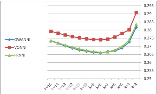
To start out with, we find the best values for the parameters used in our algorithms. These parameters are the number of neighbors, implicators, t-norms, fuzzy quantifiers, similarity measures and also OWA operators. Fortunately most of the best values have been determined before elsewhere. The best values selected for the algorithms are mentioned previously. For FRNNI and VQNNI we use the suggested values in [21]. For OWANNI we use the suggested values of parameters in [21]. The OWA operator weights are selected based on suggestions of [40]. The only parameter that must be determined is the number of neighbors, k. To find the best value for this parameter, we use 16 datasets along with 5%, 10%, 20% and 30% missing values inserted in the dataset. The tested values of k are in the range 3 to 15. Because of the lack of space we have only given the average results2. The results are illustrated in Fig. 1 to Fig. 4.

Fig. 1. Average RMSEs obtained by the algorithms on 16 datasets with 5% missing values

2

The full results can be downloaded from the following URL: http://users.aber.ac.uk/rkj/site/?page_id=745

0.22 0.23 0.24 0.25 0.26 0.27 0.28 0.29 k=3 k=4 k=5 k=6 k=7 k=8 k=9 k=10 k=11 k=12 k=13 k=14 k=15 OWANNI VQNNI FRNNI

Fig. 2. Average RMSEs obtained by the algorithms on 16 datasets with 10% missing values

Fig. 3. Average RMSEs obtained by the algorithms on 16 datasets with 20% missing values

0.22 0.23 0.24 0.25 0.26 0.27 0.28 0.29 0.3 OWANNI VQNNI FRNNI 0.23 0.24 0.25 0.26 0.27 0.28 0.29 OWANNI VQNNI FRNNI

Fig. 4. Average RMSEs obtained by the algorithms on 16 datasets with 30% missing values

The results show that for 5%, 10% and 20% missing values, while k increases, the RMSE decreases. This means that algorithms using bigger values of k perform better in terms of the obtained RMSE, although the improvement becomes less as k increases. Taking a look at the RMSEs obtained for 30% missing values reveals that the best k value for the obtained algorithms is 8. At this point all three algorithms have achieved their best RMSEs. It is worth noting that FRNNI and OWANNI perform similarly to some extent and are always better than VQNNI. Keeping in mind the aforementioned points, we have decided to choose a k value in the range 7 to 12. It is a fact that using small values of k results in a faster running time for the algorithms. But on the other hand, the obtained RMSE will be worse with small k values. Hence, it is a sensible decision not to use values of k that are too small. On the other hand, using large values for k can dramatically increase the running time of the algorithms. Furthermore, the improvement of RMSE is negligible. The suggested value for parameter k for KNNI and WKNNI is 10; hence to have a fair comparison we have decide to use k = 10 as the best value for parameter k, from now on. It is obvious that for 30% missing values, the obtained RMSE results for FRNNI, OWANNI and VQNNI may not be optimal but it is needed to have an unbiased comparison.

5.3. Comparison with other imputation methods

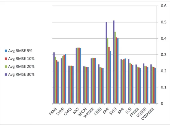
In this section, a comparison of the proposed methods with the other imputation methods is presented. The average RMSE results of the methods on 27 datasets are shown in Fig. 5.

The obtained results for 5% missing values reveal that although the proposed methods operate similarly, FRNNI regularly outperforms VQNNI. The performance of FRNNI and OWANNI are quite similar but FRNNI performs slightly better. Both of them outperform VQNNI. In comparison with the other methods, KNNI has the overall least average RMSE and therefore may be a candidate to outperform proposed methods. This will be investigated later based on the statistical tests. While the best RMSE values are less than 0.25 some of the methods have generated higher RMSEs, namely KMI, SDVI, EMI, WKNNI, MCI, SVMI and FKMI. Three of them achieved the worst results: SVDI, MCI and EMI.

Considering other amounts of missing values, it is obvious that the results are quite similar to what is obtained for 5% missing values. When the percentage of missing values rises, the RMSE raises slightly although there are some exceptions for this. SVMI exhibits an unusual behavior in that while the percentage of missing values increases, the average RMSE obtained by SVMI decreases.

0.25 0.255 0.26 0.265 0.27 0.275 0.28 0.285 0.29 0.295 OWANNI VQNNI FRNNI

Fig. 6 shows the standard deviation of the obtained average RMSEs. The standard deviation indicates how the performance of the algorithms changes with respect to the different percentages of missing values. The less standard deviation, the steadier the algorithm has performed. Some methods obtain approximately equal RMSE results for all percentages of missing values. They are KMI, WKNNI, BPCAI, MCI and CMCI. Our proposed methods have a standard deviation of about 0.01. The worst standard deviations achieved relates to EMI, followed by SVDI and FKMI. The nearest neighbor approaches would appear to be better estimators of the missing values and less variable in their imputed results.

To have a better view on how the methods performed, we have conducted Wilcoxon non-parametric statistical tests. Tables 4 to 6 show the results for FRNNI, OWANNI and VQNNI. Because of the lack of space, we have not presented the R+ and R- values. Instead the obtained p-values for the different missing values are presented.

Fig. 5. Average RMSEs obtained from the 11 missing value imputation methods on 27 datasets

0 0.1 0.2 0.3 0.4 0.5 0.6 Avg RMSE 5% Avg RMSE 10% Avg RMSE 20% Avg RMSE 30%

Fig. 6. Standard deviations of the obtained average RMSEs

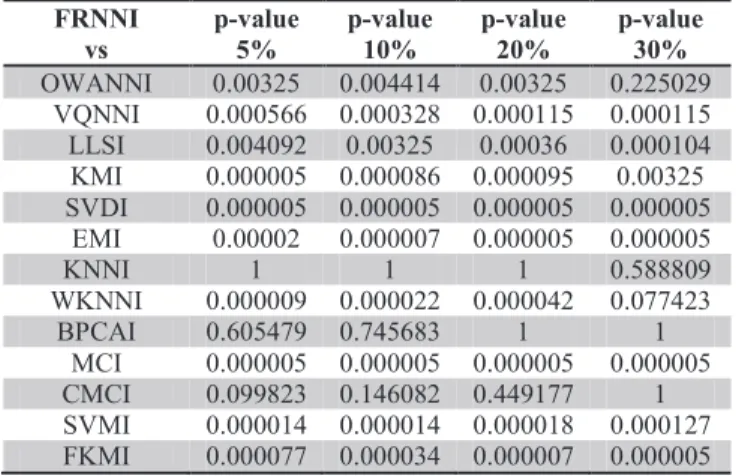
Table 4. Comparison of the imputation algorithms with FRNNI in terms of RMSE.

FRNNI vs p-value 5% p-value 10% p-value 20% p-value 30% OWANNI 0.00325 0.004414 0.00325 0.225029 VQNNI 0.000566 0.000328 0.000115 0.000115 LLSI 0.004092 0.00325 0.00036 0.000104 KMI 0.000005 0.000086 0.000095 0.00325 SVDI 0.000005 0.000005 0.000005 0.000005 EMI 0.00002 0.000007 0.000005 0.000005 KNNI 1 1 1 0.588809 WKNNI 0.000009 0.000022 0.000042 0.077423 BPCAI 0.605479 0.745683 1 1 MCI 0.000005 0.000005 0.000005 0.000005 CMCI 0.099823 0.146082 0.449177 1 SVMI 0.000014 0.000014 0.000018 0.000127 FKMI 0.000077 0.000034 0.000007 0.000005

The obtained results for FRNNI show that FRNNI outperforms most of the imputation methods. The reason is that obtained asymptotic p-values are less than the 0.1 (and often 0.05) level of significance. For example, for 5% missing values, most of the p-values are less than 0.1. Therefore it is inferred that FRNNI outperforms the other algorithms. The only exceptions are KNNI and BPCAI. The performance of the two must be determined by investigating their obtained p-values against FRNNI. With making reference to Table 7 and Table 8, it is inferred that KNNI and BPCAI perform similar to FRNNI. Hence one can infer that FRNNI outperforms most of the imputation methods and also performs as well as the best methods.

To summarize, for 5% missing values, no method outperforms FRNNI and FRNNI performs similar to KNNI and BPCAI. For 10% and 20% missing values, no method outperforms FRNNI and FRNNI performs similar to KNNI, BPCAI and CMCI. For 30% missing values, BPCAI outperforms FRNNI and FRNNI performs similar to KNNI, OWANNI and CMCI.

It is obvious that BPCAI, KNNI and CMCI are amongst the best performing methods. The reason why BPCAI outperforms FRNNI for data with 30% missing values may be as a result of the choice of parameter k. The optimum k value is 8 for 30% missing values but we have used 10 to have a fair comparison with other methods.

0 0.01 0.02 0.03 0.04 0.05 0.06 0.07 0.08 0.09

Table 5. Comparison of the imputation algorithms with OWANNI in terms of RMSE. OWANNI vs p-value 5% p-value 10% p-value 20% p-value 30% VQNNI 0.001132 0.000618 0.001863 0.00852 FRNNI 1 1 1 1 LLSI 0.011256 0.011256 0.000804 0.000154 KMI 0.000005 0.000086 0.000086 0.004759 SVDI 0.000005 0.000005 0.000005 0.000005 EMI 0.000034 0.00001 0.000005 0.000005 KNNI 1 1 1 1 WKNNI 0.000005 0.00002 0.00014 0.10487 BPCAI 0.838187 1 1 1 MCI 0.000005 0.000005 0.000005 0.000005 CMCI 0.13321 0.190412 0.478487 1 SVMI 0.000018 0.000018 0.000022 0.000187 FKMI 0.000095 0.000042 0.000008 0.000005

The obtained p-values for OWANNI reveal that it outperforms most of the existing imputation methods. The only exceptions that may perform better than OWANNI are FRNNI, KNNI, BPCAI and CMCI. To summarize: For 5%, 10% and 20% missing values, FRNNI and KNNI outperform OWANNI and OWANNI performs similar to BPCAI and CMCI. For 30% missing values, BPCAI outperforms OWANNI and OWANNI performs similar to FRNNI, WKNNI, KNNI and CMCI.

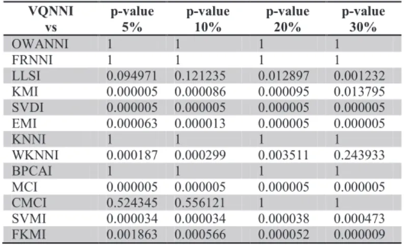
Table 6. Comparison of the imputation algorithms with VQNNI in terms of RMSE.

VQNNI vs p-value 5% p-value 10% p-value 20% p-value 30% OWANNI 1 1 1 1 FRNNI 1 1 1 1 LLSI 0.094971 0.121235 0.012897 0.001232 KMI 0.000005 0.000086 0.000095 0.013795 SVDI 0.000005 0.000005 0.000005 0.000005 EMI 0.000063 0.000013 0.000005 0.000005 KNNI 1 1 1 1 WKNNI 0.000187 0.000299 0.003511 0.243933 BPCAI 1 1 1 1 MCI 0.000005 0.000005 0.000005 0.000005 CMCI 0.524345 0.556121 1 1 SVMI 0.000034 0.000034 0.000038 0.000473 FKMI 0.001863 0.000566 0.000052 0.000009

And finally for VQNNI the following results are achieved: For 5% and 10% missing values, OWANNI, FRNNI and KNNI outperform VQNNI. VQNNI performs similar to LLSI, BPCAI and CMCI. For 20% missing values, OWANNI, FRNNI and KNNI again all outperform VQNNI. VQNNI performs similar to BPCAI and CMCI. For 30% missing values, VQNNI is outperformed by OWANNI, FRNNI, BPCAI and CMCI. VQNNI performs similar to KNNI and WKNNI. Table 9 summarizes the results.

Table 7. Comparison of the imputation algorithms with KNNI in terms of RMSE.

KNNI vs p-value 5% p-value 10% p-value 20% p-value 30% OWANNI 0.031536 0.013795 0.011256 0.605479 VQNNI 0.005128 0.010508 0.001232 0.13321 FRNNI 0.508813 0.605479 0.656708 1 LLSI 0.00104 0.00202 0.000432 0.000432 KMI 0.000005 0.000086 0.000086 0.004759 SVDI 0.000005 0.000005 0.000005 0.000005 EMI 0.000014 0.000006 0.000005 0.000005

WKNNI 0.000005 0.000005 0.000063 0.10487 BPCAI 0.478487 0.420913 0.857005 1 MCI 0.000005 0.000005 0.000005 0.000005 CMCI 0.037694 0.056135 0.225029 1 SVMI 0.000012 0.000009 0.000008 0.00014 FKMI 0.000031 0.000009 0.000005 0.000005

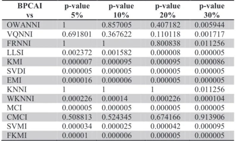
Table 8. Comparison of the imputation algorithms with BPCAI in terms of RMSE.

BPCAI vs p-value 5% p-value 10% p-value 20% p-value 30% OWANNI 1 0.857005 0.407182 0.005944 VQNNI 0.691801 0.367622 0.110118 0.001717 FRNNI 1 1 0.800838 0.011256 LLSI 0.002372 0.001582 0.000008 0.000005 KMI 0.000007 0.000095 0.000095 0.000086 SVDI 0.000005 0.000005 0.000005 0.000005 EMI 0.000016 0.000006 0.000005 0.000005 KNNI 1 1 1 0.011256 WKNNI 0.000226 0.00014 0.000226 0.000104 MCI 0.000005 0.000005 0.000005 0.000005 CMCI 0.508813 0.524345 0.674166 0.913906 SVMI 0.000034 0.000025 0.000042 0.000095 FKMI 0.00001 0.000006 0.000005 0.000005

Table 9. Summary of the findings based on statistical tests for significance level = 0.1.

Method Methods with similar performance (MV=5%)

Methods performing better (MV=5%)

OWANNI BPCAI, CMCI FRNNI, KNNI

VQNNI LLSI, BPCAI, CMCI OWANNI, FRNNI, KNNI

FRNNI KNNI, BPCAI, CMCI ---

Method Methods with similar performance (MV=10%)

Methods performing better (MV=10%)

OWANNI BPCAI, CMCI FRNNI, KNNI

VQNNI LLSI, BPCAI, CMCI OWANNI, FRNNI, KNNI

FRNNI KNNI, BPCAI, CMCI ---

Method Methods with similar performance (MV=20%)

Methods performing better (MV=20%)

OWANNI BPCAI, CMCI FRNNI, KNNI

VQNNI BPCAI, CMCI OWANNI, FRNNI, KNNI

FRNNI KNNI, BPCAI, CMCI ---

Method Methods with similar performance (MV=30%)

Methods performing better (MV=30%)

OWANNI FRNNI, KNNI, WKNNI, CMCI BPCAI

VQNNI KNNI, WKNNI OWANNI, FRNNI, BPCAI, CMCI

FRNNI OWANNI, KNNI, CMCI BPCAI