Linking resource selection and step selection models for
habitat preferences in animals
Th´
eo Michelot
1∗, Paul G. Blackwell
1, Jason Matthiopoulos
2 1University of Sheffield,
2University of Glasgow
Abstract
The research community working on species-habitat associations in animals is currently facing a paralysing methodological conundrum, because its two dominant analytical approaches have been shown to reach divergent conclusions. Models fitted from the viewpoint of an individual (step selection func-tions), once scaled up, do not agree with models fitted from a population viewpoint (resource selection functions). We explain this fundamental incompatibility, and propose a solution by introducing to the animal movement field a novel use for the well-known family of Markov chain Monte Carlo (MCMC) algorithms. By design, the step selection rules of MCMC lead to a steady-state distribution that coin-cides with a given underlying function: the target distribution. We therefore propose an analogy between the movements of an animal and the movements of an MCMC sampler, to guarantee convergence of the step selection rules to the parameters underlying the population’s utilisation distribution. We introduce a rejection-free MCMC algorithm, the local Gibbs sampler, that better resembles real animal movement, and discuss the wide range of biological assumptions that it can accommodate. We illustrate our method with simulations on a known utilisation distribution, and show theoretically and empirically that locations simulated from the local Gibbs sampler arise from the correct resource selection function.
1
Introduction
Understanding how animals use a landscape in response to its habitat composition is a crucial question in pure and applied ecology. Such insights are achievable only by confronting species-habitat association models with usage data, collected either via transect surveys or via biologging methods. Statistical inference, to link these data to environmental variables, can be approached from a population perspective, using resource selection functions (RSF; Manly et al., 2007). Alternatively, if individually referenced data (i.e. telemetry) are available, the question can be addressed from the viewpoint of the single animal, via step selection functions (SSF; Thurfjell et al., 2014). The population/individual dichotomy between these two approaches is not always clear-cut, because RSFs can be applied to the utilisation distribution of single animals, and SSFs can combine joint insights from multiple individuals. Nevertheless, the two methods roughly fall at opposite ends of the Eulerian-Lagrangian spectrum outlined by Turchin (1998). Therefore, researchers in this area have tended to think of the habitat preference parameters obtained via SSFs as the microscopic rules of movement, while the corresponding parameters of an RSF are implicitly thought of as the macroscopic patterns obtained when time is integrated out. Hence, SSF models are increasingly concerned with the geometry of movement trajectories (e.g. step lengths and turning angles in different behavioural states in Squires et al., 2013), while RSF predictions often make a pseudo-equilibrium assumption (Guisan and Thuiller, 2005), which is a biological term reminiscent of the mathematical idea of steady-state distributions. But here-in lies a fundamental problem for this entire field of statistical analysis. A correctly formulated framework of
∗Corresponding author: [email protected]
movement must work across scales, such that, when the microscopic rules of individual movement are scaled up in space and time, they give rise to the expected macroscopic distribution of a population. However, there is now both analytical (Barnett and Moorcroft, 2008; Moorcroft and Barnett, 2008) and numerical (Signer et al., 2017) evidence that the steady-state distribution generated from SSFs does not match the spatial predictions of the RSF fitted to the same data. Here, we explain how this discrepancy arises and propose a solution.
A RSF w(c) is proportional to the probability of a resource unit c being used (Boyce and McDonald, 1999). Depending on the type of usage data available, RSFs are derived in two steps. First, a model is fitted to the response and explanatory data. For example, a point process model (Aarts et al., 2012) or a use-availability logistic regression (Boyce and McDonald, 1999; Aarts et al., 2008) can be used for telemetry data, and a log-linear regression can be used on count data from regular grids or line transects. Second, irrespective of the type of response data and model fitting method, the linear predictor of the resulting statistical model is transformed via a non-negative function (Manly et al., 2007, Chapter 2), of which the most common is the exponential,
w(c) = exp(β1c1+β2c2+· · ·+βncn), (1)
where c is a vector of ncovariate values, and β1, β2, . . . , βn are the associated regression coefficients. The
RSF can be used to model the utilisation distribution π(x), i.e. the distribution of the animal’s space use,
π(x) = R exp(β1c1(x) +β2c2(x) +· · ·+βncn(x)) exp(β1c1(y) +β2c2(y) +· · ·+βncn(y))dy
, (2)
where the functions c1, c2, . . . , cn associate a spatial location xto the corresponding covariate values. The
utilisation distribution is normalized to ensure that it defines a valid probability distribution forx. Although they can encompass a wider range of environmental conditions, the covariates are often called resources in this context. In the following, we use “covariates” and “resources” interchangeably.
RSF approaches are commonly used to estimate the apparent effect of a spatial covariate on a species. The resource selection coefficientsβk characterize this effect for each of thencovariates (βk >0: preference;
βk < 0: avoidance; βk = 0: indifference). However, recent work has shown that these interpretations are
highly sensitive to the context in which the organisms are being studied, in particular, the availability of all habitat types to the animals (Beyer et al., 2010; Matthiopoulos et al., 2011; Paton and Matthiopoulos, 2016). Thus, in this framework, the definition of habitat availability, determined by assumptions of spatial accessibility (Matthiopoulos, 2003), is important in deducing preference from observed usage. For example, when using RSFs to analyse a time series of positions from a ranging animal, it may not be plausible to assume that all locations in the home range are accessible by the animal at every step (Northrup et al., 2013). RSF approaches are often forced to treat such non-independence as a statistical nuisance (Aarts et al., 2008; Fieberg et al., 2010), but step selection approaches treat it as an asset.
In step selection analyses, the likelihoodp(y|x) of a potential displacement by the animal to a locationy
over a given time interval (typically, the sampling interval) is modelled in terms of the habitat composition in the neighbourhood of the animal’s current positionx:
p(y|x) = R φ(y|x)w(c(y))
φ(z|x)w(c(z))dz, (3)
where φ(·|x) is the resource-independent movement kernel around x (Rhodes et al., 2005; Forester et al., 2009) and, for any location x, c(x) = (c1(x), c2(x), . . . , cn(x)). To link the movement to environmental
covariates, w is modelled using the same log-linear link as the RSF, given in Equation 1. The term “step selection function” (SSF) is most often used forw(e.g. by Fortin et al., 2005; Thurfjell et al., 2014); however, note that it is sometimes used for the whole numerator in the right-hand side of Equation 3 (see Forester et al., 2009). In the following, we callwthe SSF.
The choice of the functionφcharacterizes accessibility, and hence determines availability, in a step selection model; it corresponds to the distribution of feasible steps over one time interval, with origin x, when the
resources do not affect the movement. It can, for example, be a uniform distribution on a disc around the current location x (e.g. the availability model of Rhodes et al., 2005), or obtained from the empirical distributions of movement metrics (e.g. step lengths and turning angles in Fortin et al., 2005).
SSFs are most often fitted using conditional logistic regression on matched use-availability data, where each observed stepxt→xt+1 is matched to a set of random steps generated fromφ(·|xt) (Thurfjell et al.,
2014).
Duchesne et al. (2015) showed that a step selection model defines a movement model equivalent to a biased correlated random walk (BCRW). BCRWs are routinely used in ecology as a flexible basis for models of individual movement (Turchin, 1998; Codling et al., 2008). Avgar et al. (2016) extended the step selection approach to allow the simultaneous estimation of the step selection coefficients and of parameters of the movement model (e.g. parameters of the distributions of step lengths and turning angles), making it a very attractive framework to draw inference on habitat preference from movement data. Step selection models have been used to analyse the impact of landscape features on animal space use (e.g. Coulon et al., 2008; Roever et al., 2010), as well as animal interactions (Potts et al., 2014).
Although the RSF and SSF are typically described with the same notation, and used for the same purpose of estimating habitat preference, it can be shown that their steady-state predictions do not generally coincide. For a known utilisation distribution, Signer et al. (2017) simulated from a fitted SSF, and showed empirically that the distribution of simulated movement differed from the utilisation distribution. In particular, the difference was greater whenφwas narrow compared to the scale of habitat features. Similarly, Barnett and Moorcroft (2008) showed that, for the step selection model defined in Equation 3, the steady-state distribution of the animal’s location (i.e. its utilisation distribution) is given by
π(x) = w(c(x)) R w(c(y))φ(y|x)dy R w(c(y))R w(c(z))φ(z|y)dzdy. (4)
That is, the steady-state distribution of the model is generally not proportional to the SSF w, and that discrepancy crucially depends on the choice of the resource-independent movement kernel φ. An example of this is their earlier result (Moorcroft and Barnett, 2008) that under one specific set of assumptions, the steady-state distribution is approximately proportional to thesquare of the SSF.
Although it may seem disconcerting that the two approaches lead to different estimates ofw, the cause of this apparent paradox is partly due to the notational misuse of the same symbol for what are, in effect, different objects. The SSF captures local aspects of the animal’s movement, because it only considers a neigh-bourhood of the current location of the animal (determined byφ) and only becomes a better approximation of the RSF when the scale ofφincreases (Barnett and Moorcroft, 2008). The parameters of the two objects coincide in the limiting case of unconstrained mobility, i.e. when the availability assumed by both methods is global. However, in every other case, the two methods are indeed different.
Rather than seeking an equivalence of the parameters estimated by the two methods, and attempting to impose on them the same biological interpretation, a better question to ask is: under what assumptions do the parameters estimated by a SSF model lead to movement that scales to the distribution yielded by the parameters of a RSF model? We answer this question by describing a new model of step selection, that scales correctly to the steady-state distribution captured by the RSF. In Section 2, we reconcile resource selection and step selection conceptually, with a model of animal movement for which the long-term distribution of locations is guaranteed to be proportional to the RSF. Our method uses an analogy between the movement of an animal in geographical space and the movement of a Markov Chain Monte Carlo (MCMC) sampler in its parameter space. In Section 3, we make these concepts applicable in practice, by developing a family of MCMC algorithms with considerable potential for encompassing realistic movement assumptions. In Section 4, we illustrate our method using simulations on a known utilisation distribution, and verify that the dis-tribution of simulated locations corresponds to the correct RSF. In Section 5, we discuss the rich diversity of MCMC samplers that could be used to accommodate increasingly realistic features of movement into the modelling.
2
A model of step selection using a movement-MCMC analogy
MCMC methods are a general framework to sample from a probability distribution, termed the target distribution (Gilks et al., 1995). This approach is mostly used for Bayesian inference, to sample from the (posterior) distribution of a set of unknown parameters (Gelman et al., 2014, Chapter 11). It includes a very wide class of algorithms, among them the widely-used Metropolis-Hastings and Gibbs samplers. A MCMC algorithm describes the steps to generate a sequence of points x1,x2,x3. . ., whose long-term distribution is the target distribution. Each MCMC algorithm is defined by its transition kernel p(xt+1|xt), which
determines (for any t = 1,2, . . .) how the point xt+1 should be sampled, given xt. For example, in a
Metropolis-Hastings algorithm, the transition kernel is a combination of the proposal distribution and the acceptance probability:
p(xt+1|xt) =p(xt+1is proposed|xt)×p(xt+1 is accepted|xt).
In general, given some easily-satisfied technical conditions, a sufficient condition forp(xt+1|xt) to define
a valid MCMC algorithm for the target distribution π (i.e. to ensure that the distribution of samples will converge to π) is the detailed balance condition:
∀x,y, π(y)p(x|y) =π(x)p(y|x). (5)
That is, if the process is in equilibrium with distributionπ, then the rates of moves in each direction between any xandy balance out.
We propose an analogy between an animal’s observed movement inn-dimensional geographical space, and the movement of a MCMC sampler in a n-dimensional parameter space, for which the target distribution is the utilisation distribution. That is, we consider that a tracked animal “samples” spatial locations in the short term from some movement model, and in the long run from its utilisation distribution, in the same way that a MCMC algorithm samples points in the short term from some transition kernel and in the long term from its target distribution. A MCMC algorithm then defines a movement model, for which the steady-state distribution is known.
The utilisation distribution can be modelled with the RSF, as defined in Equation 2, to link the target distribution of the movement model to the distribution of resources.
Thus the movement processxtis defined as follows. Choose a MCMC algorithm for the target distribution
π(the normalized RSF), with transition kernelp(xt+1|xt). Start from a pointx1. Fort= 1,2, . . ., the next locationxt+1 is sampled fromp(xt+1|xt). By property of MCMC samplers, the steady-state distribution for
xtisπ.
In this framework, the choice of the MCMC algorithm determines the movement model. For example, with a Metropolis-Hastings model, different proposal distributions might capture different features of the animal’s movement. The parameters of the algorithm, which are usually regarded as tuning parameters, are here parameters of the movement process. For example, the variance of the proposal distribution could be a measure of the animal’s speed. It is important to make a distinction between these parameters of movement, and the parameters of the target distribution (i.e. the resource selection parameters). Two different samplers might have the same target distribution, but the rate at which it is approached by the MCMC samples will depend on the choice of algorithm. Indeed, part of the success of MCMC in its Bayesian context is the flexibility in choosing the transition kernel for a given target distribution. In particular, for our application, we want an algorithm corresponding to a realistic model of movement, in addition to having the correct target distribution. Rejection-based MCMC algorithms (such as Metropolis-Hastings) might seem to be an unnatural choice to model animal movement, because there are typically no rejections in telemetry data:
the animals will always change position in the process of sampling a new candidate location. As such, the tracking data would be considered an exceptional – although not impossible – output for a classic MCMC algorithm. To circumvent this problem, we design a rejection-free MCMC algorithm in Section 3.
3
The local Gibbs sampler
Metropolis-Hastings samplers require a rejection step to ensure convergence to the target distribution. View-ing this as a movement model implies the unlikely scenario of a return by the animal to its previous position, after having tested and rejected a relocation. Instead, it is more natural to think about tracking data as the outcome of a rejection-free sampler. Here, we describe such an algorithm, that we call the local Gibbs sampler.
In the classic Gibbs sampler, each ‘step’ involves updating just one of the n parameters, xj say, while
keepingx1, . . . , xj−1, xj+1, . . . , xnfixed; the values ofjcan be chosen systematically or randomly. Thus each
step is a move within a one-dimensional ‘slice’ of the parameter space, rather than over the whole space. It is used when the target distribution over each such one-dimensional slice (the so-called ‘full conditional distribution’) is mathematically tractable and so can be used as the transition kernel for that step without the need for any accept/reject stage.
The local Gibbs sampler uses the same idea of sampling from a restricted part of the target distribution: at each iteration t, the updated parameter xt+1 is sampled directly from the target distribution, truncated to some neighbourhood of xt. The way in which this neighbourhood is selected is crucial to ensuring that
the algorithm samples from the required target distribution in the long run.
In explaining the details of the algorithm, we assume that n = 2, by far the most important case for ecological applications, though the algorithm works for any nwith straightforward changes. For any point
x, andr >0, we defineDr(x) to be the disc of centrexand radiusr.
The local Gibbs sampler forπis given by the following steps. The track starts from a locationx1, and moves to locationsxt+1 over iterationst= 1,2, . . ..
1. On iterationt, sample a pointz uniformly from the discDr(xt).
2. Define ˜πthe truncated distribution,
˜ π(y) = ( π(y)/Cr(z) ify∈ Dr(z), 0 elsewhere, whereCr(z) =Ry∈D r(z)π(y)dyis a normalizing constant.
3. Sample the next locationxt+1according to the constrained likelihood ˜π.
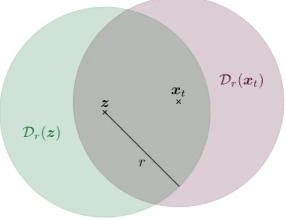
The notation is illustrated in Figure 1. The local Gibbs sampler has one parameter: the radius r >0 of the relocation disc. Here, for simplicity, we only consider the case where r is fixed, but the algorithm would still work ifrwere generated at each iteration from a probability distribution. Taking the local Gibbs algorithm as a movement model, the parameter r defines the scale of the animal’s perception range and, indirectly, the scale of its movement.
Taking π to be the normalized RSF (Equation 2), the local Gibbs algorithm defines a step selection (movement) model in which the distribution of the animal’s space use is guaranteed to be proportional to
r
Dr(z)
Dr(xt)
xt
z
Figure 1: Notation for the local Gibbs sampler in two dimensions. The pointzis sampled uniformly fromDr(xt), and the next locationxt+1is sampled from the RSF truncated toDr(z).
the RSF. Indeed, it satisfies the detailed balance condition (Equation 5): givenr, we have
π(x)p(y|x) =π(x) Z z∈Dr(x) p(y|z)p(z|x)dz =π(x) Z z∈Dr(x) π(y) Cr(z) 1 πr2I{y∈Dr(z)}dz = π(x)π(y) πr2 Z z∈Dr(x)∩Dr(y) 1 Cr(z) dz =π(y)p(x|y) by symmetry.
The local Gibbs model is superficially similar to the availability radius model of Rhodes et al. (2005) and the uniform sampling step selection model of Forester et al. (2009). In those models, at each time step, the next locationxt+1is sampled from the RSF truncated and scaled on a disc centred onxt. That is, in step 1
of the algorithm described above, they takez=xt. This means that there is no mechanism in their approach
to guarantee that the overall distribution of the sampled locations is the RSF. Specifically, the two sides of the detailed balance equation involve different normalization constants, and so their movement models do not have the normalized RSF as their equilibrium distributions. For this reason, it is not clear how the coefficients they estimate should be interpreted, and how they differ from the resource selection coefficients estimated from a RSF approach.
The local Gibbs algorithm can be used to simulate tracks on a known RSF. The truncation of the RSF to the discDr(z) requires the calculation of the normalizing constant Cr(z). It is not generally possible to
derive it analytically, but Monte Carlo sampling can be used to estimate it. In practice, to sample from the truncated target distribution ˜π,ndpoints are generated uniformly inDr(z), andxt+1is sampled from those points, with probabilities proportional to their RSF values. Simulation using the local Gibbs algorithm is illustrated in Figure 2.
We can derive the corresponding resource-independent movement kernelφLG(y|x), to describe the distri-bution of steps on a flat target distridistri-bution. In the case where ris fixed,
φLG(y|x) = 1 (πr2)2A(Dr(x)∩ Dr(y)) ifky−xk ≤2r, 0 otherwise, (6)
−10 0 10 −10 0 10 x y 10 20 30 RSF
Figure 2: Illustration of the local Gibbs sampler in two dimensions. The background is the RSF; the solid line is the simulated track up to timet; the red cross is the current locationxt; the red circle delimitsDr(z). The next location
xt+1is sampled from the black dots, with probabilities proportional to their RSF values.
the discs of centres x andy, and of radius r. The point z is such that kz−xk< r andkz−yk< r, and so – in the absence of environmental effects – the relative probability of a step fromx toy is proportional to A(Dr(x)∩ Dr(y)). By construction, it is impossible to have a step between two points if the distance
between them is larger than 2r, henceφLG(y|x) = 0 whenky−xk>2r. The detail of the derivation is given in Appendix A.
4
Simulations
We illustrate the method described in Section 2, with the local Gibbs sampler. We show that our algorithm can produce movement tracks on a known utilisation distribution. The R code used for the simulations is available on request.
4.1
Simulated resources
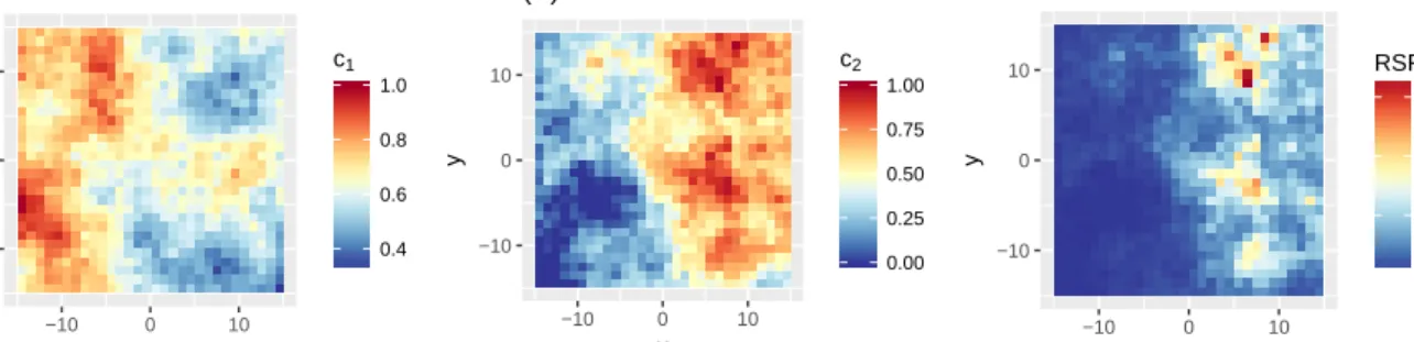
To mimic the type of environmental data of a real case study, we simulated two covariate distributions c1 and c2 as Gaussian random fields on square cells of side 1, using the R package gstat (Pebesma, 2004). We restricted the study region to Ω = [−15,15]×[−15,15], to ensure that the target distribution is integrable. Plots ofc1 andc2 are shown in Figure 3(A) and 3(B). The utilisation distribution is defined by
π(x) = R exp(β1c1(x) +β2c2(x)) y∈Ωexp(β1c1(y) +β2c2(y))dy
,
withβ1=−1 andβ2= 4 (i.e. avoidance forc1and preference forc2). A plot of the RSF is shown in Figure 3(C).
−10 0 10 −10 0 10 x y 0.4 0.6 0.8 1.0 c1 (A) −10 0 10 −10 0 10 x y 0.00 0.25 0.50 0.75 1.00 c2 (B) −10 0 10 −10 0 10 x y 10 20 30 RSF (C)
Figure 3: Resource distributionsr1 (A) andr2 (B), and RSF (C), for the simulations.
4.2
Local Gibbs simulation
The algorithm described in Section 3 can be used to simulate a movement track on a given target distribution. We considered the utilisation distribution π defined in Section 4.1. To analyse the behaviour of the local Gibbs sampler at different spatial scales, we ran three simulations, with three different values for the radius
r of the movement kernel: r = 0.5,r= 2, and r= 8. The value ofr affects the range of perception of the animal and, indirectly, its speed. For each, 5×10⁵ locations were sampled with the local Gibbs algorithm, starting from the pointx1= (0,0). (Given the length of the simulated tracks, the choice of the starting point only has a minor impact on the overall distribution of sampled locations.)
For comparison, we also sampled a movement track from a step selection model with uniform sampling, as defined by Forester et al. (2009), that we denote SSFunif. For the same distributionπ, we simulated 5×10⁵ locations from SSFunif, as follows. We started from x1 = (0,0). Then, at each time step t = 1,2, . . ., we generated 100 proposed locations{p1,p2, . . . ,p100}uniformly from a disc of radiusr= 3 centred onxt. The
next locationxt+1 was sampled from the proposed locations, with each pointpi having a probability to be
picked proportional toπ(pi). Here, we choser= 3 because it gave rise to approximately the same mean step
length as the local Gibbs sampler withr= 2 (i.e. comparable speed of spatial exploration).
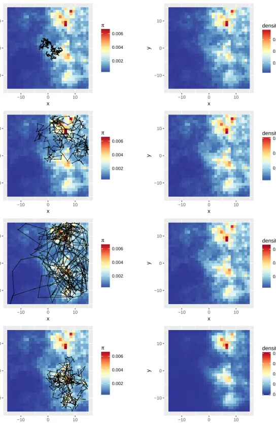
The first 300 steps of each simulated track, and the density of all simulated points, are shown in Figure 4. The density of points simulated from the local Gibbs sampler (right column, first three plots) displays the same patterns as the true RSF (Figure 3(C)). By contrast, the density of the locations obtained in the SSFunif simulation (right column, last plot) fails to capture many features of the landscape, as the process spends a disproportionate amount of time in areas of high utilisation.
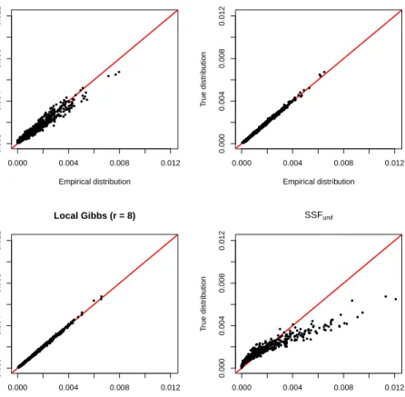
To compare the empirical distribution of simulated points to the true utilisation distribution, we plotted the (normalized) count of locations simulated in each grid cell against the corresponding utilisation value. The comparison is presented in Figure 5. Alignment with the identity line indicates similarity between the empirical and true distributions. For the three local Gibbs simulations, the points align well with the identity line – in particular in the experiments with r = 2 and r = 8, in which the speed of spatial exploration is higher than when r= 0.5. This confirms that the local Gibbs algorithm can sample movement trajectories on a given target distribution. It defines a movement model for which the long-term distribution of locations is known. However, the plot for the SSFunif simulation reveals a clearly non-linear relationship between the density of simulated points and the utilisation distribution. This result confirms the findings of Signer et al. (2017): step selection functions do not generally measure space use. We illustrated how the local Gibbs sampler circumvents this limitation of standard step selection models.
● ●● ●● ●● ● ● ● ● ● ● ● ● ● ● ● ● ● ●● ● ●● ● ● ●● ● ● ●● ● ● ● ● ● ●● ● ●● ●● ● ● ● ● ● ● ●●● ●● ● ● ● ● ● ● ● ●● ● ● ●● ● ● ● ●● ● ● ● ●●●●●● ●● ● ●●●●● ● ●● ● ● ●● ● ●● ●● ● ● ●● ● ● ●● ● ● ● ● ● ●●● ●● ● ●● ● ● ● ● ●●● ● ● ● ●●● ● ●● ● ●● ●●●● ● ●●● ● ●● ● ●●●●● ● ●● ● ●●● ●● ●●● ●●● ● ●●● ● ● ● ● ●● ● ● ●● ● ●●●● ● ● ● ● ● ● ● ● ● ● ●●● ●● ●● ● ● ● ●●●● ● ●● ● ● ● ● ● ● ● ● ● ● ● ●● ● ●●● ●● ● ● ● ● ●● ● ● ●● ● ● ●●●●●●● ● ● ● ● ● ● ●● ● ● ●● ● ● ●●● ● ● ● ●● ●●● ● ●● ● ● ●●●●●● ● ● ● ● ● −10 0 10 −10 0 10 x y 0.002 0.004 0.006 π −10 0 10 −10 0 10 x y 0.002 0.004 0.006 density ● ● ● ● ● ●● ● ● ● ● ● ● ● ● ●● ● ●● ● ● ● ● ●● ● ●●● ● ● ● ● ● ● ● ● ● ● ● ●● ● ● ● ● ● ● ● ● ● ● ● ● ● ● ● ● ● ● ● ● ● ● ● ● ● ● ● ● ● ● ● ● ● ● ● ● ● ● ● ● ● ● ● ● ● ● ●● ● ● ● ● ● ● ● ● ● ● ● ● ● ● ● ● ● ● ● ● ●●● ● ● ● ● ● ● ●● ● ● ● ● ● ● ● ● ● ● ● ● ● ●● ● ●● ● ● ● ● ● ● ● ● ● ● ● ● ● ● ● ● ● ● ●● ● ● ● ● ● ● ● ● ● ● ●● ● ● ● ● ● ● ● ● ● ● ● ● ● ● ● ● ● ● ● ● ● ● ● ● ● ● ● ● ● ● ● ● ● ● ● ● ● ● ● ● ● ● ● ● ● ● ● ● ● ● ● ● ● ● ● ● ● ● ● ● ● ● ● ● ● ● ● ● ● ● ●● ● ● ● ● ● ●● ● ● ● ● ● ● ● ● ● ● ● ●● ● ● ● ● ● ●● ● ● ● ● ● ● ● ● ● ●● ● ● ● ● ● ●● ● ● ● ● ● ● ● ● ● ● ● −10 0 10 −10 0 10 x y 0.002 0.004 0.006 π −10 0 10 −10 0 10 x y 0.002 0.004 0.006 density ● ● ● ● ● ● ● ● ● ● ● ● ● ● ● ● ● ● ● ● ● ● ● ● ● ● ● ● ● ● ● ● ● ● ● ● ● ● ● ● ● ● ● ● ● ● ● ● ● ● ● ● ● ● ● ● ● ● ● ● ● ● ● ● ● ● ● ● ● ● ● ● ● ● ● ● ● ● ● ● ● ● ● ● ● ● ● ● ● ● ● ● ● ● ● ● ● ● ● ● ● ● ● ● ● ● ● ● ● ● ● ● ● ● ● ● ● ● ● ● ● ● ● ● ● ● ● ● ● ● ● ● ● ● ● ● ● ● ● ● ● ● ● ● ● ● ● ● ● ● ● ● ● ● ● ● ● ● ● ● ● ● ● ● ● ● ● ● ● ● ● ● ● ● ● ● ● ● ● ● ● ● ● ● ● ● ● ● ● ● ● ● ● ● ● ● ● ● ● ● ● ● ● ● ● ● ● ● ●● ● ● ● ● ● ● ● ● ● ● ● ● ● ● ● ● ● ● ● ● ● ● ● ● ● ● ● ● ● ● ● ● ● ● ● ● ● ● ● ● ● ● ● ● ● ● ● ● ● ● ● ● ● ● ● ● ● ● ● ● ● ● ● ● ● ● ● ● ● ● ● ● ● ● ● ● ● ● ● ● ● ● ● ● ● ● ● ● ● ● −10 0 10 −10 0 10 x y 0.002 0.004 0.006 π −10 0 10 −10 0 10 x y 0.002 0.004 0.006 density ● ● ● ● ● ● ● ● ● ● ● ●● ● ● ● ● ● ● ● ● ● ● ● ● ● ● ● ● ● ● ● ● ● ● ● ● ● ● ● ● ● ● ● ● ● ● ● ● ● ● ● ●● ● ●● ● ● ● ● ● ● ● ● ● ● ● ● ● ● ● ● ● ● ● ● ● ● ● ● ● ● ● ●● ● ● ● ● ● ● ● ●●● ● ● ● ● ● ● ● ● ● ● ●● ● ● ● ● ● ● ● ● ● ● ● ● ● ● ● ● ● ● ● ● ● ● ● ● ● ● ● ● ● ● ● ● ● ● ● ●● ● ● ● ● ● ● ● ● ● ● ● ●● ● ● ● ● ● ● ● ● ● ● ● ● ●● ● ● ● ● ● ● ● ● ● ● ● ●● ● ● ● ● ● ● ● ● ● ● ● ● ● ● ● ● ● ● ● ● ● ● ● ● ● ● ● ● ● ● ● ● ● ● ● ● ● ● ● ● ● ● ● ● ● ● ● ● ● ● ● ● ● ●● ● ● ● ● ● ● ● ● ● ● ● ● ● ● ● ● ● ● ●● ● ● ● ● ● ● ● ● ● ● ● ● ● ● ● ● ● ● ● ● ● ● ● ● ● ● ● ● ● ● ● ● ● ● ● ● ● ● ● ● −10 0 10 −10 0 10 x y 0.002 0.004 0.006 π −10 0 10 −10 0 10 x y 0.000 0.003 0.006 0.009 0.012 density
Figure 4: Simulation using a local Gibbs sampler, with radius parameterr= 0.5(first row),r= 2(second row), and r= 8(third row); and simulation using a step selection function with uniform sampling (r=3, fourth row). The left column displays the first 300 simulated steps, and the background colour represents the utilisation distribution (i.e. the normalized RSF; the RSF is given in Figure 3(C)). The right column shows the density of the5×105 simulated locations, i.e. the normalized counts.
0.000 0.004 0.008 0.012 0.000 0.004 0.008 0.012 Local Gibbs (r = 0.5) Empirical distribution T rue distr ib ution 0.000 0.004 0.008 0.012 0.000 0.004 0.008 0.012 Local Gibbs (r = 2) Empirical distribution T rue distr ib ution 0.000 0.004 0.008 0.012 0.000 0.004 0.008 0.012 Local Gibbs (r = 8) Empirical distribution T rue distr ib ution 0.000 0.004 0.008 0.012 0.000 0.004 0.008 0.012 SSFunif Empirical distribution T rue distr ib ution
Figure 5: Results of the simulations. In each plot, the distribution of simulated points (on the x-axis) is compared to the true utilisation distribution (on the y-axis). The closer the points are to the identity line, the more similar the distributions are. In the local Gibbs simulations, the empirical distributions are very similar to the utilisation distribution; the similarity increases withr, because a larger radius leads to faster spatial exploration. For the SSFunif model, there is a clear discrepancy between the true and empirical distributions.
5
Discussion
We have presented a versatile class of models of animal movement, for which the steady-state distribution of locations is proportional to the same resource selection function that influences short-term movement. Our approach remedies a well-known shortcoming of step selection models, and reconciles the resource selection and step selection approaches to the analysis of space use data. This method shows great promise for the estimation of movement and resource selection parameters from observed animal movement data. Considering the MCMC algorithm as a movement model, it is in principle straightforward to express the likelihood of observed steps, given the parameters of the sampler (e.g. radiusrin the local Gibbs model) and of the RSF. In cases where the transition kernel of the chosen sampler,p(xt+1|xt), can be calculated, the likelihood ofT
observations x1,x2, . . . ,xT is derived asLT =Q T−1
t=1 p(xt+1|xt). Maximum likelihood estimation, or other
likelihood-based methods, can then be used to estimate simultaneously the parameters of the movement process and of the RSF. This modelling framework thus combines some of the advantages of process-based movement models and of distribution-based resource selection models. It takes us one step closer to building the crucial bridge between individual animal movement and population distribution. In addition, since individual observations of locations follow the same stationary distribution, this framework gives a coherent way to combine movement data from telemetry with independent location data arising in other ways (e.g. survey data).
Because it builds on the very wide and flexible class of MCMC samplers, various other movement al-gorithms could be considered. Models of animal movement often incorporate directional persistence, such as the discrete-time and continuous-time correlated random walks (e.g., Jonsen et al., 2005; Johnson et al., 2008, respectively). Within the framework we described, this feature of movement could be modelled using non-reversible MCMC samplers, which often display this type of autocorrelation (e.g. Michel and S´en´ecal, 2017). Such algorithms could be used for more realistic movement models.
In conclusion, most currently-used step selection models are not designed to predict space use, leading to difficulties in their interpretation. We think that MCMC algorithms can be used as models of animal movement, and reconcile resource selection and step selection approaches. Future work will be needed to develop inferential methods within this framework.
References
Aarts, G., Fieberg, J., and Matthiopoulos, J. (2012). Comparative interpretation of count, presence–absence and point methods for species distribution models. Methods in Ecology and Evolution, 3(1):177–187. Aarts, G., MacKenzie, M., McConnell, B., Fedak, M., and Matthiopoulos, J. (2008). Estimating space-use
and habitat preference from wildlife telemetry data. Ecography, 31(1):140–160.
Avgar, T., Potts, J. R., Lewis, M. A., and Boyce, M. S. (2016). Integrated step selection analysis: bridging the gap between resource selection and animal movement.Methods in Ecology and Evolution, 7(5):619–630. Barnett, A. H. and Moorcroft, P. R. (2008). Analytic steady-state space use patterns and rapid computations
in mechanistic home range analysis. Journal of mathematical biology, 57(1):139–159.
Beyer, H. L., Haydon, D. T., Morales, J. M., Frair, J. L., Hebblewhite, M., Mitchell, M., and Matthiopoulos, J. (2010). The interpretation of habitat preference metrics under use–availability designs. Philosophical Transactions of the Royal Society of London B: Biological Sciences, 365(1550):2245–2254.
Boyce, M. S. and McDonald, L. L. (1999). Relating populations to habitats using resource selection functions.
Trends in Ecology & Evolution, 14(7):268–272.
Codling, E. A., Plank, M. J., and Benhamou, S. (2008). Random walk models in biology. Journal of the Royal Society Interface, 5(25):813–834.
Coulon, A., Morellet, N., Goulard, M., Cargnelutti, B., Angibault, J.-M., and Hewison, A. M. (2008). Inferring the effects of landscape structure on roe deer (capreolus capreolus) movements using a step selection function. Landscape Ecology, 23(5):603–614.
Duchesne, T., Fortin, D., and Rivest, L.-P. (2015). Equivalence between step selection functions and biased correlated random walks for statistical inference on animal movement. PloS one, 10(4):e0122947.
Fieberg, J., Matthiopoulos, J., Hebblewhite, M., Boyce, M. S., and Frair, J. L. (2010). Correlation and studies of habitat selection: problem, red herring or opportunity? Philosophical Transactions of the Royal Society of London B: Biological Sciences, 365(1550):2233–2244.
Forester, J. D., Im, H. K., and Rathouz, P. J. (2009). Accounting for animal movement in estimation of resource selection functions: sampling and data analysis. Ecology, 90(12):3554–3565.
Fortin, D., Beyer, H. L., Boyce, M. S., Smith, D. W., Duchesne, T., and Mao, J. S. (2005). Wolves influence elk movements: behavior shapes a trophic cascade in yellowstone national park. Ecology, 86(5):1320–1330. Gelman, A., Carlin, J. B., Stern, H. S., and Rubin, D. B. (2014).Bayesian data analysis, volume 2. Chapman
& Hall/CRC Boca Raton, FL, USA.
Gilks, W. R., Richardson, S., and Spiegelhalter, D. (1995). Markov chain Monte Carlo in practice. CRC press.
Guisan, A. and Thuiller, W. (2005). Predicting species distribution: offering more than simple habitat models. Ecology letters, 8(9):993–1009.
Johnson, D. S., London, J. M., Lea, M.-A., and Durban, J. W. (2008). Continuous-time correlated random walk model for animal telemetry data. Ecology, 89(5):1208–1215.
Jonsen, I. D., Flemming, J. M., and Myers, R. A. (2005). Robust state–space modeling of animal movement data. Ecology, 86(11):2874–2880.
Manly, B., McDonald, L., Thomas, D., McDonald, T. L., and Erickson, W. P. (2007). Resource selection by animals: statistical design and analysis for field studies. Springer Science & Business Media.
Matthiopoulos, J. (2003). The use of space by animals as a function of accessibility and preference.Ecological Modelling, 159(2):239–268.
Matthiopoulos, J., Hebblewhite, M., Aarts, G., and Fieberg, J. (2011). Generalized functional responses for species distributions. Ecology, 92(3):583–589.
Michel, M. and S´en´ecal, S. (2017). Forward event-chain monte carlo: a general rejection-free and irreversible markov chain simulation method. arXiv preprint arXiv:1702.08397.
Moorcroft, P. R. and Barnett, A. (2008). Mechanistic home range models and resource selection analysis: a reconciliation and unification. Ecology, 89(4):1112–1119.
Northrup, J. M., Hooten, M. B., Anderson, C. R., and Wittemyer, G. (2013). Practical guidance on character-izing availability in resource selection functions under a use–availability design. Ecology, 94(7):1456–1463. Paton, R. S. and Matthiopoulos, J. (2016). Defining the scale of habitat availability for models of habitat
selection. Ecology, 97(5):1113–1122.
Pebesma, E. J. (2004). Multivariable geostatistics in s: the gstat package. Computers & Geosciences, 30(7):683–691.
Potts, J. R., Mokross, K., and Lewis, M. A. (2014). A unifying framework for quantifying the nature of animal interactions. Journal of The Royal Society Interface, 11(96):20140333.
Rhodes, J. R., McAlpine, C. A., Lunney, D., and Possingham, H. P. (2005). A spatially explicit habitat selection model incorporating home range behavior. Ecology, 86(5):1199–1205.
Roever, C. L., Boyce, M. S., and Stenhouse, G. B. (2010). Grizzly bear movements relative to roads: application of step selection functions. Ecography, 33(6):1113–1122.
Signer, J., Fieberg, J., and Avgar, T. (2017). Estimating utilization distributions from fitted step-selection functions. Ecosphere, 8(4).
Squires, J. R., DeCesare, N. J., Olson, L. E., Kolbe, J. A., Hebblewhite, M., and Parks, S. A. (2013). Combining resource selection and movement behavior to predict corridors for canada lynx at their southern range periphery. Biological Conservation, 157:187–195.
Thurfjell, H., Ciuti, S., and Boyce, M. S. (2014). Applications of step-selection functions in ecology and conservation. Movement ecology, 2(1):4.
Turchin, P. (1998). Quantitative Analysis of Movement: Measuring and Modeling Population Redistribution in Animals and Plants. Beresta Books.
Appendix
Appendix A. Movement kernel for the local Gibbs model
For a fixed radius rand any target distributionπ, we havep(xt+1|xt) = Z z∈Dr(xt) p(xt+1|z)p(z|xt)dz = Z z∈Dr(xt) π(xt+1)I{xt+1∈Dr(z)} R y∈Dr(z)π(y)dy 1 πr2dz = 1 πr2 Z z∈D(rt) π(xt+1) R y∈Dr(z)π(y)dy dz,
where D(rt)=Dr(xt)∩ Dr(xt+1), andI is the indicator function. Then, if the target distribution is flat, say
∀x, π(x) =k, we have p(xt+1|xt) = 1 πr2 Z z∈D(rt) k R y∈Dr(z)k dy dz = k πr2 Z z∈D(rt) 1 kπr2dz = 1 (πr2)2 Z z∈D(rt) dz = 1 (πr2)2A(D (t) r )
where A(D(rt)) is the area ofD
(t)
r . It can be shown that
A(D(t) r ) = 2r 2cos−1 d t 2r −dt r r2−d 2 t 4 where dt=kxt+1−xtkis the distance betweenxtandxt+1.