Frequency Domain Estimation of Cointegrating
Vectors with Mixed Frequency and
Mixed Sample Data
Marcus J. Chambers
University of Essex
January 2018
Abstract
This paper proposes a model suitable for exploiting fully the information contained in mixed frequency and mixed sample data in the estimation of cointegrating vectors. The asymptotic properties of easy-to-compute spectral regression estimators of the cointegrating vectors are derived and these estimators are shown to belong to the class of optimal cointegration esti-mators. Furthermore, Wald statistics based on these estimators have asymptotic chi-square distributions which enable inferences to be made straightforwardly. Simulation experiments suggest that the finite sample performance of a spectral regression estimator in an aug-mented mixed frequency model is particularly encouraging as it is capable of dramatically reducing the root mean squared error obtained in an entirely low frequency model to the levels comparable to an infeasible high frequency model. The finite sample size and power properties of the Wald statistic are also found to be good. An empirical example, to stock price and dividend data, is provided to demonstrate the methods in practice.
Keywords: mixed frequency data; mixed sample data; cointegration; spectral regression.
J.E.L. classification number: C32.
Acknowledgements: I thank participants at the 10th York Econometrics Symposium, University of York, 15–16 June, 2017, for helpful comments on an earlier version of this piece of work, as well as attendees at the session on ‘Co-integration, trend breaks, and mixed frequency data’ at the 11th International Conference on Computational and Finan-cial Econometrics, Senate House, University of London, 16–18 December, 2017. Finan-cial support provided by the Economic and SoFinan-cial Research Council under grant number ES/M01147X/1 is gratefully acknowledged.
Address for Correspondence: Marcus J. Chambers, Department of Economics, Univer-sity of Essex, Wivenhoe Park, Colchester, Essex CO4 3SQ, England.
1. Introduction
The concept of cointegration plays a prominent role in the analysis of multivariate time series with unit roots, and a large variety of methods is available to the applied researcher for handling such data. Prominent among these methods is the vector error correction model (VECM) which is a convenient reparameterisation of a vector autoregressive (VAR) system that accounts for the cointegration between the variables. The popularity of the fully para-metric VECM approach – often termed the ‘Johansen’ approach following its development by Johansen (1991) – lies in its (relative) ease of estimation and its suitability for testing for the number of cointegrating vectors that exist. The VECM method is also implemented in many econometric software packages, is amenable to use as a forecasting tool and can be subjected to the usual battery of time series specification tests.
In some circumstances, however, a researcher may be unwilling to model the system dynamics in the form of a VAR, which is often heavily parameterised, but may still be interested in the cointegrating vectors themselves. In such cases alternative methods are available, including, but certainly not restricted to, dynamic ordinary least squares (Stock and Watson, 1993), fully modified least squares (Phillips and Hansen, 1990), and spectral regression (Phillips, 1991a). These approaches focus on the cointegrating vectors of interest and account for the system dynamics without needing to specify a VAR. The dynamic ordinary least squares approach, for example, adds leads and lags of first-differences to the cointegrating regression; the fully modified least squares method employs nonparametric estimates of certain covariance matrices; and the spectral regression estimator is a type of feasible generalised least squares estimator in the frequency domain.
The vast majority of the contributions to the cointegration literature, both theoretical and applied, have focused on situations in which all the variables of interest are sampled at the same frequency. In cases where the variables are sampled at different frequencies this typically amounts to converting the higher frequency series into the lowest frequency. As an example, consider a macroeconomic model that contains an interest rate in addition to macroeconomic aggregates (such as output). The macroeconomic aggregates are typically available quarterly whereas the interest rate can be sampled at much higher frequencies. This means that, say, daily interest data have to be transformed into a representative quarterly figure, and different methods of doing this (such as using the end-of-quarter value, the mid-quarter value, or a mid-quarterly average) may yield different parameter estimates and inferences. In recent years, however, there has been a growing interest in developing methods that are capable of exploiting all the mixed frequency data that may be available, without the need for converting the higher frequency data to the lowest frequency. Mixed frequency approaches applicable to testing for cointegration have been developed by Ghysels and Miller (2014, 2015) and Miller and Wang (2016), while estimation of the cointegrating vectors in regression models using mixed frequency data has been investigated by Miller (2010, 2014, 2016). It is also possible to extend the VECM approach for use with mixed frequency data; see Seong, Ahn and Zadrozny (2013).
It might be tempting to argue that, because cointegration describes a set of long-run/equilibrium relationships between variables, the use of additional high frequency data alongside the low frequency data is unlikely to yield many benefits. Indeed, the use of very high frequency data, of the type available in finance, might introduce additional
complica-tions, such as microstructure noise. This suggests that there are limitations as to how far the high frequencies should be extended. But, used appropriately, it is possible that the ad-ditional information contained in the higher frequency data can be used advantageously to improve the properties of estimators of cointegration vectorsin finite samples, even though the asymptotic properties are likely to be the same as those obtained using just the low frequency data. This is something that can be explored in appropriately-designed sampling experiments.
In this paper we adapt the spectral regression approach of Phillips (1991a) to the estima-tion of cointegrating vectors using mixed frequency data. We treat the mixed frequency issue in the context of a discrete time temporal aggregation problem where the highest observed frequency (smallest sampling interval) is taken as the fundamental frequency; an alternative continuous time approach can be found in Chambers (2017). An advantage of the spectral regression estimators is that all that is required of the model’s disturbances is that they are stationary, meaning that there is no need to assume any particular form of parametric dynamic model. By addressing the temporal aggregation directly we are able to show that the disturbances in the mixed and low frequency models are, indeed, stationary.
This paper makes four main contributions. The first, indicated above, is the derivation of a model that can be used with mixed frequency and mixed sample data for the estimation of cointegrating vectors. In this sense its motivation is very similar to that of Miller (2016), some of whose results are used in the proofs. Although we assume, mainly for notational purposes, that the high frequency variables are stocks (which are skip-sampled) and the low frequency variables are flows (in the form of averages), the methods are easily extended to cases where there are also high frequency flows and low frequency stocks. The proposed method of dealing with the mixed frequency data turns out to be very straightforward – simply average the high frequency stock variables over the low frequency sampling interval. This, in fact, was proposed by Chambers (2003) in his study of the asymptotic efficiency of cointegration estimators under temporal aggregation. Although it is not possible to use the high frequency observations separately, as in Foroni, Ghysels and Marcellino (2013), Foroni and Marcellino (2016) and Chambers (2016), for example, due to singularity reasons, the averaging nevertheless does use the information contained in all such observations.
The second main contribution is the derivation of the asymptotic properties of the spectral regression estimators of the cointegrating vectors. The estimators we consider are band limited around the zero frequency in view of cointegration being associated with this frequency. A large literature exists on the estimation of spectral density matrices but we focus on smoothed periodogram estimators in view of their relative ease of computation and analysis. It is shown that the resulting spectral regression estimators fall into the class of optimal cointegration estimators as defined by Phillips (1991c) and have the familiar mixed normal limiting distribution. We also consider a spectral estimator based on a regression that is augmented by an additional variable in first-difference form. This avoids the need for the estimation of a spectral matrix based on the residuals from an initial (consistent) estimation of the cointegrating vectors. This augmented spectral estimator possesses the same form of optimal limiting distribution. A useful feature of these limiting distributions is that Wald statistics, formed using the spectral regression estimators, have limiting chi-square distributions, thereby making inference a straightforward procedure.
The third contribution concerns some simulation evidence for the proposed methods of estimation and inference in finite samples. The simulation model involves a single cointegrat-ing relationship between a high frequency stock variable and a low frequency flow variable. We consider the performance of the spectral regression estimator and its augmented version, based on smoothed periodogram estimators of the spectral density matrices, as well as the regression estimator based on an autoregressive spectral density estimator. We compare es-timates obtained from an infeasible high frequency model (where both variables are sampled at the high frequency), a feasible low frequency model, and the mixed frequency representa-tion. Spectral estimators based on the augmented regression are found to have good finite sample properties and the root mean squared errors obtained in the mixed frequency model are typically much smaller than those from the low frequency representation and, in some case, on a par with those obtained using the infeasible high frequency model. The perfor-mance of Wald statistics is also examined, with those obtained using the augmented spectral regression estimator in the mixed frequency model having good size and power properties.
The fourth contribution provides an empirical example to show how the methods work in practice. We follow Ghysels and Miller (2014, 2015) and use the stock price and dividend data provided in Shiller (2000), updated to 2016. Estimates of the parameter in a regression of the logarithm of the stock price (a stock variable) on the logarithm of dividends (a flow) are provided based on different detrending methods, including one based on a structural break in the trend function. In all cases the estimates are significantly different from the theoretical parameter value of unity and this null hypothesis is strongly rejected in all cases. Graphs of the detrended data, as well as the residuals from the cointegrating regression, are also provided.
The paper is organised as follows. Section 2 defines the triangular model of cointegra-tion at the high frequency and provides feasible low and mixed frequency representacointegra-tions, based on the observations. Stationarity of the disturbances in these representations is also demonstrated. Issues concerning frequency domain estimation are addressed in section 3, in which the the estimators and test statistics are defined and their asymptotic properties derived. Section 4 defines the simulation experiments and reports the results obtained, while the empirical example is discussed in section 5. Concluding comments appear in section 6, and all proofs and supplementary results are presented in the Appendix.
The following notation is used throughout the paper. The lag operator, L, is such that, for a variable xt, Lhxt = xt−h for some real number h (not necessarily whole). Following Phillips (1991b), who proposed spectral estimators in cointegrated continuous time systems, a variable, xt, is I(0) if it belongs to the class of covariance stationary processes that have a spectral density function, f(λ), that is bounded and continuous and for which f(0) is positive. A variable is I(1) if its first difference is I(0), and a vector of variables will be said to be I(0) or I(1) if all its elements are of the same order of integration. In the vector case it is possible that each element of the first difference is I(0) by this definition but the spectral density matrix is singular at the origin; in this case the vector of variables is said to be cointegrated. Finally, [x] denotes the smallest integer less than or equal to the scalar x,In denotes ann×nidentity matrix, 0n×m is ann×mmatrix of zeros,⊗denotes the Kronecker product operator, tr (A) denotes the trace of a square matrix A, kAk=ptr (AA0) denotes the Euclidean norm of A, B∗ denotes the transpose of the conjugate of a complex-valued
matrixB and, for ann×m matrixC, vec (C) denotes the nm×1 column vector obtained by stacking the columns ofC vertically on top of each other.
2. The model and a mixed frequency representation
The model concerns the cointegration properties of the elements of an I(1) vector of variables, y, of dimension n×1. It is convenient to partition y as y = (y10, y02)0 where y1 is
n1×1,y2isn2×1 andn1+n2=n. The 1≤n1 ≤n−1 cointegrating equations are normalised
on the sub-vector y1 and are expressed as linear combinations of y2 so that y1 −Cy2 is
stationary, then1×n2matrixCcontaining the unknown cointegrating parameters of interest
(the rows denoting the cointegration vectors). In the most general setting the elements ofy1
andy2 are allowed to comprise both stock and flow variables and it is convenient to partition
them (without loss of generality) as
y1 = y1S yF 1 ! , y2 = y2S yF 2 ! , whereyjS is nSj ×1,yFj is njF ×1 and nSj +nFj =nj (j= 1,2).
We assume that the stock variables are sampled at a common high frequency corre-sponding to a sampling interval of length 0 < hH = h < 1 while flows are sampled at a common low frequency normalised tohL= 1. We also assume thatk=h−1 is an integer so that there is a whole number of high frequency observations per low frequency observation. The observed sequences of observations on stock variables are therefore
y1S,τ h Nτ=1 and y2S,τ h Nτ=1,
whereN denotes the number of high frequency observations, while the observations on the flow variables are of the form
Y1Ft Tt=1 and Y2Ft Tt=1,
whereT denotes the number of low frequency observations (and is also the time span that the data cover); in fact,T =N h. The flow variables are assumed to be of the form
YjtF = 1 k k−1 X l=0 yFj,t−lh, j= 1,2, t= 1, . . . , T,
i.e. the flows are averages of the (unobservable) high frequency flowsyj,τF over the low fre-quency observation intervalt−(k−1)h≤τ ≤t.
At the high frequency the triangular cointegrated system is defined by
y1,τ h = Cy2,τ h+u1,τ h, τ = 1, . . . , N, (1)
∆hy2,τ h = u2,τ h, τ = 1, . . . , N, (2)
in the system is depicted by (1), while (2) denotes then2 unit roots/stochastic trends. With
regard to the disturbance vectors,u1,τ h and u2,τ h, we make the following assumption.
Assumption 1. The n×1 vector uτ h = (u01,τ h, u02,τ h)0 is covariance stationary and has a spectral density matrix,fuu(λ) (π/h < λ≤ π/h), that is bounded and continuous and for whichfuu(0) is positive definite.1 In addition, as N → ∞,
1 √ N [N r] X τ=1 uτ h d →Bu(r), 0< r≤1, (3)
whereBu(r) is a Brownian motion process with covariance matrix Ωu = 2πfuu(0).
The covariance stationarity aspect of this assumption is sufficient for the validity of the mixed frequency data representation which requires that the disturbances in the estimating equations are stationary. The functional central limit theorem (FCLT) is used in the deriva-tion of the asymptotic properties of the estimators. We shall refer to (1) and (2) as being thehigh frequency representation.
The triangular system, (1) and (2), also has the error correction model (ECM) repre-sentation ∆hyτ h =−J Ayτ h−h+eτ h, τ = 1, . . . , N, (4) whereA= (In1,−C), J = In1 0n2×n1 ! and eτ h= e1,τ h e2,τ h ! = u1,τ h+Cu2,τ h u2,τ h ! .
The problem with this system for the estimation of C is that the flow variables are not observed at the high frequency. However, cointegration is a property that persists at any sampling frequency, and so observations at the low frequency are also cointegrated. Re-writing (1) at the low frequency (essentially setting t = τ h and picking out the integer values for this index) yields
y1t=Cy2t+u1t, t= 1, . . . , T. (5)
The corresponding stochastic trends in (2) can be transformed to the low frequency by the application of the filters(Lh) where
s(z) = 1 +z+. . .+zk−1; (6)
noting thats(Lh)∆hy2,τ h=y2,τ h−y2,τ h−kh =y2t−y2,t−1 we obtain
∆y2t=w2t, t= 1, . . . , T, (7)
where ∆ = 1−L and w2t = s(Lh)u2,τ h =
Pk−1
l=0 u2,t−lh. Combining (5) and (7) results in the low frequency ECM
∆yt=−J Ayt−1+vt, t= 1, . . . , T, (8)
1Note that the frequency range is (−π/h, π/h] because u
τ h is defined at the high frequency and the
where vt= v1t v2t ! = u1t+Cw2t w2t ! .
However, the low frequency ECM in (8) is also not directly amenable to the estimation ofC because neithery1Ft nor yF2t is observable, and hence it can be regarded as an infeasible low frequency representation. The challenge is to utilise the low and high frequency represen-tations so that all of the information contained in the observed sample – at both the high and low frequencies – can be used in the estimation of C. It is convenient to partition the n1×n2 matrixC in the form
C= CSS CSF
CF S CF F
!
,
where CSS is nS1 ×nS2, CSF is nS1 ×nF2,CF S is nF1 ×nS2 and CF F is nF1 ×nF2. The mixed frequency representationis presented in Lemma 1; it also contains a feasible low frequency representationin which the observable YF
1t and Y2Ft replace the unobservable y1Ft and yF2t in the infeasible low frequency representation of (5) and (7).
Lemma 1. Let y1 and y2 satisfy the high frequency cointegrated system in (1) and (2). Then:
(a) Mixed Frequency Representation. Define the observable aggregated stock variables
Y1St = 1 k k−1 X l=0 y1S,t−lh, Y2St = 1 k k−1 X l=0 y2S,t−lh, t= 1, . . . , T.
Then the mixed frequency observations satisfy, fort= 2, . . . , T,
Y1St = CSSY2S,t−1+CSFY2F,t−1+ξ1St, (9) Y1Ft = CF SY2S,t−1+CF FY2F,t−1+ξF1t, (10)
∆Y2St = ξ2St, (11)
∆Y2Ft = ξ2Ft, (12)
where the disturbance vector ξt= ξ1S,t0, ξ1Ft0, ξS2t0, ξ2Ft00 is I(0) under Assumption 1.
(b) Feasible Low Frequency Representation. The observed low frequency observations satisfy, for t= 2, . . . , T,
y1St = CSSyS2,t−1+CSFY2F,t−1+ζ1St, (13) Y1Ft = CF Sy2S,t−1+CF FY2F,t−1+ζ1Ft, (14)
∆y2St = ζ2St, (15)
∆Y2Ft = ζ2Ft, (16)
where the disturbance vector ζt= ζ1S,t0, ζ1Ft0, ζ2St0, ζ2Ft00 is I(0) under Assumption 1.
Both representations in Lemma 1 provide a basis for the estimation of the matrix of cointegration vectors,C. The mixed frequency representation is based on the entire sample
of mixed frequency observable variables even though the high frequency stocks are not in-cluded separately at each high frequency time point but are aggregated to, in effect, mimic the observed flow variables. In fact, it is precisely this form of aggregation of stock vari-ables that is proposed by Chambers (2003) to improve the efficiency of the estimation of cointegration vectors when the stocks are available at a higher frequency than the flows; it is also nested within the aggregation schemes considered in Miller (2016). The feasible low frequency representation, on the other hand, skip-samples the high frequency stocks at the low frequency, thereby discarding entirely all the information contained in the observations at the intermediate points.
It might be tempting to argue that the mixed frequency representation is discarding data by aggregating the high frequency stocks rather than including them separately. However, an important feature of the mixed frequency representation in Lemma 1 to note is that it retains the n1 cointegration equations and the n2 stochastic trends of the underlying high
frequency model. Approaches that use the high frequency observations separately have been shown to be possible in some circumstances. For example, Ghysels (2016) deals with a vector autoregressive (VAR) representation for the mixed frequency vector of the form (in our notation) zt= y1St0, yS1,t0−h, . . . , yS 0 1,t−(k−1)h, Y F0 1t , yS 0 2t, yS 0 2,t−h, . . . , yS 0 2,t−(k−1)h, Y F0 2t 0 ,
thereby including the intermediate high frequency observations on the stocks. A similar approach is followed for a continuous time system by Chambers (2016) but is more parsimo-nious because the restrictions on the discrete time representation arising from the temporal aggregation are explicitly taken into account. It would also be possible to derive a rep-resentation for this vector in the cointegrated system considered here but would result in knS1 +n1F cointegration equations andknS2 +nF2 stochastic trends. The resulting vector of
disturbances – an expanded version of ξt defined in Lemma 1 – then has a singular spec-tral density matrix. The reason for this is that the expanded ξt, say ˜ξt (which contains nk =knS1 +n1F+knS2 +nF2 elements), is a function of onlynunderlying random variables
contained in the vectorut. In other words, we can write ˜ξt=H(L)utwhereH(z) is annk×n matrix whose elements are polynomials that depict the wayut and its high frequency lags feed into ˜ξt. Iffuu(λ) denotes the spectral density matrix of ut then H(eiλ)fuu(λ)H(e−iλ)0 is the spectral density matrix of ˜ξt, which is singular. In particular, the inverse of this ma-trix at the origin (λ = 0) characterises the limiting distribution of the spectral regression estimator, and therefore causes a degeneracy in this expanded system.
The feasible low frequency representation in Lemma 1 can be regarded as the typical approach in time series in which data are reduced to the lowest frequency. The representation does not arise simply by choosing integer values ofτ hin the high frequency model because, as has been shown in the infeasible low frequency representation, this results in the unobservable flows yF
1t and yF2t. The feasible representation replaces unobservables by observables and assigns the differences, such asY2S,t−1−yS2,t−1 andy2F,t−1−Y2F,t−1, to the disturbances. These terms are stationary under Assumption 1; see Lemma A1 in the Appendix.
demonstrate this it is convenient to define, fort= 1, . . . , T, the vectors Y1t= YS 1t Y1Ft ! , Y2t= YS 2t Y2Ft ! , ξ1t= ξS 1t ξF1t ! , ξ2t= ξS 2t ξ2Ft ! , z1t= yS1t YF 1t ! , z2t= y2St YF 2t ! , ζ1t= ζ1St ζF 1t ! , ζ2t= ζ2St ζF 2t ! ,
as well as the stacked vectorsYt= (Y10t, Y20t)0,ξt= (ξ10t, ξ20t)0,zt= (z01t, z20t)0andζt= (ζ10t, ζ20t)0. The mixed frequency ECM representation can then be written
∆Yt=−J AYt−1+ξt, t= 1, . . . , T, (17)
while the feasible low frequency ECM representation is given by
∆zt=−J Azt−1+ζt, t= 1, . . . , T. (18) Both the triangular representations in Lemma 1 as well as the ECM representations in (17) and (18) provide a suitable basis for the estimation of the parameters of the matrixC. We now turn to the analysis of a frequency domain-based estimator that rests only on weak assumptions concerning the disturbances in the high frequency model.
3. Estimation in the frequency domain
We shall focus initially on the mixed frequency representation and subsequently demon-strate how the results can be applied to the feasible low frequency representation.
3.1. The mixed frequency model
In view of the level of generality associated with the model of cointegration developed in the previous section, in which the disturbance vector, ξt, is merely stationary under Assumption 1 rather than having any specific (parametric) dynamic structure, a natural approach to estimating the matrix C of cointegrating vectors is to use spectral/frequency domain regression. Based, then, on the mixed frequency representation in Lemma 1 we can write the system of interest as
Y0t=J CY2,t−1+ξt, t= 1, . . . , T, (19) where Y0t = (Y10t,∆Y20,t)0.2 The spectral regression approach is based on taking discrete Fourier transforms (dFts) in (19), yielding
w0(λs) =J Cw2(λs) +wξ(λs), s=−T /2 + 1, . . . , T /2, (20) where {λs = 2πs/T; s = −T /2 + 1, . . . , T /2} denotes the set of Fourier frequencies, T is
2This representation can also be obtained from the mixed frequency ECM in (17) by adding Y
1,t−1 to
both sides of the equation. We also assume, for convenience, that observations fort= 1, . . . , T are available,
assumed to be an even number for convenience,3 and w0(λs) = 1 √ 2πT T X t=1 Y0teitλs, w2(λs) = 1 √ 2πT T X t=1 Y2,t−1eitλs, wξ(λs) = 1 √ 2πT T X t=1 ξteitλs,
denote the dfTs ofY0t,Y2,t−1 andξt, respectively, at the Fourier frequencies.
In cases where C is unrestricted – as is the case here – a simple least squares-type of spectral regression estimator can be obtained by choosingC so as to minimise an objective function of the form
S1(C) = 1 #(Λ) X λs∈Λ tr {wξ(λs)wξ(λs)∗},
wherewξ(λs) =w0(λs)−J Cw2(λs), Λ denotes the set of frequencies over which the estimator
is to be determined, and #(Λ) denotes the number of frequencies in Λ. In the most general case the set Λ consists of all the Fourier frequencies in the interval (−π, π]; however, if the model is believed to hold only over a subset of (−π, π] then Λ can be restricted accordingly, resulting in a band-limited estimator. In all situations we require the property that bothλs and−λs belong to Λ.
In the case of cointegration there are compelling reasons to limit Λ to a set of frequencies around the origin based on the theoretical arguments in Phillips (1991a, 1991b) as well as the simulation results reported in Corbae, Ouliaris and Phillips (1994). We therefore consider the symmetric set of frequencies Λ0 = {λs = 2πs/T;s = −m, . . . , m} which contains the
2m+ 1 Fourier frequencies around the origin for some integer m. We also generalise the objective function by incorporating a positive definite Hermitian weighting matrix, Φ(λ), resulting in a generalised least squares-type of objective function of the form
S2(C) = 1 2m+ 1 X λs∈Λ0 tr{Φ(λs)wξ(λs)wξ(λs)∗}.
However, as argued by Phillips (1991a), the choice of the weighting matrix Φ(λ) is critical when spectral regression is applied using I(1) time series. For reasons of efficiency we require Φ(λ) to be proportional tofξξ(λ)−1, the inverse of the spectral density matrix of the unob-servable disturbance vector ξt. Although ξt is unobserved a consistent estimator of fξξ(λ) can nevertheless be obtained by using the residuals from a least squares regression of (19). These residuals – denoted ˆξt– can then be used in a variety of ways to estimate the spectral density matrix of interest.
The method we shall employ here to estimate fξξ(0) is the smoothed periodogram esti-mator, defined by ˆ fξˆξˆ(0) = 1 2m+ 1 m X j=−m Iξˆξˆ(λj), (21)
whereIξˆξˆ(λ) =wξˆ(λ)wξˆ(λ)∗andwξˆ(λ) is the dFt of ˆξt. The smoothed periodogram estimator is a straightforward symmetric average of 2m+1 periodogram matrices around the frequency of interest (the frequency of interest here being zero). More sophisticated estimates could be used but the smoothed periodogram has performed well in the simulations that are reported
3
in the next section. With this choice of weighting matrix the objective function becomes S(C) = 1 2m+ 1 m X s=−m tr nfˆξˆξˆ(0)−1(w0(λs)−J Cw2(λs)) (w0(λs)−J Cw2(λs))∗ o . (22)
Minimisation of (22) with respect toC results in the estimator ˆ C0 = J0fˆξˆξˆ(0)−1J −1 J0fˆξˆξˆ(0)−1fˆ02(0) ˆf22(0)−1 (23)
where the spectral density estimators ˆf02(0) and ˆf22(0) are defined by
ˆ f22(0) = 1 2m+ 1 m X j=−m I22(λj), I22(λj) =w2(λj)w2(λj)∗, ˆ f02(0) = 1 2m+ 1 m X j=−m I02(λj), I02(λj) =w0(λj)w2(λj)∗,
respectively. By noting thatw0(λ) =J Cw2(λ) +wξ(λ) it follows that ˆf02(0) =J Cfˆ22(0) +
ˆ
fξ2(0), and making this substitution in (23) it is possible to express ˆC0 directly in terms of
C itself: ˆ C0=C+ J0fˆξˆξˆ(0)−1J −1 J0fˆξˆξˆ(0)−1fˆξ2(0) ˆf22(0)−1. (24)
Although this expression is not used for computation it is used for analytical purposes to derive the limiting distribution of the estimator. Also of use in some cases are the (column) vectorised versions of (23) and (24), given by
ˆ γ0= ˆ f22(0)−1⊗ J0fˆξˆξˆ(0)−1J −1 J0fˆξˆξˆ(0)−1 vecfˆ02(0) (25) and ˆ γ0=γ+ ˆ f22(0)−1⊗ J0fˆξˆξˆ(0)−1J −1 J0fˆξˆξˆ(0)−1 vec ˆ fξ2(0) , (26)
respectively, whereγ = vec(C) and ˆγ0= vec( ˆC0). Similar expressions for spectral estimators
can be found in Robinson (1972) and Phillips (1991b), any differences arising from the ordering of matrices under the trace operator and the use of row, rather than column, vectorisation.
The derivation of the asymptotic properties of the spectral density matrix estimators and, hence, of ˆγ0, relies on an FCLT for the normalised partial sums of ξt. Based on (3) in Assumption 1 it is possible to derive an appropriate FCLT for the partial sums ofξt, which is a function ofuτ h. This is presented below.
Lemma 2. Under Assumption 1, as T → ∞,
1 √ T [T r] X t=1 ξt d →B(r), 0< r≤1, (27)
where B(r) is a Brownian motion process with covariance matrix Ω =h−1GΩuG0 and
G= hIn1 C
0n2×n1 In2
!
.
The key to establishing Lemma 2 lies in utilising the precise relationship betweenξtand uτ h (that arises in the proof of Lemma 1) and then relating the partial sum of interest in Lemma 2 to the one in Assumption 1. The matrix G arises through use of a Beveridge-Nelson-type of decomposition of the matrix filter linkingξtand uτ h; details of this filter can be found in Lemma A2 in the Appendix.
The derivation of the asymptotic properties of ˆC0also requires an assumption concerning
the number, m, of frequencies employed in the estimation of the relevant spectral density matrices. To this end we make the following assumption.
Assumption 2. m
T +
1
m →0 as T → ∞.
Hencemis required to grow withT but at a slower rate, which is a common assumption in the literature on spectral density estimation; see, for example, Brockwell and Davis (1991, p.351). A further assumption concerning the rate of growth of sums of autocovariances of uτ h is employed.
Assumption 3. Let Γu,lh =E(uτ hu0τ h−lh). Then N
X
l=−N
|l|kΓu,lhk=O(N1/2).
This assumption is satisfied if, for example, uτ h is the linear process
uτ h=
∞ X
j=0
Ajeτ h−jh,
whereeτ h ∼iid(0,Σ) and P∞j=0j1/2kAjk <∞; see, for example, Fuller (1996, p.367) for a demonstration of this result. Assumption 3 enables a similar condition on the rate of growth of sums of autocovariances of the disturbances in the mixed frequency representation (ξt) to be established.
Lemma 3. Let Γξ,l =E(ξtξt0−l). Then, under Assumption 3, T
X
l=−T
|l|kΓξ,lk=O(T1/2).
Lemma 3 is required to establish a consistency result concerning ˆfξˆξˆ(0) which is provided
in Theorem 1(c) below. The use of Assumptions 1–3 enables the following result concerning the asymptotics of the smoothed periodogram estimators of spectral density matrices to be established.
Theorem 1. Let B(r) = (B1(r)0, B2(r)0)0. Then, under Assumptions 1 and 2, as T → ∞: (a) 2m+ 1 T2 fˆ22(0) d → 1 π Z 1 0 B2B20; (b) 2m+ 1 T fˆξ2(0) d → 1 π Z 1 0 dBB20 + 1 2πΩ2, where Ω2= ∞ X j=−∞ E(ξt+jξ20t).
If, in addition, Assumption 3 is satisfied, then (c) fˆξˆξˆ(0) =fξξ(0) +op(1).
It is convenient to partition the covariance matrix Ω conformably with B1(r) andB2(r)
in the form
Ω = (Ω1 Ω2) =
Ω11 Ω12
Ω21 Ω21 !
and to define Ω11.2 = Ω11−Ω12Ω22−1Ω21. Note that then×n2 matrix Ω2 is the same matrix
that appears in Theorem 1(b). The asymptotic distribution of ˆC0 can now be stated. Theorem 2. Under Assumptions 1–3, as T → ∞,
T( ˆC0−C) d → Z 1 0 dB1.2B20 Z 1 0 B2B20 −1
where B1.2(r) is a Brownian motion process with covariance matrixΩ11.2.
The estimator ˆC0 therefore belongs to the class of optimal estimators as defined by
Phillips (1991c). These are estimators having the form of limit distribution as given in Theorem 2 i.e. mixed normal. Although the optimality has been achieved using a system-wide estimator, Phillips (1991a, 1991b, 1991c) showed that equivalent asymptotic efficiency can be achieved using an augmented (frequency domain) regression estimator based on only the firstn1 equations of the system (19) or (20). The augmented equation includes ∆Y2t(or its dFt) as an additional regressor vector, resulting in the time domain regression equation
Y1t=CY2,t−1+F∆Y2t+ξ1.2t, t= 1, . . . , T, (28)
whereF = Ω12Ω−122 and ξ1.2t=ξ1t−F ξ2t. In the frequency domain the relevant equation is w1(λs) =Cw2(λs) +F w∆2(λs) +w1.2(λs), s=−T /2 + 1, . . . , T /2, (29)
where w1(λs), w∆2(λs) and w1.2(λs) are the dFts of Y1t, ∆Y2t and ξ1.2t, respectively. One
advantage of this approach is that it is not necessary to construct an estimator of the disturbance spectral density matrix using an initial consistent estimator. The band-limited estimator ofC based on the augmented equation is obtained by minimising the least-squares objective function SA(C) = 1 2m+ 1 m X s=−m tr {w1.2(λs)w1.2(λs)∗}, (30)
wherew1.2(λs) =w1(λs)−Cw2(λs)−F w∆2(λs). The resulting estimator can be written in the form ˆ C0A= ˆ f12(0)−fˆ1∆2(0) ˆf∆2∆2(0) −1ˆ f∆21(0) fˆ22(0)−fˆ2∆2(0) ˆf∆2∆2(0) −1ˆ f∆22(0) −1 , (31)
where the ˆf(0) are the smoothed periodogram estimators using the relevant variables. Using the results in Theorem 14 we find that
2m+ 1 T ˆ f1.2,2(0)−fˆ1.2,∆2(0) ˆf∆2∆2(0) −1ˆ f∆21(0) d → 1 π Z 1 0 dB1.2B20, 2m+ 1 T2 ˆ f22(0)−fˆ2∆2(0) ˆf∆2∆2(0) −1fˆ ∆22(0) d → 1 π Z 1 0 B2B20,
results which imply that
T( ˆC0A−C)→d Z 1 0 dB1.2B20 Z 1 0 B2B20 −1 . Hence ˆCA
0 shares the optimality properties of ˆC0but has potential computational advantages.
An advantage of optimal estimators is that their mixed normal limiting distributions enable traditional asymptotic chi-square hypothesis testing in appropriate circumstances. Suppose that interest centres on a set of q < n1n2 possibly non-linear restrictions on the
elements ofC, represented by the null hypothesis H0:r(γ) = 0,
wherer(·) is aq×1 vector whose elements are twice continuously differentiable functions of γ. LetR(γ) =∂r(γ)/∂γ0 be theq×n1n2 matrix of first derivatives, assumed to be of rank
q. Then a Wald statistic for testing H0 based on ˆC0 against the alternative H1:r(γ)6= 0 is
given by W0 = 2m+ 1 2 r(ˆγ0) 0 R(ˆγ0) ˆV0−1R(ˆγ0)0 −1 r(ˆγ0), (32) where ˆ V0 = ˆf22(0)⊗J0fˆξˆξˆ(0)−1J.
A Wald statistic can also be defined using ˆC0A; it is given by
W0A= 2m+ 1 2 r(ˆγ A 0) 0 R(ˆγ0A)( ˆV0A)−1R(ˆγA0)0 −1 r(ˆγ0A), (33)
where ˆγ0A= vec( ˆC0A) and ˆ V0A= ˆ f22(0)−fˆ2∆2(0) ˆf∆2∆2(0) −1ˆ f∆22(0) ⊗fˆ11.2(0)−1.
For ˆV0Awe require ˆf11.2(0) to be a consistent estimator off11.2(0); this can be achieved using
4
the smoothed periodogram estimator ˆ f11.2(0) = 1 2m+ 1 m X j=−m ˆ w1.2(λj) ˆw1.2(λj)∗
where ˆw1.2(λj) =w1(λj)−Cˆ0Aw2(λj)−Fˆ0Aw∆2(λj), which is consistent under Assumptions
1–3.5 The limiting distributions of these Wald statistics are given below.
Theorem 3. Under Assumptions 1–3, as T → ∞,W0
d →χ2 q andW0A d →χ2 q under H0.
Asymptotic chi-square inference can therefore be conducted based on both band-limited spectral regression estimators. A simulation analysis of the finite sample properties of the estimators and Wald tests is provided in section 4.
3.2. The feasible low frequency model
The results obtained for the mixed frequency model have parallels in the feasible low frequency framework, albeit with appropriate modifications. In place of (19) we now have
z0t=J Cz2,t−1+ζt, t= 1, . . . , T,
wherez0t= (z01t,∆z02t)0. Smoothed periodogram estimators can be formed using the dFts of the appropriate elements ofz0t and z2,t−1; we shall denote these as ˜f22(λ) etc., resulting in
the estimator ˜ C0= J0f˜ζ˜ζ˜(0)−1J −1 J0f˜ζ˜ζ˜(0)−1f˜02(0) ˜f22(0)−1
where ˜ζ denotes the residuals obtained from an initial consistent estimator of C. It is also possible to consider an augmented regression of the form
z1t=Cz2,t−1+F∆z2t+ζ1.2t, t= 1, . . . , T, resulting in the estimator
˜ C0A=f˜12(0)−f˜1∆2(0) ˜f∆2∆2(0) −1f˜ ∆21(0) f˜22(0)−f˜2∆2(0) ˜f∆2∆2(0) −1f˜ ∆22(0) −1 . Wald statistics, having the same form as in (32) and (33), can be constructed based on ˜C0
and ˜C0Aand will be denoted ˜W0 and ˜W0A, respectively. Results analogous to Lemmas 2 and
3 and Theorems 1–3 are contained in the following proposition.
Proposition 1. (a) Under Assumptions 1, as T → ∞,
1 √ T [T r] X t=1 ζt d →b(r), 0< r≤1, (34)
where b(r) is a Brownian motion process with covariance matrix P =h−1GζΩuG0ζ,
Gζ = hIn1 Ck 0n2×n1 In2 ! , Ck= CSS c1CSF c2CF S CF F ! ,
c1= (k+ 1)/2 = (h+ 1)/2h andc2= (3−k)/2 = (3h−1)/2h. (b) Let Γζ,l=E(ζtζt0−l). Then, under Assumption 3,
T
X
l=−T
|l|kΓζ,lk=O(T1/2).
(c) Let b(r) = (b1(r)0, b2(r)0)0. Then, under Assumptions 1 and 2, as T → ∞:
(i) 2m+ 1 T2 f˜22(0) d → 1 2π Z 1 0 b2b02; (ii) 2m+ 1 T ˜ fζ2(0) d → 1 2π Z 1 0 dbb02+ 1 2πP2, where P2= ∞ X j=1 E(ζt+jζ20t).
If, in addition, Assumption 3 is satisfied, then (iii) f˜ζ˜ζ˜(0) =fζζ(0) +op(1). (d) Under Assumptions 1–3, as T → ∞, T( ˜C0−C)→d Z 1 0 db1.2b02 Z 1 0 b2b02 −1
whereb1.2(r) is a Brownian motion process with covariance matrixP11.2 =P11−P12P22−1P21.
T( ˜C0A−C) also converges to the same limiting distribution. (e) Under Assumptions 1–3, as T → ∞,W˜0
d
→χ2q andW˜0A→d χ2q under H0.
Proposition 1 demonstrates the validity of the spectral regression methods for the feasi-ble low frequency model. The finite sample performance of these methods in this aggregated model are explored in the next section and compared with those based on the mixed fre-quency representation.
4. Simulation results
In this section we explore the finite sample properties of the spectral regression esti-mators and the Wald statistics. Our focus is on the case where there is a high frequency stock variable,y1, and a low frequency flow variable,y2, that are related with cointegrating
parameter C = 1 so that y1−y2 is stationary. One advantage of a simulation exercise is
that data can be generated at any chosen frequency and aggregated as required. We can therefore investigate the infeasible case, where both variables are observed at the highest frequency, as well as the feasible low frequency and mixed frequency cases of interest.
The simulation model is motivated by the empirical relationship between stock prices and dividends that has been the focus of much research. Ghysels and Miller (2015) have tested for cointegration between these variables using mixed frequency techniques based on an extended version of the data in Shiller (2000). The updated data are now available (at the time of writing) from January 1871 to August 2017, a span of 147 years. The stock price data are monthly while dividends are observed annually although an interpolated
monthly dividend series is also available. In accordance with this type of data availability the simulations take the data span to beT = 100 and the high frequency sampling interval to beh= 1/12, which leads toN = 1200 high frequency observations. Data are generated at the highest frequency and then aggregated as required. We therefore generatey1,τ handy2,τ h (τ = 1, . . . , N) but only the former is assumed to be observed by the econometrician. The latter (flow) variable is ‘observed’ at the low frequency in the formY2t= (1/k)Plk=0−1y2,t−lh (t= 1, . . . , T) and for the mixed frequency representation we can aggregate the ‘observed’ y1 to produce Y1t = (1/k)Plk=0−1y1,t−lh. The high frequency bivariate innovations satisfy a first-order vector autoregression of the form
uτ h = Φuτ h−h+τ h, τ = 1, . . . , N,
whereτ h is an uncorrelatedN(0, I2) process and the following autoregressive matrices were
used: Φ = 02×2 (so that uτ h is Gaussian white noise) and Φ = Φj (j= 1, . . . ,6) where
Φ1= 0.8 0 0 0.8 ! , Φ2 = 0.8 0 0.5 0.8 ! , Φ3 = 0.8 0 −0.5 0.8 ! , Φ4= 0.8 0.5 −0.5 0.8 ! , Φ5 = 0.8 −0.5 0.5 0.8 ! , Φ6 = 0.95 0 0 0.95 ! .
These specifications allow for the presence of positive and negative feedback to/fromu1 and
u2 while Φ6 has roots closer to the boundary of the stationary region. The matrices Φ1 to
Φ3 have repeated roots equal to 1.25; Φ4 and Φ5 have roots of 0.8989±0.56iwith modulus
1.06; and Φ6 has repeated roots of 1.0526. In all cases u0 = (0,0)0.
In the simulations we consider three different estimation models, as follows:
Model 1 (“High”). This is the infeasible model where high frequency observations on both variables are used. The model estimated forτ = 1, . . . , N is therefore, from (4),
y1,τ h = Cy2,τ h−h+e1,τ h, y2,τ h = y2,τ h−h+e2,τ h.
Model 2 (“Low”). This is the feasible low frequency model which has the form y1t = CY2,t−1+ζ1t,
Y2t = Y2,t−1+ζ2t, wheret= 1, . . . , T; see Lemma 1(b).
Model 3 (“Mixed”). The mixed frequency representation based on Lemma 1(a) is of the form (fort= 1, . . . , T)
Y1t = CY2,t−1+ξ1t, Y2t = Y2,t−1+ξ2t.
A total of 10,000 replications for each VAR model foruτ hwere carried out and estimates of each of the three models were computed. In addition to the ordinary least squares (OLS) estimator of C we also consider three different spectral regression estimators, each using three different values of the bandwidth parameter m, resulting in ten different estimates of C in each replication. The first spectral regression estimator is ˆC0, defined in (23), in
which the smoothed periodogram estimator ˆfξˆξˆ(0) is based on a set of OLS residuals, ˆξt; this
estimator is denoted FD in what follows. The second is the augmented estimator ˆC0A, defined in (31), and is denoted FDA The third estimator is ˆC0 but is based on an autoregressive
spectral density estimator (ASDE) offξξ(0) rather than a smoothed periodogram estimator; this is denoted ASD.6 The ASDE of fξξ(0) first fits a first-order VAR to the OLS residuals of the form
ˆ
ξt= ˆKξtˆ−1+ ˆvt,
and then computes the estimator of the spectral density matrix at the origin using ˆ
fASDEˆ
ξξˆ (0) = (I2−Kˆ)
−1Σˆ
v(I2−Kˆ0)−1,
where ˆΣv is the estimated covariance matrix of the residuals from the VAR. The choice of m is required to satisfy Assumption 2 and so we take m = [Tδ] in the low and mixed frequency cases with δ ∈ {0.3,0.5,0.7}; for T = 180 this results in m ∈ {3,10,25}. In the infeasible high frequency case we scale the low and mixed frequency values byk leading to m∈ {36,120,300}. The estimators based on each choice ofδ are distinguished by appending 1, 2 or 3 to their abbreviated name, corresponding to the three values ofδin increasing order. Hence FD1 refers to ˆC0 usingδ = 0.3, FD2 refers to ˆC0 based on δ= 0.5, and so on.
The simulation results concerning the performance of the estimators ofC are presented in Table 1. In view of the well-known trade-off between bias and variance in spectral density estimation the Table reports the root mean squared error (RMSE) of the estimators, multi-plied by 104 (hence the entry in the Table of 19.75 for the estimator FDA1 in Model 1 under white noise, for example, is to be interpreted as an actual RMSE of 0.001975). Beginning with the case of white noise disturbances in the high frequency model it is apparent that all the spectral estimators produce uniformly smaller RMSEs than OLS across all three models. Estimation of the low frequency model, which does not utilise the full mixed frequency sam-ple data, leads to an approximate six-fold increase in the RMSE values (and even larger for OLS). The mixed model, on the other hand, results in a large reduction in the RMSEs, with those of the FDA estimators almost achieving the values of the infeasible high frequency model.
The remaining entries in Table 1 are based on data in which the high frequency innova-tions,uτ h, are generated by a first-order VAR process. Broadly speaking a similar qualitative pattern emerges in the VAR cases as in the white noise case, although the magnitudes of the RMSEs are somewhat different. In four of the cases (Φ2, Φ3, Φ4 and Φ5) the RMSE
of the FDA1 estimator in the mixed frequency model is actually smaller than in the high frequency model; these are the cases in which feedback is allowed betweenu1 and u2. When
the feedback is purely fromu1 tou2 (i.e. Φ2 and Φ3) the RMSEs are typically smaller than
in the white noise case but when additional feedback from u2 to u1 is allowed the RMSEs
are generally higher. A comparison of the results for Φ1 with those for Φ6 suggests that
allowing the roots to move closer to unity has little impact on the FD and FDA estimators but there is a large increase in the RMSEs for the ASD estimator in the mixed frequency model, which is presumably due to difficulties in accurately estimating the spectral density matrix when the roots are close to unity.
The general picture to emerge from Table 1 is that utilising all the high frequency data in the mixed frequency model provides substantial improvements over discarding such data and using only the low frequency observations. Moreover spectral regression estimators appear to provide a useful method for the estimation of the cointegration parameter in such settings.7
It is also of interest to investigate the finite sample properties of the Wald statistics based on such estimators. To do this we examine the size properties of the tests under the null hypothesis H0:C = 1 and the power properties under the alternative H1 :C 6= 1 using
the four fixed alternatives C={0.95,0.99,1.01,1.05}. The results are presented in Table 2 for the white noise case for uτ h as well as the three VAR processes using Φ2, Φ4 and Φ6.
In addition to the OLS-based test we report results for the spectral regression estimators using the fewest periodogram ordinates i.e. FD1, FDA1 and ASD1. The entries in Table 2 are percentages and those for power are not size-adjusted; the nominal size of the tests is 5 percent.
The OLS-based Wald tests show the greatest size distortions in the VAR cases while all tests have size distortions in the infeasible high frequency model; the sizes of the FDA1-based tests are closest to the nominal size in the low and mixed frequency models. In terms of power the FDA1-based tests also dominate and achieve high power even for the relatively close values of C under H1 to its value under H0. This feature, combined with the good
performance of the FDA estimators in terms of RMSE, suggest that spectral regression of the augmented regression model using the mixed frequency model provides a good platform for estimation and inference in cointegrated models.
5. An empirical example
In this section we investigate the relationship between US stock prices and dividends using the extended data set based on Shiller (2000).8 The stock price data are available monthly (being the average daily closing price during the month) while the dividend data are yearly. We treat the monthly price data as a stock variable (despite the averaging within the month) and the dividend data are clearly in the form of a flow. The sample begins in January 1871 and we use data through to December 2016, yielding T = 146 observations on dividends and N = 1752 observations on stock prices (with h = 1/12). As in Ghysels and Miller (2015) we can consider beginning-of-period (BOP) sampling for prices, taking the January value each year, end-of-period (EOP) sampling, in which the December value is chosen, or yearly averaging of the twelve months each year. The first two sampling methods enable the feasible low frequency model to be estimated while the latter enables the mixed frequency model to be estimated.
7These results are robust to replacing
τ h in the VAR specification foruτ hby an ARCH process and by
a Gamma distributed process although we do not report the results here in order to economise on space.
8The data can be downloaded fromhttp://aida.econ.yale.edu/
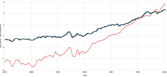
Logarithms of the yearly dividend data and the three types of sampled stock price data are presented in Figure 1.9 The different types of sampling of the stock prices appear to make very little difference to the properties of the resulting series, while both variables display upward trends over the sample period. Ghysels and Miller (2015) use demeaned data in their cointegration analysis, arguing that any trends in the series should be the same and the drifts will cancel out. This does not seem to be supported by inspection of Figure 1 in which the slopes appear to be significantly different. They also argue that cointegration is not to be expected owing to the increasing proportion of tech companies, many of which do not pay dividends, since the 1990’s leading to a structural break or a breakdown in the relationship between these variables. In the analysis below we use both demeaned and detrended data and proceed on the basis of cointegration. We also examine the residual plots from the cointegrating regressions for any obvious evidence of nonstationarity.
We begin with the demeaned data, which are depicted in Figure 2. The upward trends clearly remain in the demeaned series, as would be expected. The dividend data lie below the price data in the first half of the sample and then rise and remain above the prices in the second half of the sample, the cross-over point being around 1950. We compute OLS as well as the spectral and augmented spectral regression estimators using m = [Tδ] for δ={0.3,0.5,07} (the values that were used in the simulations), yieldingm={4,12,32}for T = 146. The underlying regression of interest is of the form
logPτ h=ClogDτ h+uτ h, τ = 1, . . . , N,
where P denotes stock price and D dividends. In view of unit roots in logP and logD, stationarity of the log price-dividend ratio, log(P/D), suggests that the cointegrating pa-rameter should be equal to unity. We therefore test H0:C = 1 against H1:C 6= 1 using
the Wald statistics proposed in section 3. Results using the demeaned data are presented in Table 3. As can be seen from Table 3, the estimates ofC are stable at around 0.52 with small standard errors, suggesting that the data are sufficiently informative to reject the hy-pothesis thatC = 1. Indeed, the Wald statistics are highly significant. The residuals from the cointegrating regression using the augmented spectral regression estimator withm = 4 and averaged price data (in which the estimated coefficient is 0.5251) are graphed in Figure 3. The residuals are reasonably stable although there is evidence of trending towards the end of the sample period.
A plot of the detrended data is given in Figure 4. Unlike the demeaned data there is much more variation in the series with multiple crossing points. The results obtained with the detrended data are given in Table 4. The OLS estimates of C are very similar to those obtained with the demeaned data but the spectral estimators are uniformly larger at roughly 0.57; the standard errors are also larger than those computed with the demeaned data. The Wald statistics are also lower than those with the demeaned data although all remain highly significant (the largest significance is obtained with the spectral estimator usingm= 4 with the end-of-period price data, although the value is only 0.001). Figure 5 plots the residuals from the cointegrating regression using the augmented spectral regression estimator with m= 4 and averaged price data (in which the estimated coefficient is 0.5727). The residuals
9To be consistent with the theory in section 2, the averaged stock price data are the yearly averages of
display the same pattern as those obtained with the detrended data.
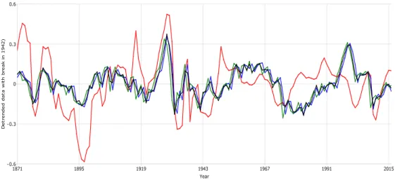
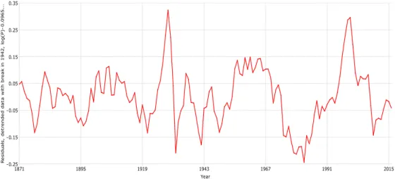
The detrended data in Figure 4 are suggestive of a possible trend break around the middle of the sample. Detrending the two sub-periods, 1871–1942 and 1943–2016, separately, yields the detrended data in Figure 6, in which there is no evidence of any remaining trends. Using the break-detrended data for estimation has a significant impact on the results, which are reported in Table 5. Estimates of C are much lower than those reported in Tables 3 and 4 and the standard errors are larger. The choice of m also has a greater impact on the spectral regression estimates than previously, ranging from roughly 0.10 withm= 4 to 0.22 withm= 12 and between 0.11 and 0.18 with m= 32. In all cases the null hypothesis C = 1 is convincingly rejected. The residuals from the cointegrating regression using the augmented spectral regression estimator with m= 4 and averaged price data (in which the estimated coefficient is 0.0965) are displayed in Figure 7. These residuals show slightly less dispersion than those reported earlier although there are a couple of noticeable spikes.
6. Concluding comments
This paper has proposed a model suitable for exploiting fully the information contained in mixed frequency and mixed sample data in the estimation of cointegrating vectors. The properties of easy-to-compute spectral regression estimators of the cointegrating parameters have been derived, these being in the form of theoretical asymptotic properties as well as simulated finite sample properties. The proposed estimators belong to the class of optimal cointegration estimators defined by Phillips (1991c) and Wald statistics based on these esti-mators have asymptotic chi-square distributions. The finite sample performance of a spectral regression estimator in an augmented mixed frequency model is particularly encouraging as it is capable of dramatically reducing the RMSE obtained in an entirely low frequency model to the levels comparable to an infeasible high frequency model. The size and power prop-erties of the associated Wald statistic are also good. An empirical example, to stock price and dividend data, was also provided to demonstrate the methods in practice.
The model analysed contains no deterministic components but it is a straightforward matter to deal with an intercept and time trend, for example. Demeaning and detrending the data by regression methods prior to the application of the frequency domain regression to estimate the cointegration parameters – such as is carried out in the empirical example – is a valid approach in which the limiting distributions are defined in terms of demeaned and detrended Brownian motion processes. Such an approach is valid because the cointegration parameters are assumed to be fixed, thereby avoiding the problems highlighted by Corbae, Ouliaris and Phillips (2002) in band limited spectral regression in models in which the pa-rameters are frequency-dependent. Alternatively the intercept and trend could be estimated as part of the spectral regression procedure. An assessment of the finite sample effects of these alternative approaches would constitute an interesting research exercise.
Appendix
Proofs of Lemmas and Theorems
Proof of Lemma 1. (a) We begin the derivation of the mixed frequency representation by selecting the firstn1 equations from (8) relating to y1t, which are given by
y1t=Cy2,t−1+v1t, t= 1, . . . , T. (35) The firstnS1 equations relating to yS1t are
y1St=CSSy2S,t−1+CSFy2F,t−1+vS1t, t= 1, . . . , T, (36) where v1t has been partitioned as v1t = v1St0, v1Ft0
0
. In view of Y2Ft being observed as an average of the unobservableyF
2tbetweent−1 andtit makes sense to aggregate this equation in the same way. As Y2Ft =k−1s(Lh)yF2t we apply the operatork−1s(Lh) to (36) to obtain (9) with ξS1t=k−1Pk−1
l=0 v1S,t−lh. The representation forY1Ft is obtained in the same way by applying the same filter to the lastnF
1 equations of (35), which are
y1Ft=CF Sy2S,t−1+CF FyF2,t−1+v1Ft, t= 1, . . . , T. (37) The result is (10) withξ1Ft=k−1Pk−1
l=0 v1F,t−lh. Finally, the stochastic trends forY2St andY2Ft are obtained by applying the same filter again, this time to (7), resulting in (11) and (12) withξ2St=k−1Pk−1
l=0 wS2,t−lh and ξF2t=k−1
Pk−1
l=0 wF2,t−lh.
(b) The objective in the feasible low frequency representation is to skip-sample the high fre-quency stock variables at integer values ofτ hand relate them to the observed low frequency flows. The equation fory1St is obtained from (36) as follows:
y1St = CSSy2S,t−1+CSFy2F,t−1+v1St
= CSSy2S,t−1+CSFY2F,t−1+v1St+CSF yF2,t−1−Y2F,t−1
= CSSy2S,t−1+CSFY2F,t−1+ζ1St,
whereζ1St=v1St+CSFδ2F,t−1 and δ2F,t−1 =y2F,t−1−Y2F,t−1 is I(0) using Lemma A1 withj= 0.
ForYF
1t a similar procedure can be carried out using (10): Y1Ft = CF SY2S,t−1+CF FY2F,t−1+ξ1Ft
= CF Sy2S,t−1+CF FY2F,t−1+ξ1Ft+CF S Y2S,t−1−yS2,t−1
= CF Sy2S,t−1+CF FY2F,t−1+ζ1Ft,
where ζ1Ft =ξF1t−CF Sδ2S,t−1 is I(0) using Lemma A1. Finally, the stochastic trends fory2St come directly from the first nS2 equations of (7), so thatζ2St =wS2t, while those for Y2Ft are simply (12), so thatζ2Ft=ξF2t. 2
ut as follows: 1 √ T [T r] X t=1 ξt=G(Lh)s(Lh)√1 T [T r] X t=1 ut.
The task is then to relate the partial sums involving fractions ofTto the FCLT in Assumption 1 which deals with the high frequency process and partial sums involving a fraction of N. Following the proof of Lemma 1 of Miller (2016) we can write
[N r] X τ=1 uτ h = [T r] X t=1 k−1 X l=0 ut−lh+ [N r] X l=[T r]/h+1 ulh = s(Lh) [T r] X t=1 ut+ [N r] X l=[T r]/h+1 ulh.
from which we obtain
s(Lh)√1 T [T r] X t=1 ut = √1 T [N r] X τ=1 uτ h−√1 T [N r] X l=[T r]/h+1 ulh = √1 T [N r] X τ=1 uτ h+op(1),
the last quantity being asymptotically negligible owing to the summation being over a finite interval and hence will converge to zero, as shown in Miller (2016). Now, the elements of G(z) are polynomials of order no greater than k−1 so we can use Lemma 2.1 of Phillips and Solo (1992) to write
G(z) =G(1)−(1−z) ˜G(z)
where the elements of ˜G(z) are polynomials of order no greater than k−2. We can then write, usingT =hN, 1 √ T [T r] X t=1 ξt = √1 hG(1) 1 √ N [N r] X τ=1 uτ h− 1 √ h ˜ G(Lh)√1 N [N r] X τ=1 ∆huτ h+op(1) = √1 hG(1) 1 √ N [N r] X τ=1 uτ h+op(1) because 1 √ N [N r] X τ=1 ∆huτ h = 1 √ N u[N r]h−u0 =op(1). It follows that, asT → ∞, 1 √ T [T r] X t=1 ξt→d B(r)
whereB(r) = (1/√h)G(1)Bu(r) is a Brownian motion process with covariance matrix Ω as defined in the Lemma. 2
Proof of Lemma 3. Let Mu(z) = P∞l=−∞Γu,lhzlh denote the autocovariance generating function (AGF) ofuτ h. Then, from Hamilton (1994, p.268) the AGF ofξt,measured in high
frequency time units, is given by
MH(z) =G(zh)s(zh)Mu(z)s(z−h)G(z−h)0 =
∞ X
l=−∞
Γξ,lhzlh,
where Γξ,lh = E(ξtξt0−lh) is the high frequency autocovariance matrix at lag lh for ξt at the high frequency. To convert this to the low frequency time units we take integer values (settingm=lh) to give M(z) = ∞ X m=−∞ Γξ,mzm.
In case where the limits inMH(z) are finite, such as for a finite-order moving average, an ap-propriate adjustment needs to be made to the limits inM(z) i.e. ifMH(z) =PK
l=−KΓξ,lhzlh then M(z) = P[mKh=−[] Kh]Γξ,mzm. The aim is to first relate Γξ,lh to Γu,lh. The product s(z)s(z−1) is a two-sided scalar polynomial of orderk−1:
s(z)s(z−1) = k−1 X l=0 zl k−1 X m=0 z−m = k−1 X l=−(k−1) s1lzl
where thes1l coefficients are implicitly defined. Next, let
Γu,lh =
Γ11u,lh Γ12u,lh Γ21u,lh Γ22u,lh
!
.
Then, from the form ofG(z) in Lemma A2, we find that
G(z)Mu(z)G(z−1)0 =h2 ∞ X l=−∞ Clh11 Clh12 Clh21 Clh22 ! , where
Clh11 = Γ11u,lh+s(z)CΓ21u,lh+s(z−1)Γ12u,lhC0+s(z)s(z−1)CΓ22u,lhC0, Clh12 = s(z−1)Γ12u,lh+s(z)s(z−1)CΓ22u,lh,
Clh21 = s(z)Γ21u,lh+s(z)s(z−1)Γ22u,lhC0, Clh22 = s(z)s(z−1)Γ22u,lh.
s(z)s(z−1) itself, s(z)2s(z−1) = k−1 X m=0 zm k−1 X l=−(k−1) s1lz−l= 2k−2 X l=−(k−1) s2lzl, s(z)s(z−1)2 = k−1 X l=−(k−1) s1lzl k−1 X m=0 z−m= k−1 X l=−(2k−2) s3lzl, s(z)2s(z−1)2 = k−1 X l=−(k−1) s1lzl k−1 X m=−(k−1) s1lz−m= 2k−2 X l=−(2k−2) s4lzl,
where the coefficients are again implicitly defined. Hence each summand of interest, Γu,lh, is multiplied by a finite-order scalar polynomial inzh of order 2k−2 at most. We therefore need to consider quantities of the form (withp= 2k−2)
p X m=−p amzmh ∞ X l=−∞ Γu,lhzlh= ∞ X l=−∞ p X m=−p amΓu,lh−mh ! zlh,
which implies that Γξ,lh=Ppm=−pamΓu,lh−mh. Taking integer values of lhwe obtain T X l=−T |l|kΓξ,lk = T X l=−T |l| p X m=−p amΓu,lh−mh ≤ p X m=−p |am| T X l=−T |l|kΓu,lh−mhk=O(T1/2)
which implies the required result asp is finite and independent ofT. 2
Proof of Theorem 1. (a) We begin by noting that we can write ˆ f22(0) = 1 2m+ 1 m X j=−m I22(λj) = 1 2m+ 1 m X j=−m 1 2π T−1 X k=−T+1 ˆ Γ22,ke−ikλj ! = 1 2π(2m+ 1) T−1 X k=−T+1 ˆ Γ22,kwk
wherewk=Pmj=−me−ikλj and
ˆ Γ22,k = 1 T T X t=k+2 Y2,t−1Y20,t−1−k, k≥0, 1 T T+k X t=2 Y2,t−1Y20,t−1−k, k <0.
We are then led to consider 2m+ 1 T2 fˆ22(0) = 1 2πT T−1 X k=−T+1 1 TΓˆ22,k wk d → 1 2π Z 1 0 B2B02× lim T→∞ 1 T T−1 X k=−T+1 wk = 1 π Z 1 0 B2B20
using Lemma A3(a) and as the limit involving the sum ofwkis equal to 2; see Lemma A4(a). (b) Proceeding in a similar way as in part (a) we find that
ˆ fξ2(0) = 1 2m+ 1 m X j=−m Iξ2(λj) = 1 2π(2m+ 1) T−1 X k=−T+1 ˆ Γξ2,kwk
wherewk is as previously defined and
ˆ Γξ2,k= 1 T T X t=k+2 ξtY20,t−1−k, k≥0, 1 T T+k X t=2 ξtY20,t−1−k, k <0.
We are then led to consider 2m+ 1 T ˆ fξ2(0) = 1 2πT T−1 X k=−T+1 1 TΓˆξ2,k wk d → 1 2π Z 1 0 dBB20 × lim T→∞ 1 T T−1 X k=−T+1 wk+ lim T→∞ 1 2πT T−1 X k=−T+1 S2,k+1wk = 1 π Z 1 0 dBB02+ lim T→∞ 1 2πT T−1 X k=−T+1 S2,k+1wk
using Lemma A3(b) and Lemma A4(a) and whereS2,k =P∞l=kΓξ2,l. Using summation-by-parts the second term can be written
1 T T−1 X k=−T+1 S2,k+1wk = S2,T 1 T T−1 X k=−T+1 wk ! + T−2 X k=−T+1 1 T k X l=−T+1 wl ! (S2,k+1−S2,k+2) = S2,T 1 T T−1 X k=−T+1 wk ! + T−2 X k=−T+1 1 T k X l=−T+1 wl ! Γξ2,k+1
becauseS2,k+1−S2,k+2= Γξ2,k+1. NowS2,T →0 as T → ∞ while, from Lemma A4(a), 1 T T−1 X k=−T+1 wk→2,
hence the first term converges to zero. As for the second term we have, from Lemma A4(b), 1 T k X l=−T+1 wl= 1 +O m T
for allk, and so we deduce that, under Assumption 2,
lim T→∞ 1 2πT T−1 X k=−T+1 S2,k+1wk = 1 2π ∞ X k=−∞ Γξ2,k as required.
(c) We begin by using the decomposition ˆ fξˆξˆ(0)−fξξ(0) = ˆ fξˆξˆ(0)−fˆξξ(0) +fˆξξ(0)−fξξ(0)
and then proceed to show that each of the two terms in parentheses isop(1). Note that
ˆ fξˆξˆ(0) = 1 2m+ 1 m X j=−m wξˆ(λj)wξˆ(λj)∗
and that ˆξt=Y0t−JCYˆ 2,t−1where ˆCis an initial estimator ofCsuch thatT( ˆC−C) =Op(1). Substituting forY0t we obtain ˆξt=ξt−J( ˆC−C)Y2,t−1 which implies that
wξˆ(λj) =wξ(λj)−J( ˆC−C)w2(λj).
It then follows that
Iξˆξˆ(λj) = wξˆ(λj)wξˆ(λj)∗ = wξ(λj)−J( ˆC−C)w2(λj) wξ(λj)−J( ˆC−C)w2(λj) ∗ = Iξξ(λj) +J( ˆC−C)I22(λj)( ˆC−C)0J0−J( ˆC−C)I2ξ(λj)−Iξ2(λj)( ˆC−C)0J0
and so the quantity of interest is
ˆ fξˆξˆ(0)−fˆξξ(0) = 1 2m+ 1 m X j=−m Iξˆξˆ(λj)−Iξξ(λj) = J( ˆC−C) ˆf22(0)( ˆC−C)0J0−J( ˆC−C) ˆf2ξ(0)−fˆξ2(0)( ˆC−C)0J0.
Using the stochastic orders of magnitude already established we obtain (2m+ 1)fˆξˆξˆ(0)−fˆξξ(0) = J T( ˆC−C)2m+ 1 T2 fˆ22(0)T( ˆC−C) 0J0 −J T( ˆC−C)2m+ 1 T ˆ f2ξ(0)− 2m+ 1 T ˆ fξ2(0)T( ˆC−C)0J0 = Op(1)
and so ˆfξˆξˆ(0)−fˆξξ(0) =Op(1/m) =op(1) under Assumption 2. The second term of interest can be shown to be op(1) if Assumption 3 holds in addition to Assumptions 1 and 2 as Lemma 3 can be used to control the rate of growth of the autocovariances ofξt. This second term is a consistency result for the infeasible smoothed periodogram estimator based on the unobservable ξt and follows, for example, from results in Hannan (1970) and Fuller (1996). 2
Proof of Theorem 2. From Theorem 1(c) we can replace ˆfξˆξˆ(0) with fξξ(0) and so, from (24), we are led to consider
T( ˆC0−C) = J0fξξ(0)−1J −1 J0fξξ(0)−1 2m+ 1 T fˆξ2(0) 2m+ 1 T2 fˆ22(0) −1 +op(1) d → J0fξξ(0)−1J −1 J0fξξ(0)−1 1 π Z 1 0 dBB20 + 1 2πΩ2 1 π Z 1 0 B2B20 −1 = J0fξξ(0)−1J−1J0fξξ(0)−1 Z 1 0 dBB20 Z 1 0 B2B20 −1 +1 2 J 0 fξξ(0)−1J−1J0fξξ(0)−1Ω2 Z 1 0 B2B20 −1 .
Using the definitions 2πfξξ(0) = Ω and Ω11.2= Ω11−Ω12Ω−122Ω21 it can be shown that
J0fξξ(0)−1J = 2πΩ−111.2 and J 0 fξξ(0)−1 = 2π Ω−111.2 :−Ω −1 11.2Ω12Ω −1 22 , results which imply that
J0fξξ(0)−1J−1J0fξξ(0)−1 = In1 :−Ω12Ω
−1 22
. Hence the first term in the limiting distribution can be written
Z 1 0 dB1.2B02 Z 1 0 B2B20 −1 whereB1.2 = In1 :−Ω12Ω −1 22
B =B1−Ω12Ω−122B2. For the second term we begin by noting
that Ω2= Ω 0n1×n2 In2 ! = 0
and, hence, it follows that J0Ω−1Ω2 = (In1 : 0n1×n2)Ω −1Ω 0n1×n2 In2 ! = 0.
This demonstrates that the second term is zero and the limiting distribution is defined as in the Theorem. 2
Proof of Theorem 3. We begin withW0 and note that the limiting distribution of ˆγ0 has
the representation T(ˆγ0−γ) d → " Z 1 0 B2B20 −1 ⊗In1 # Z 1 0 (B2⊗dB1.2). LetM22= R1 0 B2B 0
2. Then, from the proof of Lemma 5.1 in Park and Phillips (1988), Z 1 0 (B2⊗dB1.2) B2 ∼N(0, M22⊗Ω11.2)
in view ofB2 and B1.2 being independent. It then follows that the limiting distribution of
T(ˆγ0−γ),conditional onB2, isN(0, M22−1⊗Ω11.2). Now consider
r(ˆγ0) =r(γ) +R(¯γ)(ˆγ0−γ),
where the elements of ¯γ lie on the line segment between ˆγ0and γ. UnderH0,r(γ) = 0 while
the consistency of ˆγ0 ensures thatR(¯γ)
p
→R(γ) =R0. Then it follows that
T r(ˆγ0) =R(¯γ)T(ˆγ0−γ) d →R0 " Z 1 0 B2B20 −1 ⊗In1 # Z 1 0 (B2⊗dB1.2)R00.
This limiting distribution, conditional on B2, is N(0, R0QR00) where Q = M −1
22 ⊗Ω11.2.
Theorem 1 implies that
2m+ 1 2T2 Vˆ0
d →Q−1 and hence we are led to consider
W0=T r(ˆγ0)0 " R(ˆγ0) 2m+ 1 2T2 Vˆ0 −1 R(ˆγ0)0 #−1 T r(ˆγ0).
The limiting distribution of this quantity, conditional on B2, involves a quadratic form
in N(0, R0QR00) random variables weighted by the matrix (R0QR00)−1, and hence is χ2q. But because this does not depend on B2 it is also the unconditional distribution. Similar
arguments apply toW0A. 2
Proof of Proposition 1. (a) The proof follows that of Lemma 2 based on 1 √ T [T r] X t=1 ζt=Gζ(Lh)s(Lh) 1 √ T [T r] X t=1 ut.