Universidade de São Paulo
2015-02
A projection pursuit framework for supervised
dimension reduction of high dimensional small
sample datasets
Neurocomputing, Amsterdam, v. 149, p. 767-776, Feb. 2015
http://www.producao.usp.br/handle/BDPI/50247
Downloaded from: Biblioteca Digital da Produção Intelectual - BDPI, Universidade de São Paulo
Biblioteca Digital da Produção Intelectual - BDPI
A Projection Pursuit framework for supervised dimension reduction
of high dimensional small sample datasets
Soledad Espezua
a,n, Edwin Villanueva
a, Carlos D. Maciel
b, André Carvalho
a aDepartment of Computer Science, ICMC - USP, University of São Paulo, Brazil
bDepartment of Electrical Engineering, São Carlos School of Engineering, University of São Paulo, Brazil
a r t i c l e i n f o
Article history:
Received 6 June 2013 Received in revised form 2 June 2014
Accepted 28 July 2014
Communicated by Shiguang Shan Available online 12 August 2014
Keywords: Projection Pursuit Classification Gene expression Dimension reduction
a b s t r a c t
The analysis and interpretation of datasets with large number of features and few examples has remained as a challenging problem in the scientific community, owing to the difficulties associated with the curse-of-the-dimensionality phenomenon. Projection Pursuit (PP) has shown promise in circum-venting this phenomenon by searching low-dimensional projections of the data where meaningful structures are exposed. However, PP faces computational difficulties in dealing with datasets containing thousands of features (typical in genomics and proteomics) due to the vast quantity of parameters to optimize. In this paper we describe and evaluate a PP framework aimed at relieving such difficulties and thus ease the construction of classifier systems. The framework is a two-stage approach, where thefirst stage performs a rapid compaction of the data and the second stage implements the PP search using an improved version of the SPP method (Guo et al., 2000,[32]). In an experimental evaluation with eight public microarray datasets we showed that some configurations of the proposed framework can clearly overtake the performance of eight well-established dimension reduction methods in their ability to pack more discriminatory information into fewer dimensions.
&2014 Elsevier B.V. All rights reserved.
1. Introduction
In the last few decades we have witnessed a rapid development and refinement of data acquisition technologies in several science and industrial areas[1]. This has led to the emergence of high-throughput technologies that are capable of generating datasets with the number of features (p) far greater than the number of examples (n), the so-calledlarge p small ndatasets. A representa-tive example of these technological developments is the micro-array technology[2], which has made possible the measurement of expression levels of thousands of genes in a relatively rapid and economic way, leading to significant advances in the under-standing of severe diseases, like cancer, and raising hopes on possible cures[3,4].
Though the collection oflarge p small ndatasets is nowadays a common practice in manyfields, their analysis and interpretation is still a challenging task[5,6,1]. This difficulty is mainly originated by the so-called“curse of dimensionality”phenomenon, inherent in such a kind of data[7]. This phenomenon states that as the dimensionality increases, the corresponding space becomes emp-tier and the data points tend to be equidistant. This generates
detrimental impacts in most machine-learning and pattern-recog-nition methods (including model-estimation instability, model over fitting and local convergence), compromising the general-ization performance and reliability of such methods[5,6].
A common approach to circumvent the curse of dimensionality is by reducing it [6]. Two kinds of methods exist for this task: feature selection (FS) [8,9] and feature extraction (FE) [10,11]. The former methods try tofind small subsets of original features that are relevant to the intended analysis. The latter methods reduce the dimensionality by building new features from combi-nations (linear or nonlinear) of the original features. FS has the benefit of keeping the original feature meaning, facilitating the interpretability by the domain expert [9]. However, it has been said[12] that FE is preferable over FS when thefinal goal is an accurate system for classifying new examples and interpretability is not as important. This is because FE is not tied to the original feature space, providing greater chances of finding more useful representations for the desired task[12].
Projection pursuit (PP) [13,14]is a FE method that has been successfully applied in several domains for both supervised and unsupervised analyses (e.g. [15–18]). PP seeks low-dimensional linear projections of the data that expose interesting aspects of them. To this end, a measure of“interestingness”is employed, which is known as projection pursuit index (PP index). A key advantage of PP is itsflexibility tofit different pattern recognition tasks, depending on the PP index used. For example, PP can be Contents lists available atScienceDirect
journal homepage:www.elsevier.com/locate/neucom
Neurocomputing
http://dx.doi.org/10.1016/j.neucom.2014.07.057
0925-2312/&2014 Elsevier B.V. All rights reserved.
nCorresponding author. Tel.:þ55 16 34132126.
E-mail addresses:[email protected](S. Espezua),[email protected](E. Villanueva),
[email protected](C.D. Maciel),[email protected](A. Carvalho).
used to perform clustering analysis[19,20], classification[21–24], regression analysis[25]and density estimation[26](some reviews of PP indexes can be found in [21,27,28]). Another advantage of PP is its out-of-sample mapping capability, that is, the possibi-lity to map new examples in the projection space after the con-struction of it.
Despite the aforementioned advantages, the literature shows a limited use of PP inlarge p small ndatasets, like those generated by microarray technology. This may be due to the high computational difficulty in finding optimal projection spaces for such cases. For instance, the projection of a dataset with p¼10k features (a realistic number in microarray datasets) onto a target space of dimension m¼3 will require the optimization of a projection matrix ofpm¼ 30k elements. Evidently, the problem worsens as p or m increase. Traditional PP optimizers based on the gradients or Newton methods[29–31,19]are usually inadequate for such a kind of data due to the vastness of possible projections and, thus, the high susceptibility to find poor local optima [14]. More global PP optimizers were described recently, including genetic algorithms (GA)[32,33], simulating annealing (SA) [21], random scan sampling (RSSA)[34]and particle swarm optimiza-tion (PSO)[35]. However, none of these works have been directly applied in dimensionalities as high as those found in microarray data, which shows the difficulty of applying PP in such scenarios. In this paper we present a framework to facilitate the applic-ability of PP onlarge p small ndatasets with the aim of classifi ca-tion tasks. The framework is formed by two main stages (Fig. 1): a compaction stage and a PP optimization stage. Thefirst stage is devised to rapidly transform the original data into a less sparse representation. The second stage is the PP part, which is respon-sible tofind optimal projections taking the compacted representa-tion as input.
For the compaction stage we use three well-known techniques: PCA, Whitening and Partial Least Squares. For the PP stage, we adopt the Sequential Projection Pursuit (SPP) approach [32]
coupled with the GA optimizer (PPGA) we described recently
[33], in which a specialized crossover operator showed excelling search capabilities. An experimental study is presented over eight public microarray datasets. The evaluation systematically tested several configurations of the framework, including variations of the compaction method, the PP index function and the target dimensionality. We used the predictive accuracy of two popular classification methods (LDA and 3NN) in order to assess the quality of the tested configurations. We also compare the framework against eight well-established dimension reduction methods, including FE and FS methods.
The paper is organized as follows.Section 2introduces some important concepts of PP, SPP, PP optimization and PP indexes used in the paper.Section 3describes the proposed framework.
Section 4 presents the experimental evaluation, including the experimental setup, results and corresponding discussion. Finally, our conclusions are presented inSection 5.
2. Projection pursuit
The projection pursuit (PP) concept was formally introduced in the paper of Friedman and Tukey[13], although the seminal ideas were originally posed by Kruskal[36]. To describe the PP concept we assume that we have a data matrix Xof npdimensions, wherenis the number of data examples or observations andpis
the number of attributes or variables. PP can be defined as the constrained optimization problem in(1), where the aim is to seek am-dimensional projection spaceðmopÞ(defined by the bases–
columns–ofA¼ ½a1;…;amARpm) such that the projected data
points in that space maximize a pre-defined objective functionI, called the projection pursuit index. This function measures the degree of interestingness of the projected data. The constraint of orthonormality inAis necessary to ensure that each dimension in the target space shows different aspects of the data:
An¼arg max
A
fIðXAÞg
s:tATA¼I: ð1Þ
2.1. Sequential projection pursuit
Sequential projection pursuit (SPP)[32]solves the PP problem in (1) by decomposing it into a sequence of m optimization problems, each computing one base inA.
The first base, a1, is obtained by searching a p-dimensional
unit-length vector where the projected dataXa1 maximizes the
one-dimension PP indexI. Oncea1is found, SPP tries to remove
all the information captured in that direction from the original data in order to avoid finding the same projection direction in subsequent iterations. For this task, the original SPP uses a
“structure removal”procedure[14], which“Gaussianize”the data in the found direction, as follows:X¼XXa1aT1. The next basea2
is sought taking the updatedX(also calledresidual data) as input data, subject to the constraint thata2 is orthogonal to a1. The
process is iteratively repeated until allmbases are obtained.
2.2. PP optimization
A key component in PP is the optimization process. Early approaches in this respect were based on the gradient techniques
[30,29]and Newton–Raphson[31,37,14,13], where the projections are performed in at most three dimensions for visual exploratory tasks, the so-called exploratory projection pursuit (EPP). Further developments focused on developing more global methods for PP optimization, such as random search[38,39,29], genetic algorithm (GA)[32], random scan sampling algorithm (RSSA)[34], simulated annealing (SA)[21], particle swarm optimization (PSO) [35]and tribes [40]. In a previous work [33] we describe PPGA, a GA optimizer with a specialized crossover operator that often showed to find solutions better than those found by PSO, RSSA, and SA when used inside the SPP framework, reason why it is adopted for the present work.
Another important aspect in optimizing PP is how to ensure that each resulting dimension is associated with a different and complementary aspect of the data. Many PP methodologies, including SPP, address this task by using the“structure removal”
procedure. However, it has been observed[41,38]that the succes-sive application of this procedure (as done in the original SPP) may lead to data distortions, implying that an optimum found in residual data may not be longer related to any relevant aspect of the original data. Recently, Zhang and Chan [41,28] proposed an alternative approach to structure removal, which uses the
orthogonal complement spaceconcept.1In those works, the residual
data is obtained projecting the current data onto the orthogonal complement of the found projection vector, which avoid data distortions and also ensures orthogonality of the projection bases.
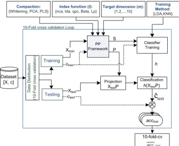
Fig. 1.Framework WSPP.
1
The orthogonal complement of one vectorxARnis the vector spacey, all of
which are orthogonal tox. Therefore, such space can be expanded byn1 vector basis. That is, the orthogonal space of a vector x n-dimensional is always dimensional sizen1.
2.3. Projection pursuit indices
The choice of the PP index is very important, since it defines what is“interesting”in the data. A great deal of research in the PP community has been centered on the construction of meaningful PP indexes for different purposes. It is possible tofind PP indexes for clustering analysis[42,19,38,39,43,30,13], for supervised ana-lysis[44,45,21,5] and for regression analysis [46,47]. Given that this paper is targeted to supervised analysis, we briefly describe some relevant supervised PP indexes included in the experimental evaluation of the paper. To facilitate the description we consider that each example xiAX has associated a class label ciAC¼ f1;…;cmaxg.
Index Bhattacharya(Bat): It is based on the Bhattacharya distance
between classes and uses statistics of first and second orders. The Bhattacharya index for 1D projection space2 is defined as[28,5] IBat¼min i;jAC 1 4 ð
μ
iμ
jÞ2σ
iþσ
j þ1 2logσ
iþσ
j 2pffiffiffiffiffiffiffiffiffiσ
iσ
j ( ) ; ð2Þwhere
μ
iandσ
idenote respectively the mean and thevariance of the projected examplesXaof classi.
Index quality projected clusters(qpc): This index favors projections
that allows us tofind compact pure clusters of vectors separated from other clusters[24,44]. The qpc index for 1D projection space is defined as
Iqpc¼ ∑
n i;j¼1
α
i;jGððxixjÞaÞ; ð3Þ
where
α
i;j40 if the examples xiand xj belong to thesame class (ci¼cj), in other case
α
i;jo0. Function Gð:Þshould be localized with maximum forx¼0 (e.g. Gaus-sian function).
Index Fisher linear discriminant analysis (lda): This index was
adapted from the classical LDA method[27,21]and favors linear projections with greater separation between classes (in the sense of least squares) and lower dispersion intra-classes. Eq. (4) shows the formula for the index calculation[45]:
Ilda¼1
jATWAj
jATðWþBÞAj; ð4Þ
whereBis the between-class scatter matrix andWis the within-class scatter matrix.
Index neighborhood components analysis (nca): This index was
not proposed as such but as a cost function in the nca method[48]. It has successfully used in several applica-tions (e.g. [49–51]), reason why it is included in the present study. The cost function is derived from a stochastic neighbor assignment scheme and is propor-tional to the expected number of points correctly classi-fied under that scheme:
Inca¼∑ n i jA∑Ωi
pij; ð5Þ
where
Ω
idenote the set of examples in the same class as ibyΩ
i¼ fjjci¼cjg;pii¼0 andpij¼expðJxiAxjAJ2Þ= ∑kaiexpðJxiAxkAJ2Þis the probability of exampleiselecting example j as its neighbor and inheriting its class label.
Index locality preserving(Lp): This is an unsupervised index based
on the Locality Preserving Projections (LPP) method[52]. This index favors projections that concentrate the neigh-boring data examples together. We define here the Lp index(6)as the inverse of the original LPP criterion (this was defined for minimization):
ILp¼1=ðATXLAÞ; ð6Þ
where L is a Laplacian matrix of the k-neighborhood graph (graph obtained by linking the k nearest neighbors to each example).
3. A PP framework for supervised dimension reduction of large p small n data
We detail here the proposed framework to ease the applic-ability of PP in largepsmallndata.Fig. 2shows the structure of this framework. Two stages compose this: the first stage imple-ments a fast procedure to compact the data into an intermediate-dimensional representation (in the order ofn). The second stage is a PP procedure over the compacted data, which implements an improved version of the SPP scheme. Next, we describe each framework component:
3.1. Compaction stage
The goal of compaction stage is to reduce the high p -dimen-sional space X to a less sparse q-dimensional space W, where the original information is preserved as much as possible. In this paper we tested the following methods for this purpose, based on their popularity, availability of implementations and ease of computation:
The whitening transform(Whiten)[53]: It is also calledsphering,and is a popular data transformation that produces uncorre-lated and normalized attributes. The effects of whitening on largepsmallndata were recently studied by Deng et al.[54], finding that the whitened data points lie at the vertices of a regular (n1)-dimensional simplex. This means that any distance-based method fails to work in the full whitened data, since all data points are equidistant. However, the authors also show that by pruning out some irrelevant attributes (those associated with the lowest singular values) of the transformed data, it is possible to produce highly informative data for subsequent analysis. In a related study, Vicente et al.[53]found that the most influential part on the performance of ICA is the whitened transformation. Various other authors pointed the feasibility of whitening as a pre-processing step in microarray data analysis [55–61]. Whitening is performed via singular value decomposition (SVD) on the centered3data matrixX:
X¼UDVT; ð7Þ
whereUARnn
is the matrix of eigenvectors ofXTX;DARnn
is a diagonal matrix containing the singular values of XTX
(ordered in descending order); VARpn
is the matrix of eigenvectors ofXXT. The whitened dataWARnq
is the matrix formed by thefirst qcolumns ofU. This can be expressed in terms of the input data asW¼XR, whereR¼V~D~1ARpq
is the whitening transformation matrix (also used to get thefinal projection matrix) andV~ARpqandD~ARqqare obtained by
2
In 1D projection spaces we useainstead ofAto denote the projection base. 3
Data resulting of subtracting the column-mean from the original data.
taking the first q columns of V and the upper left q q
submatrix ofD, respectively.
Principal component analysis (PCA) [62]: It is a well-knownmethod of dimension reduction, which is used to construct a set of orthogonal components by maximizing the variance of the linear combinations of the original predictors. Similar to Whitening, the sequence of principal components (PCs) is the reduced matrixV~ARpq
, which can also be expressed in terms of the input data asW¼XRARnq
, whereR¼V~ is the PCA transformation matrix.
In both PCA and Whitening the transformation matrix R
has the constraintsRTR¼I in order to ensure orthogonality. Geometrically, the PCA transformation (without pruning) represents a rotation of the original coordinate system such that the new axes are the directions of maximum variability in the original data [63]. In Whitening transformation (without pruning) the data points lie at the vertices of a regular (n 1)-dimensional simplex with all data points equidistant from each other[55].
Partial least squares (Pls): Pls is a wide class of supervisedmethods used for modeling relations between sets of observed variables by means of latent variables (also called the latent components). It has been defined for regression analysis, classification and dimension reduction[64]. Pls can be formu-lated as an optimization problem that aims to find a set of optimal weights vectors ri (i¼1,…,q) to maximize the
covar-iance between the response variable Y and the predictor variablesX, it can be defined as[63]
ri¼arg maxfCovðW;YÞg;
s:tWTW¼I ð8Þ
whereW¼XRARnq
represents the nobservations by theq
Pls components. The maximum number of componentsqis at most the rank of X. At each step i (i¼1,…,q), the vector
riAR¼ ½r1;…;rqis estimated by regression in such a way that
the Pls component,wiAW¼ ½w1;…;wq, has maximal example
covariance with the response variable Y, subject to being
uncorrelated with all previously constructed components. When Pls is used for classification problems, the vector of class label associated atXcan be expressed in terms of a response data matrix: YARnc dividing the number of class label in c
columns, being each column a binary vector with 1 in the associated class label and 0 in other case.
The technique is something of a cross between multiple linear regression and PCA. As a result, the Pls components are uncorrelated and ranked in the decreasing order and can be derived from[64]:
X¼WRTþerrorX; ð9Þ
Y¼WSTþerrorY; ð10Þ
whereRARpqare the matrix of predictors loading vectors (or weights) used for constructing the wi Pls components, S¼ ½s1;…;sqARcqare the response loading matrix.
We use the MATLABs (R2009b) Statistics Toolbox for the implementation of the previous compaction methods. They return the complete set of components along with the variance explained by each component. In all compaction methods we setqas the minimal number offirst components in which the cumulative sum of the respective variances is over 95% of the total sum of variances. This number was experimentally verified to conserve most discriminant information and, at the same time, reduces significantly the input dimension for the PP stage.
3.2. PP stage
This stage is responsible for the projection search over the compacted data. We follow the SPP approach in which the projection bases are obtained one-by-one in an iterative loop. Our current implementation of SPP replaces/modifies some com-ponents of the original SPP in order to improve performance. These components are described as follows:
Initial population: This component is new in SPP and isintended to improve the convergence time andfitness of the subsequent PP optimization. The recentCandidate Projection Set
(CPS) method [65] is used for that purpose, which obtains candidate projection bases using class boundary information. In the experiments, the size (w) of the initial population is set as w¼3q, formed by 50% of individuals from CPS and 50% created randomly.
Projection pursuit genetic algorithm(PPGA): This is the adoptedPP optimizer, taken from our previous work [33]. Unlike the original GA optimizer, which uses binary encoding and cano-nical operators, PPGA uses a real encoding and a specialized crossover operator (called the Inner-outer Hypercone cross-over). It was showed that this operator provides a good search capability for PP optimization in high dimensionalities [33]. At each generation, an offspring population is created with crossover. Mutation is not used in PPGA, since the crossover operator has high randomness and mutation showed to slow the convergence without any apparent improvement of the results. For mating selection we use tournament selection with tournament size equal to 3, a value that was adequate in the experimentation. The population for the next generation is formed by taking the best windividuals of the joint offspring and current population. PPGA ends when the difference in meanfitness between two successive generations falls within a given precision
Δ
or a maximum number of generationsg is achieved. In the experiments we useΔ
¼1e4andg¼300. Deflation/Inflation: These procedures implement an efficientway to ensure orthogonality of the projection bases and, thus,
to capture distinct and complementary aspect of the data. The original structure removal procedure of SPP is replaced by these procedures, which are based on the work of Rodriguez-Martinez et al.[28]. Deflation prepares the search space for the next iteration and is executed after PPGA completion (except when the required number of bases is attained, in which case the loop is halted). Specifically at iterationi, PPGA finds the basis bi from residual data matrix Zi ðnqiþ1Þ (at first
iteration, the residual data is the original whitened data Y). Deflation then usesbi to compute the set of basisQ
ðqiþ1;qiÞ i
that defines the orthogonal complement of bi. Then, the
current residual data are projected onto that space to get the residual data for the next iteration:Ziþ1¼ZiQi. Note that after
each deflation the dimension of the residual data decreases one unit, which means that the difficulty infinding bases decreases with the advance of the process (an advantage over the original structure removal procedure, which maintains a uniform diffi -culty along iterations). The inflation process is performed once all m bases are obtained. As each base bi is defined for its
corresponding residual data (of different dimensions), it is necessary to put all the bases in the original (compacted) space. Inflation, thus, constructs the projection matrix A
computing each baseai (iZ2) by multiplying all matricesQj,
for alljoi, and then the resulting matrix withbi (operation
known as base inflation).
Finally, once the PP stage ends and the projection matrixAis returned, the overall projection matrixPthat maps the input data
Xto the target space is computed, thusPpm¼RA.
4. Experimental evaluation
This section presents the experimental evaluation conducted over the proposed framework in order to determine its suitability in classification tasks of largepsmallndata.
4.1. Experimental setup
Eight public microarray datasets were used in the evaluation (Table 1). Fifteen configurations of the framework were evaluated, corresponding to all combinations of the compaction methods (Section 3.1) with thefive PP indexes ofSection 2.3. As evaluation metrics, we used the predictive accuracies of two popular classi-fication methods: Linear Discriminant Analysis (LDA) [74] and
K-Nearest Neighborhood (K-NN) (withk¼3)[75]over the reduced data resulting of each configuration. These methods were chosen by their popularity, simplicity, speed and few parameters to set up. Also, they are deterministic (with the same training data we get the same classifier), which means that the final classification results are only affected by the quality of the projections. The implementations used for LDA and K-NN algorithms were those available in the MatlabBioinformatics toolbox[76]. We additionally
included in the evaluation eight popular dimension reduction methods: Locally Linear Embedding (LLE) [77], Neighborhood components analysis (NCA)[48], Partial Least Squares (Pls) [64], Sliced Inverse Regression (SIR)[78], the three compaction meth-ods used in a standalone way, and two well-known feature selection methods (T-test Modified (T-testM) [79] and ReliefF
[80]). We used the following implementations for these methods: DRtoolbox [81]for LLE and NCA, Weka implementation[82] for ReliefF, Zhou's implementation[79]for T-testM, Matlab Statistics Toolbox for Pls (usingplsregressfunction) and PCA (usingprincomp
function).
Fig. 3 depicts the structure of an experiment replicate on a particular dataset. This consists in systematically varying the compaction method, PP index and target dimension (from 1 to 10). The discriminatory quality of each of these configurations is assessed by a 10-fold cross validation error estimate of the two classifiers. That is, the dataset is split into 10 equal folds (preser-ving the class distribution), and each time a fold is reserved for testing and the others for constructing the projection matrix and training the classifier. Then, the testing data is projected and their class labels are estimated, which are compared to the true labels to obtain the accuracy of the fold (accfold). The process is iterated for the 10 folds and, at thefinal, the 10-fold-CV accuracy is calculated as the mean of all fold accuracies. Each experiment replicate is independently executed for 10 times using different fold partitions with the aim to assess statistical significance.
4.2. Results and discussion
Fig. 4shows the average 10-fold-CV accuracies (averaged over the 10 runs) obtained with the 3NN classifier. Each plot corre-sponds to a particular dataset and shows the results for the three compaction methods and thefive PP indexes. The results for the compaction method without subsequent PP search are also included (Only_Compaction curve). It can be observed that for the non-supervised compaction methods (PCA and Whitening) there is a notorious advantage of the framework with PP indexes:
lda,Bat, and sometimesnca(especially with Whitening tion and few target dimensions) in relation to using only compac-tion. This advantage is especially relevant in the lowest target dimensionalities. For the supervised Pls compaction method, the differences between the best PP indexes and the compaction alone are much smaller, being such differences more expressive in the
Table 1
Microarray datasets used in the experimental evaluation.
Dataset Examples Genes Classes Reference
Brain Tumor1 90 5921 5 [66] Brain Tumor2 50 10,368 4 [67] Colon tumor 62 1999 2 [68] DLBCL 77 5470 2 [69] MLL 72 8677 3 [70] Prostate Tumor 102 10,510 2 [71] SRBCT 83 2039 4 [72] TBC 96 4179 3 [73]
Fig. 3. Scheme of an experiment replicate executed to asses the performance of the framework's configurations in classification tasks.
Fig. 4. Average 10-fold-CV accuracies obtained with 3NN classifiers on the eight datasets. Eachfigure corresponds to a different dataset and shows results for the three compaction methods (the three vertical regions) and the five PP indexes (curves) tested in the proposed framework. The abscissa axis represents the different target dimensions tested. Only_Compaction curve presents the results for the corresponding compaction method without subsequent PP search. (a) Brain Tumor1 (n¼90;p¼5921;c¼5), (b) Brain Tumor2 (n¼50;p¼10;368;c¼4), (c) Colon (n¼62;p¼1999;c¼2), (d) DLBCL (n¼77;p¼5470;c¼2), (e) MLL (n¼72;p¼8677;c¼3), (f) Prostate Tumor (n¼102;p¼10;510;c¼2), (g) SRBCT (n¼83;p¼2039;c¼4), (h) TBC (n¼96;p¼4179;c¼3).
first target dimensions. The lower gains of the framework with respect to only Pls compaction are due to the better results of this latter (compared to PCA and Whitening compaction), since this makes use of the class information. However, as the results show, better compaction does not necessarily imply better results of the PP search. The behavior ofldaindex is especially interesting, since it generally manages to pack more relevant information for classification in fewer dimensions than the other PP indexes and it also tends to be stable along the target dimensionalities once it reach its maximum accuracy, which means that there is no degradation of the projections with more target dimensions once the discriminatory information is exhausted.
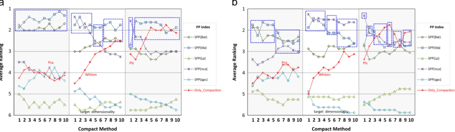
In order to have a more statistically meaningful picture of the previous results, we carried out a ranking analysis. This analysis consisted in ranking all the PP indexes together with the standalone compaction method (based on their associated 10-fold-CV average accuracies) for each particular combination of dataset, classification method, compaction method and target dimensionality. In cases of ties, we perform the correction suggested in[83], in which all methods in the tie are assigned a rank equivalent to the center of the positions they occupy in the ranking (for example, if two methods tied for second place, they are assigned to rank 2.5).Fig. 5shows the average corrected rankings for each classifier, compaction method and target dimension (averaged across datasets and experiment runs). The dashed boxes in the plots frame all those PP indexes that have no significant statistical difference with respect to the best placed index in the corresponding dimension. The statistical significance was assessed following the procedure described in [83], in which the non-parametric Friedman's test statistics is first employed to verify the existence of differences in performances of the indexes (we found that, for all dimensions, there exist significant differences at a significance level of 0.05). Next, we determined which methods are different from one another (in each target dimension) by using Dunn's technique (details in[83]). In this technique, multiple pairwise comparisons are performed corresponding to the different pairs of PP indexes. After Bonferroni correction of the significance levels of individual tests, we identified all PP indexes presenting no significance difference with respect to the best placed in the ranking (using an overall significance level4of 0.25) and framed them inFig. 5.
The results from the ranking analysis validated our findings in
Fig. 4. For the two classifiers used, a statistical significant advantage of
the proposed framework is observed (w.r.t. only compaction) using the non-supervised compaction methods and the indexes lda,Bat and occasionallynca(with whitening compaction), although the standa-lone whitening compaction tends to improve their relative positions with the increase of the target dimension. With the Pls compaction, we verify that the framework presents a significant advantage only at the first two and three target dimensions (with LDA and 3NN classifiers respectively). In the other dimensions, the standalone Pls method has no statistical difference from the best results of the framework (usually withldaindex in 3NN classifier andncaindex in LDA classifier). The qpc and Lp indexes always present the worst performances, very distant from the other indexes.
Fig. 6shows the results of the ranking analysis conducted on the proposed framework and some popular dimension reduction meth-ods. This time, each index-compaction framework configuration entered the analysis as an independent method, together with the eight dimension reduction methods indicated in Section4.1, totaliz-ing 23 methods in the analysis. The results show that, with both classifiers and in almost all target dimensions, some configuration of the proposed framework is the best positioned in the ranking. The exception is in 10 dimensions with the LDA classifier, where the standalone Pls method is thefirst, but not significantly different from the configurations PCA-Bat and PCA-lda. As a general trend, the configuration PCA-ldaprovides the best performance with the 3NN classifier among all tested method and target dimensions. Also, with that same classifier, the configurations PCA-Batand Pls-ldatend to be statistically indistinguishable from PCA-ldaconfiguration. With LDA classifier, the PCA-ldaconfiguration is also one of the best methods, tending to present accuracies not significantly different from the top ranked configuration (Whiten-nca). The standalone Pls method tends to present the best accuracies among the methods outside the framework, while the FS methods (ReliefF and Ttest) present poor results, which agrees with the claim[12]that FE is preferable over FS when the predictive accuracy is the most important factor.
Finally, to get a sense of the computational cost, we included in Fig. 6 the time used to run all experiments relative to each configuration/method. It is observed that the framework is more time consuming than the other methods. This is due to the optimization stage, which is a stochastic process. Nevertheless, the best performing configuration PCA-ldahas the lowest times among all configurations. In real situations, the framework would not be so delayed for a particular dataset (it is in the order of few seconds to get one dimension), since it is not necessary to perform all the experimenta-tion presented here. In addiexperimenta-tion, it is worth to menexperimenta-tion that the eight evaluated methods are well established and the toolboxes used for their implementations are computationally optimized.
Fig. 5.Average ranking results of the studied PP indexes for the two classifiers (averaged over datasets and experiment runs) as a function of the target dimensionality. The dotted boxes indicate all those PP indexes that have no significant statistical difference with respect to the best placed index in the corresponding dimension. (a) Ranking 3NN, (b) Ranking LDA.
4This number was suggested in[83], which is rather high because the risk of
obtained false significant differences is reduced due to the previous application of Friedman's test.
5. Conclusion
Reducing the dimensionality of datasets with large number of features and few examples is a challenging problem. In this paper we described and evaluated a Projection Pursuit framework, which is intended to circumvent the difficulties associated with that kind of data and to facilitate the construction of classifiers. The framework is formed by two stages: thefirst stage performs a rapid compaction of the data, which is used by the second stage to perform a projection search, seeking to optimize a measure of interestingness (the PP index). In an experimental study, comprising eight public microarray datasets and various framework configurations (varying the compac-tion method, PP index and target dimensionality), we showed that the proposed framework can effectivelyfind low dimensional repre-sentations of the data with good discriminatory properties. The framework, with Whitening or PCA compaction and PP indexeslda,
Bhattacharyaandnca, was able to outperform eight well established
dimension reduction methods in their ability to pack more discrimi-natory information into fewer dimensions.
We are planning to investigate more thoroughly the links between the properties of datasets and the performance of the different framework configurations, since we noted that the suitability of the configurations can vary across datasets. The aim would be the construction of a system that can select the best configuration of the framework for the problem at hand. Probably, a meta-learning approach[83]would be a good approach to this end. We also intend to apply the framework in other domains, like proteomics and astronomy datasets, where the imbalance between features and examples is even more aggravated.
Acknowledgments
We would like to thank CNPq (Conselho Nacional de Desen-volvimento Científico e Tecnológico) grant#151547/2013-0 and FAPESP (São Paulo Research Foundation) grant#2012/22295-0 for funding this study.
References
[1]I.M. Johnstone, D.M. Titterington, Statistical challenges of high-dimensional data INTRODUCTION, Philos. Trans. R. Soc. A—Math. Phys. Eng. Sci. 367 (1906) (2009) 4237–4253.
[2]S. Russell, L. Meadows, R. Russell, Microarray Technology in Practice, 1 ed., Elsevier/Academic Press, San Diego, USA, 2008.
[3]T.R. Golub, D.K. Slonim, P. Tamayo, C. Huard, M. Gaasenbeek, J.P. Mesirov, H. Coller, M.L. Loh, J.R. Downing, M.A. Caligiuri, C.D. Bloomfield, E.S. Lander, Molecular classification of cancer: class discovery and class prediction by gene expression monitoring, Science 286 (1999) 531–537.
[4]E. Segal, N. Friedman, N. Kaminski, A. Regev, D. Koller, From signatures to models: understanding cancer using microarrays, Nat. Genet. 37 (S) (2005) S38–S45.
[5]L. Jimenez, D. Landgrebe, Hyperspectral data analysis and supervised feature reduction via projection pursuit, IEEE Trans. Geosci. Remote Sens. 37 (6) (1999) 2653–2667.
[6]R. Clarke, H.W. Ressom, A. Wang, J. Xuan, M.C. Liu, E.A. Gehan, Y. Wang, The properties of high-dimensional data spaces: implications for exploring gene and protein expression data, Nat. Rev. Cancer 8 (1) (2008) 37–49.
[7]F. Korn, B. Pagel, C. Faloutsos, On the“dimensionality curse”and the“ self-similarity blessing”, IEEE Trans. Knowl. Data Eng. 13 (1) (2001) 96–111. [8]H. Liu, L. Yu, Toward integrating feature selection algorithms for classification
and clustering, IEEE Trans. Knowl. Data Eng. 17 (4) (2005) 491–502. [9]Y. Saeys, I.n. Inza, P. Larrañaga, A review of feature selection techniques in
bioinformatics, Bioinformatics 23 (19) (2007) 2507–2517.
[10]I. Guyon, S. Gunn, M. Nikravesh, L. Zadeh (Eds.), Feature Extraction, Founda-tions and ApplicaFounda-tions, Springer-Verlag New York, Inc., Secaucus, NJ, USA, 2006.
[11] C.J.C. Burges, Dimension reduction: a guided tour, Found. Trends Mach. Learn., Now Publishers Inc., Hanover, MA, USA, 2 (4).
[12]H. Liu, H. Motoda, Feature Extraction, Construction and Selection: A Data Mining Perspective, Kluwer Academic Publishers, Now Publishers Inc., Han-over, MA, USA, 1998.
[13]J.H. Friedman, J.W. Tukey, A projection pursuit algorithm for exploratory data analysis, IEEE Trans. Comput. 23 (9) (1974) 881–890.
[14]J.H. Friedman, Exploratory projection pursuit, Am. Stat. Assoc. 82 (397) (1987) 249–266.
[15]W. Huang, X. Zhang, Projection pursuitflood disaster classification assessment method based on multi-swarm cooperative particle swarm optimization, J. Water Resour. Prot. 3 (6) (2011) 415–420.
[16]S. Wang, X. Zhang, Projection pursuit dynamic cluster model and its applica-tion to water resources carrying capacity evaluaapplica-tion, J. Water Resour. Prot. 2 (5) (2010) 2474–2482.
[17]J.A. Malpica, J.G. Rejas, M.C. Alonso, A projection pursuit algorithm for anomaly detection in hyperspectral imagery, Pattern Recognit. 41 (2008) 3313–3327. [18]X. Cui, R. Jin, Xu. Asghar, P. Condamine, J.T. Svensson, S. Wanamaker,
N. Stein, I. Roose, T.J. Close, Detecting single-feature polymorphisms using oligonucleotide arrays and robustified projection pursuit, Bioinformatics 21 (20) (2005) 3852–3858.
Fig. 6.Average ranking results (averaged over datasets and replicate runs) and computational times of 15 configurations of the framework (three compaction methods and
five PP indexes) and eight well-known dimension reduction methods, evaluated with classifiers 3NN and LDA. Boldface numbers indicate the best results in the respective target dimension. Shaded boxes indicate the positions in the ranking that are not significantly different from the best position in the corresponding dimension.
[19]D. Pena, F. Prieto, Cluster identification using projections, J. Am. Stat. Assoc. 96 (456) (2001) 1433–1445.
[20]R. Bolton, W. Krzanowski, Projection pursuit clustering for exploratory data analysis, J. Comput. Graph. Stat. 12 (1) (2003) 121–142.
[21]E. Lee, D. Cook, S. Klinke, T. Lumley, Projection pursuit for exploratory supervised classification, J. Comput. Graph. Stat. 14 (4) (2005) 831–846. [22]O. Demirci, V.P. Clark, V.D. Calhoun, A projection pursuit algorithm to classify
individuals using fMRI data: application to schizophrenia, Neuroimage 39 (4) (2008) 1774–1782.
[23]A.M. Pires, J.A. Branco, Projection-pursuit approach to robust linear discrimi-nant analysis, J. Multivar. Anal. 101 (10) (2010) 2464–2485.
[24]M. Grochowski, W. Duch, Fast projection pursuit based on quality of projected clusters, in: A. Dobnikar, U. Lotric, B. Ster (Eds.), Adaptive and Natural Computing Algorithms Lecture Notes in Computer Science, vol. 6594, Springer, Berlin, Heidelberg, 2011, pp. 89–97.
[25]Y. Ren, H. Liu, X. Yao, M. Liu, Prediction of ozone tropospheric degradation rate constants by projection pursuit regression, Anal. Chim. Acta 589 (1) (2007) 150–158.
[26]M. Aladjem, Projection pursuit mixture density estimation, IEEE Trans. Signal Process. 53 (11) (2005) 4376–4383.
[27]J.R. Jee, Projection pursuit, Wiley Interdiscip. Rev.: Comput. Stat. 1 (2) (2009) 208–215.
[28]E. Rodriguez-Martinez, J.Y. Goulermas, T. Mu, J.F. Ralph, Automatic induction of projection pursuit indices, IEEE Trans. Neural Netw. 21 (8) (2010) 1281–1295. [29]P.J. Huber, Projection pursuit, Ann. Stat. 13 (2) (1985) 435–475.
[30]M.C. Jones, R. Sibson, What is projection pursuit? J. R. Stat. Soc. Ser. A: General 150 (1) (1987) 1–37.
[31]G. Nason, Three-dimensional projection pursuit, J. R. Stat. Soc. Ser. C 44 (1995) 411–430.
[32]Q. Guo, W. Wu, F. Questier, D. Massart, C. Boucon, S. de Jong, Sequential projection pursuit using genetic algorithms for data mining of analytical data, Anal. Chem. 72 (13) (2000) 2846–2855.
[33]S. Espezua, E. Villanueva, C.D. Maciel, Towards an efficient genetic algorithm optimizer for sequential projection pursuit, Neurocomputing 123 (2014) 40–48.
[34]B. Webb-Robertson, K. Jarman, S. Harvey, C. Posse, B. Wright, An improved optimization algorithm and Bayes factor termination criterion for sequential projection pursuit, Chemom. Intell. Lab. Syst. 77 (1–2) (2005) 149–160. [35]A. Berro, S.L. Marie-Sainte, A. Ruiz-Gazen, Genetic algorithms and particle
swarm optimization for exploratory projection pursuit, Ann. Math. Artif. Intell. 60 (1–2, SI) (2010) 153–178.
[36]J. Kruskal, Toward a practical method which helps uncover the structure of a set of multivariate observations byfinding the linear transformation which optimizes a new“Index of Condensation”, Stat. Comput. (1969) 427–440. [37] G. Nason, Design and choice of projection indices (Ph.D. thesis), University of
Bath, 1992.
[38]C. Posse, Projection pursuit exploratory data analysis, Comput. Stat. Data Anal. 20 (1995) 669–687.
[39]C. Posse, Tools for two-dimensional exploratory projection pursuit, J. Comput. Graph. Stat. 4 (2) (1995) 83–100.
[40] S.L. Marie-Sainte, A. Berro, A. Ruiz-Gazen, An efficient optimization method for revealing local optima of projection pursuit indices, in: ANTS Conference, 2010, pp. 60–71.
[41]K. Zhang, L.-W. Chan, Dimension reduction as a deflation method in ICA, IEEE Sign. Process. Lett. 13 (1) (2006) 45–48.
[42]I. Perisic, C. Posse, Projection pursuit indices based on the empirical distribu-tion funcdistribu-tion, J. Comput. Graph. Stat. 14 (3) (2005) 700–715.
[43]D. Cook, A. Buja, J. Cabrera, Projection pursuit indexes based on orthonormal function expansions, J. Comput. Graph. Stat. 2 (3) (1993) 225–250. [44] M. Grochowski, W. Duch, Projection pursuit constructive neural networks
based on quality of projected clusters, in: V. Kurkova, R. Neruda, J. Koutnik (Eds.), Artificial Neural Networks—ICANN 2008, PT II, Lecture Notes In Computer Science, vol. 5164, 2008, pp. 754–762.
[45]E.-K. Lee, D. Cook, A projection pursuit index for large p small n data, Stat. Comput. 20 (3) (2010) 381–392.
[46]J.H. Friedman, W. Stuetzle, Projection pursuit regression, J. Am. Stat. Assoc. 76 (1981) 817–823.
[47]P. Hall, On projection pursuit regression, Ann. Stat. 17 (2) (1989) 573–588. [48] J. Goldberger, S. Roweis, G. Hinton, R. Salakhutdinov, Neighbourhood
compo-nents analysis, in: Advances in Neural Information Processing Systems, vol. 17, 2005, pp. 513–520.
[49]W. Yang, K. Wang, W. Zuo, Fast neighborhood component analysis, Neuro-computing 83 (2012) 31–37.
[50] H.V. Nguyen, L. Bai, Face verification using indirect neighbourhood compo-nents analysis, in: Proceedings of the 6th International Conference on Advances in Visual Computing—Volume Part II, ISVC'10, Springer-Verlag, Berlin, Heidelberg, 2010, pp. 637–646.
[51] A. Khandelwal, P. Choudhury, R. Sarkar, S. Basu, M. Nasipuri, N. Das, Text line segmentation for unconstrained handwritten document images using neigh-borhood connected component analysis, in: Proceedings of the 3rd Interna-tional Conference on Pattern Recognition and Machine Intelligence, PReMI '09, Springer-Verlag, Berlin, Heidelberg, 2009, pp. 369–374.
[52]X. He, S. Yan, Y. Hu, P. Niyogi, H. Jiang Zhang, Face recognition using Laplacianfaces, IEEE Trans. Pattern Anal. Mach. Intell. 27 (2005) 328–340.
[53] M. Asuncion Vicente, P.O. Hoyer, A. Hyvarinen, Equivalence of some common linear feature extraction techniques for appearance-based object recognition tasks, IEEE Trans. Pattern Anal. Mach. Intell. 29 (5) (2007) 896–900. [54] W. Deng, Y. Liu, J. Hu, J. Guo, The small sample size problem of ICA: a
comparative study and analysis, Pattern Recognit. 45 (12) (2012) 4438–4450. [55] S. Biswas, J. Storey, J. Akey, Mapping gene expression quantitative trait loci by singular value decomposition and independent component analysis, BMC Bioinform. 9 (1) (2008) 244.
[56] P. Cunningham, Dimension Reduction, Technical Report, 2007.
[57]D. DiPietroPaolo, H.-P. Mller, G. Nolte, S.N. Ern, Noise reduction in magneto-cardiography by singular value decomposition and independent component analysis, Med. Biol. Eng. Comput. 44 (6) (2006) 489–499.
[58] R. Shen, D. Ghosh, A. Chinnaiyan, Z. Meng, Eigengene-based linear discrimi-nant model for tumor classification using gene expression microarray data, Bioinformatics 22 (21) (2006) 2635–2642.
[59] O. Alter, P.O. Brown, D. Botstein, Generalized singular value decomposition for comparative analysis of genome-scale expression data sets of two different organisms, Proc. Natl. Acad. Sci. 100 (6) (2003) 3351–3356.
[60] M. Wall, A. Rechtsteiner, L. Rocha, Singular value decomposition and principal component analysis, in: A Practical Approach to Microarray Data Analysis, 2003, pp. 91–109.
[61]O. Alter, P.O. Brown, D. Botstein, Singular value decomposition for genome-wide expression data processing and modeling, Proc. Natl. Acad. Sci. 97 (18) (2000) 10101–10106.
[62] I. Jolliffe, Principal Component Analysis, Springer, New York, NY, 1986. [63]T.S. Nguyen, J. Rojo, Dimension reduction of microarray gene expression data: the
accelerated failure time model, J. Bioinform. Comput. Biol. 7 (6) (2009) 939–954. [64] R. Rosipal, N. Krmer, Overview and recent advances in partial least squares, in: Lecture Notes in Computer Science (including subseries Lecture Notes in Artificial Intelligence and Lecture Notes in Bioinformatics), vol. 3940, 2006, pp. 34–51, cited by (since 1996)132.
[65] Y. Su, S. Shan, X. Chen, W. Gao, Classifiability-based discriminatory projection pursuit, IEEE Trans. Neural Netw. 22 (12) (2011) 2050–2061.
[66] S.L. Pomeroy, P. Tamayo, M. Gaasenbeek, L.M. Sturla, M. Angelo, M.E. Mclaughlin, J.Y.H. Kim, L.C. Goumnerova, P.M. Black, C. Lau, J.C. Allen, D. Zagzag, J.M. Olson, T. Curran, C. Wetmore, J.A. Biegel, T. Poggio, S. Mukherjee, R. Rifkin, A. Califano, G. Stolovitzky, D.N. Louis, J.P. Mesirov, E.S. Lander, T.R. Golub, Prediction of central nervous system embryonal tumour outcome based on gene expression, Nature 415 (6870) (2002) 436–442.
[67] C.L. Nutt, D.R. Mani, R.A. Betensky, P. Tamayo, J.G. Cairncross, C. Ladd, U. Pohl, C. Hartmann, M. Mclaughlin, Gene expression-based classification of malig-nant gliomas correlates better with survival than histological classification, Cancer Res. 63 (2003) 1602–1607.
[68] U. Alon, N. Barkai, D.A. Notterman, K. Gishdagger, S. Ybarradagger, D. Mackdagger, A.J. Levine, Broad patterns of gene expression revealed by clustering analysis of tumor and normal colon tissues probed by oligonucleo-tide arrays, Proc. Natl. Acad. Sci. USA 96 (12) (1999) 6745–6750.
[69] M.A. Shipp, K.N. Ross, P. Tamayo, A.P. Weng, J.L. Kutok, R.C. Aguiar, M. Gaasenbeek, M. Angelo, M. Reich, G.S. Pinkus, T.S. Ray, M.A. Koval, K.W. Last, A. Norton, T.A. Lister, J. Mesirov, D.S. Neuberg, E.S. Lander, J.C. Aster, T.R. Golub, Diffuse large B-cell lymphoma outcome prediction by gene-expression profiling and supervised machine learning, Nat. Med. 8 (1) (2002) 68–74.
[70] S.A. Armstrong, J.E. Staunton, L.B. Silverman, R. Pieters, M.L. den Boer, M.D. Minden, S.E. Sallan, E.S. Lander, T.R. Golub, S.J. Korsmeyer, MLL transloca-tions specify a distinct gene expression profile that distinguishes a unique leukemia, Nat. Genet. 30 (2002) 41–47.
[71]D. Singh, P.G. Febbo, K. Ross, D.G. Jackson, J. Manola, C. Ladd, P. Tamayo, A.A. Renshaw, A.V. D'Amico, J.P. Richie, E.S. Lander, M. Loda, P.W. Kantoff, T.R. Golub, W.R. Sellers, Gene expression correlates of clinical prostate cancer behavior, Cancer Cell 1 (2) (2002) 203–209.
[72] J. Khan, J.S. Wei, M. Ringner, L.H. Saal, M. Ladanyi, F. Westermann, F. Berthold, M. Schwab, C.R. Antonescu, C. Peterson, P.S. Meltzer, Classification and diagnostic prediction of cancers using gene expression profiling and artificial neural networks, Nat. Med. 7 (6) (2001) 673–679.
[73]M.P.R. Berry, C.M. Graham, F.W. McNab, Z. Xu, S.A.A. Bloch, T. Oni, K.A. Wilkinson, R. Banchereau, J. Skinner, R.J. Wilkinson, C. Quinn, D. Blankenship, R. Dhawan, J.J. Cush, A. Mejias, O. Ramilo, O.M. Kon, V. Pascual, J. Banchereau, D. Chaussabel, A. O/'Garra, An interferon-inducible neutrophil-driven blood transcriptional signature in human tuberculosis, Nature 466 (7309) (2010) 973–977.
[74]S. Dudoit, J. Fridlyand, T.P. Speed, Comparison of discrimination methods for the classification of tumors using gene expression data, J. Am. Stat. Assoc. 97 (457) (2002) 77–87.
[75] C.M. Bishop, Pattern Recognition and Machine Learning (Information Science and Statistics), Springer-Verlag, New York, Inc, 2006.
[76] MATLAB, version 7.10.0 (R2010a), The MathWorks Inc., 2010.
[77] S.T. Roweis, L.K. Saul, Nonlinear dimensionality reduction by locally linear embedding, Science 290 (2000) 2323–2326.
[78] H.-M. Wu, Kernel sliced inverse regression with applications to classification, J. Comput. Graph. Stat. 17 (3) (2008) 590–610.
[79] N. Zhou, L. Wang, A modified T-test feature selection method and its application on the hapmap genotype data, Genomics Proteomics Bioinform. 5 (3–4) (2007) 242–249.
[80]I. Kononenko, Estimating attributes: analysis and extensions of RELIEF, in: F. Bergadano, L.D. Raedt (Eds.), European Conference on Machine Learning, Springer-Verlag New York, Inc., Secaucus, NJ, USA, 1994, pp. 171–182. [81] L. van der Maaten, E.O. Postma, H.J. van den Herik, Dimensionality Reduction:
A Comparative Review, Technical Report, Tilburg University, 2009.
[82] I.H. Witten, E. Frank, L. Trigg, M. Hall, G. Holmes, S.J. Cunningham, Weka: Practical Machine Learning Tools and Techniques with Java Implementations,
http://www.cs.waikato.ac.nz/ml/weka/, 1999.
[83]P.B. Brazdil, C. Soares, J.P. Da Costa, Ranking learning algorithms: using IBL and meta-learning on accuracy and time results, Mach. Learn. 50 (3) (2003) 251–277.
Soledad Espezuais currently a Postdoctoral fellow in the Department of Computer Science at the University of São Paulo, Brazil. Her major research focuses are Evolutionary Computation, Bioinformatics, Machine Learning, Data Mining and Meta-learning. She received his Ph.D. and M.Sc. degrees in electrical engineering from the University of São Paulo, Brazil, in 2008 and 2013 respectively.
Edwin Villanuevareceived his M.Sc. and Ph.D. degrees in electrical engineering from the University of São Paulo, Brazil, in 2007 and 2012 respectively. He is currently a Postdoctoral fellow in the Department of Computer Science at the University of São Paulo, Brazil. His main interests are Machine Learning, Data Mining, Meta-learning, Bioinformatics, Evolutionary Computa-tion, Bioinspired Computing, Optimization and Prob-abilistic Graphical Models.
Carlos D. Macielis an Associate Professor in Statistical Signal Processing and Pattern Recognition at the Department of Electrical Engineering, University of São Paulo (USP) at Sao Carlos, Brazil. He received his B.Sc. from the Military Institute of Engineering (IME), Brazil, in 1989 and Ph.D. degree from the Federal University of Rio de Janeiro (UFRJ), Brazil, in 2000.
André Carvalhois a Full Professor in the Department of Computer Science at the University of São Paulo, Brazil. He received his Ph.D. in Electronics from the University of Kent, UK, in 1994. He co-authored one textbook on neural networks and one on artificial intelligence, both in Portuguese. He has several publications in books, refereed journals and conferences. He is in the editorial board and was a guest editor for international journals and general program chair of several national and international conferences. He gave invited talks and won the best paper awards in national and interna-tional conferences. He collaborates with researchers from Brazil and abroad in several research projects.