Direct simulation of electron transfer using ring polymer molecular
dynamics: Comparison with semiclassical instanton theory and exact
quantum methods
Artur R. Menzeleev, Nandini Ananth, and Thomas F. Miller IIIa)
Division of Chemistry and Chemical Engineering, California Institute of Technology, Pasadena, California 91125, USA
(Received 11 July 2011; accepted 25 July 2011; published online 17 August 2011)
The use of ring polymer molecular dynamics (RPMD) for the direct simulation of electron transfer (ET) reaction dynamics is analyzed in the context of Marcus theory, semiclassical instanton theory, and exact quantum dynamics approaches. For both fully atomistic and system-bath representations of condensed-phase ET, we demonstrate that RPMD accurately predicts both ET reaction rates and mechanisms throughout the normal and activationless regimes of the thermodynamic driving force. Analysis of the ensemble of reactive RPMD trajectories reveals the solvent reorganization mecha-nism for ET that is anticipated in the Marcus rate theory, and the accuracy of the RPMD rate calcula-tion is understood in terms of its exact descripcalcula-tion of statistical fluctuacalcula-tions and its formal conneccalcula-tion to semiclassical instanton theory for deep-tunneling processes. In the inverted regime of the ther-modynamic driving force, neither RPMD nor a related formulation of semiclassical instanton theory capture the characteristic turnover in the reaction rate; comparison with exact quantum dynamics sim-ulations reveals that these methods provide inadequate quantization of the real-time electronic-state dynamics in the inverted regime.© 2011 American Institute of Physics. [doi:10.1063/1.3624766]
I. INTRODUCTION
Condensed-phase electron transfer (ET) reactions are central to many biological and synthetic pathways for energy conversion and catalysis.1–4The development of accurate, ro-bust, and scalable methods for the study of such reactions is thus a key objective in theoretical chemistry. Although transi-tion state theories and rate models for ET have been success-fully applied in complex systems,5–8 methods for the direct simulation and mechanistic study of ET dynamics in general systems remain less fully developed. To this end, we explore the use of ring polymer molecular dynamics (RPMD) for the description of prototypical ET reactions between mixed-valence transition metal ions in water, and we compare the RPMD approach against benchmark semiclassical and quan-tum dynamics methods.
Fundamental theoretical challenges in the direct sim-ulation of ET reactions arise due to the coupling of the intrinsically quantum mechanical electronic transitions with slower, classical motions of the surrounding environment. Numerous semiclassical and mixed quantum-classical dy-namics methods have been developed for the investigation of electronically non-adiabatic reactions,9–19 but existing methods do not enable mechanistic studies that are inde-pendent of dividing surface assumptions in general systems; nor do they yield dynamical trajectories that preserve the equilibrium Boltzmann distribution20,21and allow for the use of rare-event sampling methodologies.22 New methods are
a)Electronic mail: [email protected].
needed to accurately describe coupled electronic and nuclear dynamics and to enable the efficient and robust simulation of long trajectories that bridge the multiple timescales of ET reactions in complex systems.
RPMD (Ref. 23) is an approximate quantum dynamical method that is based on the imaginary-time path integral for-mulation of statistical mechanics.24,25 It provides an isomor-phic classical molecular dynamics model for the real-time evolution of a quantum mechanical system. Previous appli-cations of RPMD include studies of molecular liquids,26–31 hydrogen transfer rates,32–35 and tunneling processes in low-dimensional systems.36–38A key feature of the RPMD method is that it yields real-time molecular dynamics trajectories that preserve the exact quantum Boltzmann distribution and exhibit time-reversal symmetry.23,39 These properties allow RPMD to be used in combination with rare-event sampling methods for the trajectory-based analysis of quantum me-chanical tunneling processes in systems involving thousands of atoms.35,40 We have recently extended RPMD to describe electronic and nuclear dynamics, including solvated electron diffusion41 and non-adiabatic electron injection into liquid water.40
In the current paper, RPMD is used to directly simu-late ET dynamics in both atomistic and system-bath represen-tations for mixed-valence ET in water. The calculated rates and mechanisms are analyzed in the context of semiclassical and exact quantum methods. A description of the employed methodologies is provided in Sec.II, and Sec.IIIpresents the details of the atomistic and system-bath representations. Cal-culation details are given in Sec.IV, and a discussion of the results is presented in Sec.V.
II. METHODS
Several methods are utilized to investigate ET rates and mechanisms, including RPMD, semiclassical instanton the-ory (SCI), exact quantum-mechanical dynamics, and the clas-sical Marcus rate theory for ET. These methods are summa-rized below.
A. Ring polymer molecular dynamics
The RPMD equations of motion for a quantized electron andNclassical particles are23,41
˙ v(α) =ω2n(q(α+1)+q(α−1)−2q(α)) − 1 me ∇q(α)Uext(q(α),Q1, . . . ,QN) (1) and ˙ Vj = − 1 nMj n α=1 ∇QjUext(q (α),Q1, . . . ,Q N), (2)
where q(α) andv(α) are the position and velocity vectors of αth ring polymer bead,Qj andVj are the position and veloc-ity vectors of the jth classical particle, andnis the number of imaginary-time ring-polymer beads. The intra-bead har-monic frequency isωn/(β¯), whereβ is the reciprocal tem-perature. The masses of electron and classical particles are meandMj, respectively,Uext(q(α),Q1, . . . ,QN) is the
poten-tial energy function of the system, andq(0)=q(n). Equations (1)and(2) generate a classical dynamics that we employ as a model for the real-time dynamics of the system.41 In the limit of largen, these dynamics preserve the exact Boltzmann distribution.39
As in classical formulations of the thermal rate constant,42–44the RPMD rate can be expressed as32,38
kRPMD= lim
t→∞κ(t)kTST. (3) Here, kTST is the transition state theory (TST)
approxima-tion for the rate for a dividing surface ξ(r)=ξ‡, where ξ(r) is a collective variable,r= {q(1), . . . ,q(n),Q}is the full
position vector for the system, and Q= {Q1, . . . ,QN} de-notes the set of classical particle positions. The prefactor, κ(t), is the time-dependent transmission coefficient that ac-counts for the recrossing of trajectories through the divid-ing surface. An important feature of RPMD is that calcu-lated rates and mechanisms are independent of the choice of TST dividing surface, as in exact quantum and exact classical dynamics.32,38,45
The TST rate in Eq.(3)is calculated using33,46,47 kTST=(2πβ)−1/2gξc
e−βF(ξ‡)
ξ‡
−∞dξ e−βF(ξ)
. (4)
Here,F(ξ) is the free energy (FE) alongξ:
e−βF(ξ)= δ(ξ(r)−ξ
)
δ(ξ(r)−ξr)
, (5)
whereξris a reference point in the reactant region, and48–50
gξ(r)= d i=1 1 mi ∂ξ(r) ∂ri 21/2 . (6)
The scalarri ∈ {r}in this equation indicates either a ring-polymer or classical particle degree of freedom, mi is the corresponding mass, andd is the total number of degrees of freedom in the system. In Eqs.(4)and(5),. . . denotes the equilibrium ensemble average,
. . . =
drdve−βHn(r,v)(. . .)
drdve−βHn(r,v) , (7)
and. . .cdenotes the average in the constrained ensemble
. . .c= drdve−βHn(r,v)(. . .)δ(ξ(r)−ξ‡) dr dve−βHn(r,v)δ(ξ(r)−ξ‡) . (8) Here, Hn(r,v)= N j=1 1 2MjV 2 j + n α=1 1 2mb(v (α))2+Un(r), (9)
where mb is the fictitious Parrinello-Rahman mass,39 v= {v(1), . . . ,v(n),V1, . . . ,VN}, and Un(r)= 1 n n α=1 1 2meω 2 n(q( α)−q(α−1))2 +1 n n α=1 Uext(q(α),Q) (10)
is the full potential energy function for the ring polymer. The transmission coefficient in Eq.(3) is obtained from the flux-side correlation function using
κ(t)= ξ˙0h(ξ(rt)−ξ
‡) c
ξ˙0h( ˙ξ0)c
, (11)
whereh(ξ) is the Heaviside function, ˙ξ0is the initial velocity of the collective variable in an RPMD trajectory released from the dividing surface, andrtis the time-evolved position of the system along that trajectory.33
B. Semiclassical instanton theory
The “Im F” premise in semiclassical rate theory relates the thermal rate constant in the deep-tunneling regime to the analytical continuation of the partition function into the com-plex plane,51–56
k≈ 2
β¯QrImR, (12) where Qr is the reactant partition function and ImR is the imaginary part of the analytical continuation of the partition function for the full system. In the steepest-descent limit, the “Im F” description is equivalent to the flux-side time correla-tion formulacorrela-tion of SCI theory.57,58We adapt this approach to describe the transfer of a single quantized electron in a classi-cal solvent.
The partition function for the full system in the ring-polymer representation can be expressed as
Qn=c dQIn(Q), (13) wherec= Nj=1 Mj 2πβ¯2, In(Q)= meωn 2π¯ −n/2 d{q(α)}e−A({q(α)};Q)/¯, (14) and A({q(α)};Q)=(β¯)Un(r) (15) is the classical action for a periodic trajectory in imaginary time. The notation presented here assumes that the quantized electron moves in a single dimension. At each solvent config-uration, the steepest-descent approximation to In(Q) is ob-tained by expanding A({q(α)};Q) to second order about its
global minimum {q˜(α)}, for which the electron ring-polymer
coordinates obey the following stationary condition: 1 n n α=1 ∂q∂(α)Uext(q (α),Q)| q(α)=q˜(α) −ω2n( ˜q(α+1)+q˜(α−1)−2 ˜q(α))=0. (16) The steepest-descent approximation yields
In(Q)= √ 1 detKe
−A({q˜(α)};Q)/¯
, (17)
whereKis the Hessian matrix given by Kμν= ωn ¯ ∂2 ∂q(μ)∂q(ν)A({q˜ (α)};Q)| {q(α)}={q˜(α)}, (18)
and where (det K)= ni=1η2i is obtained from the normal mode frequencies,{ηi}.
For a reaction with a barrier, a saddle point satisfies the stationary condition in Eq. (16), and the Hessian matrix ex-hibits an imaginary normal-mode frequency,η1. By analyti-cally continuingη1onto the real axis, and by integrating out the zero-frequency normal mode that is associated with the cyclic permutation of the ring-polymer beads, we obtain the steepest-descent SCI rate:58
kSCI = c Qr dQIn(Q), (19) where In(Q)= meBnωn3 2π¯ 1/2 1 √ detKe −A({q˜(α)};Q)/¯ , (20)
(detK)= |ηi|2is obtained from a product that excludes the zero-frequency mode, and
Bn= n
α=1
( ˜q(α+1)−q˜(α))2. (21) Formal connections between path-integral statistics and reactive tunneling have long been recognized.25,58–62 In par-ticular, Althorpe and co-workers37 have recently emphasized the connection between the TST limit of RPMD and the re-versible action work (RAW) formulation of SCI theory.51,63
To the extent that Eq. (19)is an harmonic approximation to the RAW SCI formulation,37
kRPMD= κ o α kSCI, (22)
where α=2π(β¯|η1|)−1, andκo is the transmission
coeffi-cient through a dividing surface that minimizes the recrossing of RPMD trajectories.
C. Exact quantum dynamics
We obtain numerically exact quantum dynamics for ET using the quasi-adiabatic path integral (QUAPI) method.64–68 The method is applied to a redox system composed of two diabatic electronic states and a coordinate representing polar-ization of the solvent dipole field; the solvent coordinate is in turn linearly coupled to a harmonic oscillator bath.
The Hamiltonian for the redox system is65 HS= p2 s 2ms + V11(s) V12(s) V12(s) V22(s) , (23)
wheresis the solvent coordinate,psis the conjugate momen-tum, and ms is the effective solvent mass. Here,V11(s) and
V22(s) are diabatic states corresponding to reactant and
prod-uct states for ET, and V12(s) is the electronic coupling. The
Hamiltonian describing the bath modes and their coupling to the solvent coordinate is
HB= f j=1 P2 j 2Mj + f j=1 1 2Mjω 2 j Qj− cjs Mjω2j 2 , (24)
whereMj,ωj, andQj are the mass, frequency, and the posi-tion of thejth bath mode, respectively, andcj is the strength of the coupling between the jth bath mode and the solvent coordinate.
The exact quantum mechanical rate constant can be ex-pressed in terms of the symmetrized real-time flux-flux (FF) correlation function,69 kQ= lim t→∞ 1 Qr t 0 CFF(t)dt, (25) where CFF(t)=Tr[FeiH t ∗ c/¯Fe−iH tc/¯], (26)
andQris the reactant partition function. Here,H =HS+HB
is the full ET Hamiltonian, F =i/¯[H,P2] is the
opera-tor for the flux between the reactant and product electronic states,P2= |22|is the projection operator for the product
electronic state, andtc=t−iβ¯/2 is the complex time. The
propagators are discretized intoN time slices of lengthtc,
and the trace in Eq.(26)is expanded to yield CFF(t)= ∞ −∞dQ0Q0| s1, σ1|F|s2N+2, σ2N+2 × 2N+2 k=N+3 σk, sk|eiH t ∗ c/¯|σk −1, sk−1 × sN+2, σN+2|F|sN+1, σN+1
×N+
1
k=2
σk, sk|e−iH tc/¯|σk−1, sk−1 |Q0, (27)
where Q0 represents the bath degrees of freedom,sk is the solvent coordinate, and σkis the electronic state at complex time slicek.
The propagators in Eq. (27) are factorized using the quasi-adiabatic short-time approximation:64
e−iH tc/¯≈e−iHBtc/2¯e−iHStc/¯e−iHBtc/2¯. (28)
Analytical integration over the bath modes then yields CFF(t)= 1 ¯2Re [C1(2,2,1,1;tc)−C2(2,1,2,1;tc) +C3(1,1,2,2;tc)−C4(1,2,1,2;tc)], (29) where Ci(σ1, σN+1, σN+2, σ2N+2;tc) = ds1· · · dsN dsN+2· · · ds2N+1 × 2 σ2=1 · · · 2 σN=1 2 σN+3=1 · · · 2 σ2N+1=1 Ii(s,σ;tc) (30) and Ii(s,σ;tc)=V12(s1)V12(sN+2)K(s,σ;tc)I(s). (31)
Here,s2N+2=s1,sN+2=sN+1, and we have introduced the
notations= {s1, . . . , s2N+2}andσ = {σ1, . . . , σ2N+2}.
In Eq.(31), the path-integral expression for the complex-time propagators of the system Hamiltonian is given by
K(s,σ;tc)= 2N+2 k=N+3 σk, sk|eiHSt ∗ c/¯|σ k−1, sk−1 ×N+ 1 k=2 σk, sk|e−iHStc/¯|σk−1, sk−1. (32)
The matrix elements in Eq. (32)are obtained using the nu-merically exact expression
sk, σk|e−iHStc/¯|sk−1, σk−1 = M0 m=1 φm(sk, σk)φm∗(sk−1, σk−1)e−iEmtc/¯, (33)
whereφm(s, σ) andEmare the eigenstates and eigenenergies of HS, respectively, andM0 is the number of eigenstates in-cluded in the expansion.
The discretized form of the non-local influence func-tional in Eq.(31), which accounts for bath-induced electronic transitions in the system, is
I(s)=I0exp − 2N+2 k=1 k k=1 Bkksk sk , (34)
where I0 is the partition function of the uncoupled bath
oscillators.64,70,71 The diagonal elements of {B
kk} describe local contributions to the bath response function from a par-ticular complex time slicekalong the adiabatic path, and the
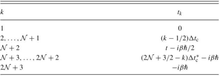
TABLE I. Complex timestkused to calculate the{Bkk}.
k tk 1 0 2, . . . ,N+1 (k−1/2)tc N+2 t−iβ¯/2 N+3, . . . ,2N+2 (2N+3/2−k)tc∗−iβ¯ 2N+3 −iβ¯
off-diagonal elements describe non-local contributions. For the case of linear system-bath coupling, the diagonal matrix elements are given by
Bkk = f j=1 c2j Mjω3jsinh(βωj/2) sin ωj(tk+1−tk) 2 ×sin ωj(tk+1−tk+iβ) 2 , (35)
and the off-diagonal matrix elements are given by Bkk = f j=1 c2 j Mjωj3sinh(βωj/2) sin ωj(tk+1−tk) 2 ×cos ωj(tk+1−tk+1+tk−tk+iβ) 2 ×sin ωj(tk+1−tk) 2 . (36)
The complex times tk in Eqs.(35)and(36)are provided in TableI.
D. Marcus theory for ET in a classical solvent
In the Marcus theory for ET,3,72–74electronic transitions occur at solvent geometries for which the donor and acceptor electronic states are isoenergetic. In the limit of weak elec-tronic coupling and classical solvent motions, the ET rate is thus kMT= 2π ¯ |V12| 2 β 4π λ 1/2 e−βG∗, (37)
whereV12is the electronic coupling matrix element,
G∗= (G
0+λ)2
4λ , (38)
λis the solvent reorganization energy, and−G0is the
ther-modynamic driving force for the ET reaction. The rate ex-pression in Eq. (37) exhibits three distinct regimes as the driving force is varied relative to λ. In the normal regime, where −G0< λ, the rate increases with increasing driv-ing force. A turnover in this trend occurs in the activation-less regime, for which−G0≈λ. In the inverted regime, for which−G0> λ, the rate decreases with increasing driving
force.
In the current study, we use implementations for Marcus theory, SCI theory, and RPMD in which the solvent degrees of freedom are treated classically; the role of nuclear quantum
TABLE II. Parameters for the atomistic representation of ET. Parameter Value QA/Å (0,0,−3.25) QD/Å (0,0,3.25) rH cut/Å 1.0 rM cut/Å 1.1 qO/e −0.84 qH/e 0.42 qM/e 3.0 γO/ (kcal/mol Å9) 6392.7
effects in diminishing the degree of turnover for the ET rate in the inverted regime3,75is not considered here.
III. SYSTEMS
ET dynamics is studied using both all-atom and system-bath representations for mixed-valence transition metal ions in water. These representations are described in the current section.
A. Atomistic representation for ET
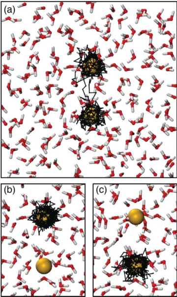
The atomistic representation for the ET reaction (Fig.1) is described using the potential energy function76
Uext(q,Q)=Usol(Q)+Ue-sol(q,Q)
+Ue-M(q,Q)+UM-sol(Q), (39)
whereqis the electron position andQis the set ofNclassical solvent atom positions. Solvent-solvent interactions,Usol(Q),
are described using the simple point charge (SPC) model77for explicit, rigid water molecules. The remaining interactions are described below, with the values of the parameters provided in TableII.
The electron-water interactions are described using the pairwise pseudopotential78 Ue-sol(r)= N k=1 Ue-solk (rk),
where rk= |q−Qk|. For cases in which the atom index k corresponds to a hydrogen atom,
Ue-solk (rk)= ⎧ ⎪ ⎪ ⎨ ⎪ ⎪ ⎩ − qHe 4π ε0rcutH , rk ≤rcutH − qHe 4π ε0rk , rk > rcutH , (40)
and whenkcorresponds to an oxygen atom, Ue-solk (rk)= − qOe
4π ε0rk
. (41)
Electron-ion interactions are described using
Ue-M(q)=Ue-D(|q−QD|)+Ue-A(|q−QA|), (42)
whereQDandQAdenote the respective positions of the donor
and acceptor metal ions, which are held fixed at a separation of 6.5 Å. These interactions are described using Shaw-type
FIG. 1. Snapshots of the atomistic representation for the ET reaction, with the donor and acceptor metal ions shown in yellow, the electron ring polymer in black, and the water molecules in red and white. Typical configurations of the symmetric ET system are presented with the electron ring polymer (a) in transition between the redox sites, (b) in the reactant basin, and (c) in the product basin.
pairwise pseudopotentials.79For the acceptor metal ion,
Ue-A(r)= ⎧ ⎪ ⎪ ⎨ ⎪ ⎪ ⎩ −(qM+)e 4π ε0rcutM , r≤rM cut −(qM+)e 4π ε0r , r > rM cut , (43)
wherer= |q−QA|, and for the donor metal ion,
Ue-D(r)= ⎧ ⎪ ⎨ ⎪ ⎩ − qMe 4π ε0rcutM , r≤rcutM − qMe 4π ε0r , r > rM cut , (44)
withr = |q−QD|. The asymmetry parameter,, adjusts the
thermodynamic driving force for the ET reaction while leav-ing the solvent reorganization energy unchanged. The val-ues of considered in this study and the corresponding ET regimes are presented in TableIII.
TABLE III. Values of the asymmetry parameterconsidered in the atom-istic representation and the corresponding thermodynamic driving force regimes. Case /e ET Regime I 0.0 Symmetric II 0.1 Normal III 0.2 Normal IV 0.3 Activationless V 0.4 Inverted VI 0.6 Inverted VII 0.7 Inverted
The ion-water interactions are given by UM-sol(Q)= N k=1 UD-solk (Qk)+UA-solk (Qk). (45) For cases in which atom index kcorresponds to a hydrogen atom,
UD-solk (Qk)= qHqM 4π ε0|QD−Qk|
, (46)
and whenkcorresponds to an oxygen atom, UD-solk (Qk)= γO
|QD−Qk|9
+ qOqM
4π ε0|QD−Qk|
. (47)
The potential energy functions associated with the accep-tor ion, UA-solk (Q), are obtained by replacingQDwithQAin Eqs.(46)and(47). These ion-water potential energy functions include electrostatic interactions combined with short-range repulsive terms that reproduce the octahedral coordination structure of the solvated ions.76
B. System-bath representations for ET
The system-bath representation for the ET reaction is described in the position basis using the potential energy function
Uext(q, s,Q)=Ue-M(q)+Ue-sol(q, s)+UB(s,Q), (48)
where the first two terms comprise the system potential, and UB is the potential energy contribution due to the bath. The
scalar coordinates q ands are the positions of the electron and the solvent mode, respectively.
The first term in the system potential energy function models the ion-electron interaction:
Ue-M(q)= ⎧ ⎪ ⎪ ⎪ ⎨ ⎪ ⎪ ⎪ ⎩ aLq2+b Lq+cL, rLout≤q ≤rLin aRq2+b Rq+cR, rRin≤q≤rRout −(3+) |q−rA| − 3 |q−rB| , otherwise . (49) This one-dimensional (1D) potential energy function consists of two Coulombic wells capped by parabolic functions to re-move the singularity; it is continuous, and its derivative is piecewise continuous over the full range ofq. The coefficients in Eq.(49)are provided in AppendixA(TablesX–XIII), and
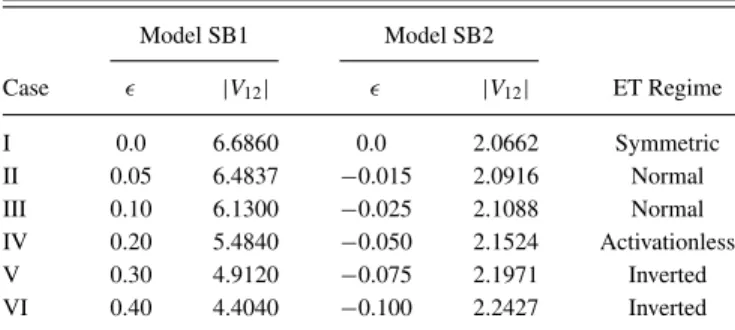
TABLE IV. Values of the asymmetry parameterconsidered in the system-bath representation, the corresponding thermodynamic driving force regimes, and the electronic coupling matrix element,V12.a
Model SB1 Model SB2 Case |V12| |V12| ET Regime I 0.0 6.6860 0.0 2.0662 Symmetric II 0.05 6.4837 −0.015 2.0916 Normal III 0.10 6.1300 −0.025 2.1088 Normal IV 0.20 5.4840 −0.050 2.1524 Activationless V 0.30 4.9120 −0.075 2.1971 Inverted VI 0.40 4.4040 −0.100 2.2427 Inverted aThe coupling|V
12|is given in units of a.u./107for Model SB1 and a.u./105for Model
SB2;is in atomic units.
the values ofconsidered for the system-bath representation are presented in TableIV.
The second term in the system potential energy function models the solvent and its interactions with the transferring electron: Ue−sol(q, s)=μstanh (φq)+ 1 2msω 2 ss2. (50)
The first term on the RHS of this equation describes the cou-pling of the electronic dipole of the redox system to the sol-vent dipole, and ωs is the effective frequency of the solvent
coordinate.
The harmonic oscillator bath potential in Eq.(49)has the same form as in Eq.(24):
UB(s,Q)= f j=1 ⎡ ⎣1 2Mω 2 j Qj − cjs Mωj2 2⎤ ⎦. (51) The bath exhibits Ohmic spectral density with cutoff fre-quencyωc,
J(ω)=ηωe−ω/ωc, (52)
where the dimensionless parameterηdetermines the strength of coupling between the system and the bath modes.52 The continuous spectral density is discretized into f oscillators with frequencies32 ωj = −ωclog j −0.5 f (53) and coupling constants
cj =ωj 2ηMωc f π 1/2 , (54) wherej =1. . . f.
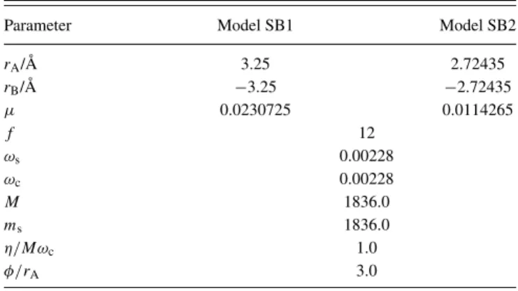
In the current paper, we use two sets of parameters for the system-bath representation. Model SB1 is constructed to reproduce the energy-scales of the atomistic representation, and Model SB2 uses parameters that are numerically less de-manding for the QUAPI calculations. The parameters for the models are given in TableV.
As indicated previously, the QUAPI method is imple-mented using a discrete representation for the diabatic states of the redox system (Eq. (23)). The system representation in the position basis described in Eq. (48) is therefore
TABLE V. Parameters for the system-bath representation of ET.a
Parameter Model SB1 Model SB2
rA/Å 3.25 2.72435 rB/Å −3.25 −2.72435 μ 0.0230725 0.0114265 f 12 ωs 0.00228 ωc 0.00228 M 1836.0 ms 1836.0 η/Mωc 1.0 φ/rA 3.0
aParameters given in atomic units, unless otherwise specified.
transformed to the electronic diabatic basis for the QUAPI calculations. The resulting diagonal matrix elements for the system potential energy are
V11(s)=a1s2+b1s+c1 (55)
and
V22(s)=a2s2+b2s+c2, (56)
and the constant off-diagonal elements V12 are reported in TableIV. The details of this transformation and the values of the coefficients in Eqs.(55)and(56)are given in AppendixB. IV. CALCULATION DETAILS
A. Atomistic representation
The atomistic system includes 430 SPC water molecules in a cubic simulation cell with periodic boundary conditions. The side-length of the cell isL = 23.46 Å. All calculations are performed at a temperature ofT = 300 K, and all pair-wise interactions are truncated at a distance of rcut = L/2.
Long-range electrostatics are treated by the force-shifting algorithm,80 where the Coulombic portion of each potential is multiplied by a damping function S(r), such that both the potential and its derivative smoothly vanish at r = rcut.
Specifically, S(r)= ⎧ ⎨ ⎩ 1− 2r rcut+ r2 rcut2 , r≤rcut 0, r > rcut . (57)
Force-shifting reduces the unphysical structuring of water near the cutoff radius,80 and it is found to have little effect on the solvent environment of the redox system.
1. RPMD
The atomistic RPMD simulations are implemented in the
DL_POLYmolecular dynamics package.81 In all simulations, the RPMD equations of motion are evolved using the velocity Verlet algorithm,82and the constraints in the rigid-body water model are implemented using the RATTLE algorithm.83The electron is quantized with n = 1024 ring-polymer beads. As in previous RPMD simulations, each timestep for the electron ring polymer involves separate coordinate updates due to forces arising from the physical potential and due
to exact evolution of the purely harmonic portion of the ring-polymer potential. The resulting integration algorithm is time-reversible and symplectic.
Several collective variables are used to characterize the ET reaction in the atomistic representation. The position of the electron is described by a ring-polymer progress variable, or a “bead-count” coordinate, defined as
fb(q(1), . . . ,q(n))= 1 n n α=1 1 2 tanhbqz(α)+1, (58) where b = 1.25 Å−1, and the metal ions are symmetrically
positioned on thez-axis. We also consider the solvent collec-tive variable U(Q)= − e 4π ε0 N k=1 qk |QD−Qk| − qk |QA−Qk| , (59)
whereqk∈ {qH,qO}is the charge on solvent atomk. This
sol-vent collective variable, which is familiar from earlier simula-tion studies of Marcus theory,76,84describes the energy differ-ence between the electronic diabatic states in the tight-binding approximation.
The RPMD rate in Eq.(3) is calculated from the prod-uct of the TST rate and the transmission coefficient. The TST rate described in Eq.(4)is obtained fromF(fb), the FE pro-file in the bead-count coordinate. This FE propro-file is calculated using umbrella sampling and the weighted histogram analysis method (WHAM), as described below.85,86
For each value of the asymmetry parameter , the fol-lowing umbrella sampling protocol is used. The region fb
= 0.06 − 0.94 is sampled with 22 trajectories that are har-monically restrained to uniformly spaced values of fb
us-ing a restraint force constant of 1.195 × 10⁴kcal/mol. Like-wise, the regionsfb = 0.945 − 1.0 andfb = 0.0 − 0.055
are each sampled with 11 uniformly spaced windows using a higher force constant of 1.195 × 10⁵ kcal/mol. The
re-gions offb = 0.986 − 0.991 andfb = 0.009 − 0.015 are each sampled with 5 uniformly spaced windows using a force constant of 1.195 × 10⁵kcal/mol. The equilibrium sampling
trajectories are performed using path-integral molecular dy-namics (PIMD) with a Parrinello-Rahman mass of 364.6 a.u., which allows for a timestep of 0.025 fs; this choice of mass does not affect the calculated FE profile or any other equi-librium ensemble average.39,87 Each sampling trajectory is run for at least 50 ps, and thermostatting is performed dur-ing the trajectory calculations by resampldur-ing the particle ve-locities from the Maxwell-Boltzmann (MB) distribution every 1.25 ps.
The transmission coefficient in Eq.(11)is calculated us-ing RPMD trajectories that are released from the dividus-ing surface at fb‡. For each value of , the dividing surface is chosen to coincide with the maximum along the FE pro-file,F(fb). The positions of the dividing surfaces are set to
fb‡ = (0.5,0.7,0.8,0.96,0.98,0.98,0.98) for the different -cases (I, II,. . ., VI) in Table III. Between 400 and 1200 trajectories are released for each value of. Each RPMD tra-jectory is evolved for 40 fs with a timestep of 5 × 10⁻⁵ fs
and with the initial velocities sampled from the MB distribu-tion. Initial configurations for the released RPMD trajectories
TABLE VI. ET reaction rates for the atomistic representation, obtained us-ing RPMD and Marcus theory.a
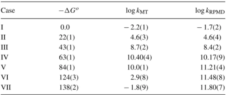
Case −Go logk MT logkRPMD I 0.0 −2.2(1) −1.7(2) II 22(1) 4.6(3) 4.6(4) III 43(1) 8.7(2) 8.4(2) IV 63(1) 10.40(4) 10.17(9) V 84(1) 10.0(1) 11.21(4) VI 124(3) 2.9(8) 11.48(8) VII 138(2) −1.8(9) 11.80(7)
aET rates are given in s−1, and the−G0are given in kcal/mol. The numbers in
paren-theses denote the statistical uncertainty in the last reported digit.
are selected every 100 fs from eight long, independent PIMD sampling trajectories that are constrained to the dividing sur-faceξ‡. These sampling trajectories are thermostatted by re-sampling the velocities every 200 fs, and the constraint to the dividing surface is enforced using the RATTLE algorithm.
Two-dimensional (2D) FE surfaces in the ring-polymer centroid coordinate and the solvent coordinate, F(¯z, U), are used for the analysis of the ET reaction mechanism. For a given value of , the 2D FE surface is constructed using PIMD sampling trajectories that are harmonically restrained in both ¯z and U coordinates. The ¯z coordinate is sam-pled using 43 uniformly spaced windows in the region of
−3.575 Å to+3.575 Å with a harmonic restraint force con-stant of 169.7 kcal/mol Å−2. To ensure adequate sampling of
ring-polymer configurations spanning both metal ions, we use four additional sampling trajectories that are harmonically re-strained to ¯z = ±2.7625 Å and ¯z = ±2.925 Å with a force constant of 452.5 kcal/mol Å−2. The solvent coordinate is
sampled with 15 uniformly spaced windows in the range of
−130 to+150 kcal/mol using a harmonic restraint force con-stant of 0.023 (kcal/mol)−1. Each sampling trajectory is run for at least 50 ps, with velocities resampled from the MB dis-tribution every 500 fs. We note that fb is a good progress
variable for ET throughout the entire regime of the thermo-dynamic driving forces, whereas the ring-polymer centroid is not. In the ET inverted regime, the centroid does not fully dis-tinguish between ring-polymer configurations in the reactant and product basins; no such difficulty is experienced in the calculations reported here.
2. Marcus theory
Marcus theory rates are calculated using Eqs. (37)
and(38). The driving force,−G0, is obtained fromF(U)
as the difference between the free energies of the reactant and product minima; these values are reported in Table VI. To the extent that the tight-binding approximation holds, the reorganization energy, λ, is identical for all , and we con-firm that this is very nearly the case in our calculations. For the case of symmetric ET ( = 0), the reorganization energy is calculated using λ = 4F(U)|U=0 and is found to be
69.7 ±0.7 kcal/mol.
The coupling matrix element in Eq.(37),|V12|, is calcu-lated as 2|V12| = E1 − E0, whereE0 andE1 are the two lowest eigenenergies of the electron in the potential of the isolated metal ions with = 0. These eigenenergies are
ob-tained with an iterative, block Lanczos scheme,88performed on a uniform grid of 64 × 64 × 64 points spanning the cu-bic simulation cell. The iterative Lanczos calculation employs 200 Krylov vectors and an exponential transform parameter of βL = 0.1. The block Lanczos refinement uses ten blocks of
five Krylov vectors. This yields a value for the tunnel split-ting of |V12| = 0.0403 kcal/mol (6.43 × 10⁻⁵ a.u.), which
is consistent with previous calculations.76 This value for the tunnel splitting was assumed to be insensitive to the presence of solvent, as has been previously demonstrated,89 and inde-pendent of the value of the asymmetry parameter. The valid-ity of this latter assumption is confirmed for the system-bath models (see TableIV).
B. System-bath representation
As in the atomistic representation, the calculations in the system-bath representation are performed atT = 300 K. The harmonic bath is discretized usingf = 12 modes.
1. RPMD
RPMD rates for the system-bath models are also cal-culated with the electron quantized using n = 1024 ring-polymer beads. For each value of , the FE profile, F(fb), is obtained from umbrella sampling along thefb coordinate. For both system-bath models, SB1 and SB2,F(fb) is sampled
with two sets of harmonically restrained PIMD trajectories. The region offb = 0.06 − 0.94 is sampled with 45
trajec-tories that are harmonically restrained to uniformly spaced values of fb using a force constant of 20 a.u. The regions
offb = 0.0 − 0.05 andfb = 0.095 − 1.00 are each
sam-pled with 51 uniformly spaced windows using a harmonic re-straint force constant of 3000 a.u. All sampling trajectories are performed using PIMD with the masses of the classical particles set to ms = M = 0.01 a.u; as before, the altered
masses in the PIMD sampling trajectories allow for larger timesteps while having no effect on calculated ensemble av-erages. Each sampling trajectory is run for at least 12.09 ps, the PIMD timestep is 2.42 × 10⁻⁴fs, and thermostatting is
performed by resampling velocities from the MB distribution every 2.42 fs. The FE profiles are constructed from the sam-pling trajectories using WHAM.
For each value of, the transmission coefficient in Model SB1 is calculated from 2400 RPMD trajectories released from the dividing surface and evolved for 121 fs with the timestep of 1.21 × 10⁻⁴ fs. The position of the dividing surface isfb‡ = (0.5,0.385,0.2345,0.014,0.014,0.014) for the -cases (I, II, . . ., VI). In Model SB2, 1600 RPMD tra-jectories are released at each value of ; each trajectory is evolved for 121 fs using a timestep of 2.42 × 10⁻⁴ fs; and
the dividing surface is located atfb‡=(0.5, 0.65, 0.75, 0.986, 0.986, 0.986) for-cases (I, II,. . ., VI). Initial configurations for the released RPMD trajectories are sampled every 14.5 fs from eight long, independent PIMD sampling trajectories that are constrained to the dividing surface. The velocities of the PIMD sampling trajectories are resampled every 48.4 fs from the MB distribution. The dividing surface constraint is imple-mented using the RATTLE algorithm.
We note that RPMD results can be affected by coupling of fictitious internal ring-polymer modes to physical frequen-cies in the system.90 We thus performed test calculations of the ET rate in these and similar systems using partially adiabatic centroid molecular dynamics (PACMD).90,91 The PACMD calculations revealed no significant changes from the RPMD results, confirming that this issue does not impact our conclusions.
2. Marcus theory
For the calculation of Marcus theory rates, the reorga-nization energy and the thermodynamic driving force for each value of epsilon are obtained analytically from the diabatic states for the donor and the acceptor, V11(s) and
V22(s). For Model SB1, we obtain a solvent reorganization
energy ofλ = 68.9 kcal/mol, and for Model SB2, we obtain λ = 17.0 kcal/mol. The values of|V12|for both system-bath models are given in TableIV.
3. Semiclassical instanton theory
For the SB models, contributions from the linearly cou-pled harmonic bath can be factorized and cancelled from the RHS of Eq. (12), yielding expressions that depend only on the electron ring-polymer coordinates and the single classi-cal solvent coordinate,s. Calculation ofkSCI then consists of (i) determination of saddle-point configurations for the clas-sical action, A({q(α)};s), on a numerical grid in the solvent
coordinates, (ii) evaluation of the steepest-descent approxi-mation for In(s) at each point on the solvent grid, and (iii) integration over the solvent coordinate in Eq. (19) via nu-merical quadrature. The reactant partition function, Qr, was similarly obtained by evaluatingIn(s) via steepest-decent ex-pansion around the minimum-action configuration in the reac-tant basin. All calculations were performed usingn = 2048 beads for the electron ring polymer.
For Model SB1, the grid in the solvent coordinates con-sists of 200 uniformly spaced points in the range of −4 to 4 a.u.; for Model SB2, this grid consists of 150 uniformly spaced points in the range of−3 to 3 a.u. At each value ofs, the saddle-point configuration on the surfaceA({q(α)};s)
cor-responds to the maximum along the path of minimum action that connects the reactant and product basins. This path of minimum action is obtained using the string method,92 with the path discretized into L = 1000 equidistant slices and with minimization performed using Euler integration and a timestep of 2.4 × 10⁻³ fs. Initial convergence of the path is
achieved when this minimization results in a change of less than 5.3 × 10⁻⁸ Å in each degree of freedom. The path is
then iteratively refined in the vicinity of the saddle point: a 20-slice sub-section of the path about the saddle point is ex-tracted, the number of slices used to describe the path is dou-bled, and the sub-section of the path is re-minimized with its endpoints fixed. Iterative refinement of the path is complete when the slice of maximum action (i.e., the saddle point con-figuration) satisfies Eq.(16)to within 10−5a.u.
4. QUAPI
The QUAPI calculation for Model SB2 requires con-struction of the short-time system propagator followed by two independent Monte Carlo (MC) simulations to evaluate the flux-flux correlation function in Eq.(29).
The complex-time propagator in Eq. (33) is calculated using eigenvalues and eigenfunctions obtained from a 2D dis-crete variable representation (DVR) grid calculation93 in the solvent coordinate, s, and the electronic state variable, σ. The DVR Hamiltonian is diagonalized on a grid of 40 uni-formly spaced points over a range of−4 to+4 a.u. insand σ = 1,2. The number of eigenvalues and eigenvectors used in these calculations (M0in Eq.(33)) ranges from 30 to 50 for
the values ofconsidered in this study.
The flux-flux correlation function in Eq.(29)is obtained from standard path-integral Monte Carlo (PIMC) sampling performed on the 2D DVR grid. In a first PIMC simulation, the correlation function is obtained using
CFF(t)=Dρsgn{Re [I1(s,σ;tc)−I2(s,σ;tc)
+I3(s,σ;tc)−I4(s,σ;tc)]}ρ(s,σ;tc), (60)
where importance sampling is performed using the distribution
ρ(s, σ;tc)=Abs{Re [I1s(σ;tc)−I2(s,σ;tc)
+ I3(s,σ;tc)−I4(s,σ;tc)]}, (61)
and the function Ii(s,σ;tc) is defined in Eq. (31).
Conver-gence is achieved with 108MC steps. The normalization
con-stant,Dρ, is obtained from a second, independent PIMC sim-ulation, using Dρ=D ρ(s,σ;tc) (s,σ;tc) (s,σ;tc) . (62)
Here, importance sampling is performed on the distribution (s,σ;tc)= 2N+2 k=N+3 |σk, sk|eiHSt ∗ c/¯|σ k−1, sk−1| × N+1 k=2 |σk, sk|e−iHStc/¯|σk−1, sk−1|, (63) where σ1 = 2, σN+1 = 2, σN+2 = 1, and σ2N+2 = 1.
Convergence is achieved with 106MC steps, and the normal-ization constant D is obtained by direct matrix multiplica-tion. A maximum ofN = 4 path beads are required to con-verge the flux-flux correlation function over a timescale of 25 fs; no significant changes are observed between calcula-tions performed usingN = 4 andN = 8.
The reactant partition function is obtained from a single PIMC calculation using the expression
Qr =Tr[e−βHP1], (64) whereP1 = |11|is the projection operator for the reactant
electronic state.
The QUAPI calculations for case IV are performed using a larger value for the coupling between the solvent coordi-nate and the bath modes,η/Mωc = 30. This change leads to
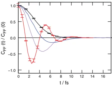
lower-amplitude oscillations in the flux-flux correlation func-tion and improved numerical convergence of the ET rate cal-culation. Other features of the flux-flux correlation function, including the timescales for the real-time oscillations and the decorrelation time, are unchanged. The invariance of these features suggests that the parameters used in the current study correspond to the regime in which the ET reaction rate is inde-pendent of the solvent-bath coupling.65,94RPMD rate calcu-lations performed using different values forη/Mωcalso sup-port this conclusion.
V. RESULTS
A. Atomistic simulations
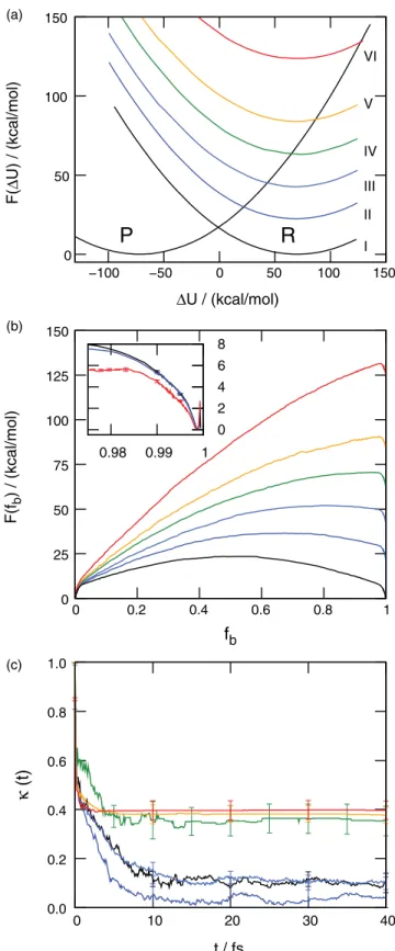
The atomistic representation for ET (Fig. 1) is inves-tigated using direct RPMD simulations and the Marcus rate theory. For each case of the thermodynamic driving force, Fig. 2(a) presents FE profiles for the reactant and product diabatic electronic states as a function of the sol-vent collective variable, U(Q) (Eq. (59)). The FE pro-files are obtained by reducing the corresponding 2D surfaces, F(fb, U), where the reactant and product diabats are
associ-ated with ring-polymer configurations for whichfb > 0.995
and fb < 0.005, respectively. The results in Fig. 2(a) are
graphically identical to those obtained using the tight-binding approximation, and the FE profiles exhibit the anticipated parabolic form, although no assumptions regarding the lin-ear response of the solvent have been made.76,84 These data, in combination with the calculated tunnel splitting for the transferring electron, are used to calculate the Marcus rates in TableVI.
Figure 2(b)presents the corresponding FE profiles as a function of the bead-count coordinate, fb (Eq. (58)). These
profiles are used in the statistical component of the RPMD rate calculation (Eqs.(3)and(4)). As is seen from the inset, all of the profiles behave similarly in the vicinity offb ≈ 1.
The steep rise in the FE profile between 0.980 and 0.999 is as-sociated with the formation of “kink-pair” configurations, in which the ring polymer spans both redox sites;25,95,96a typi-cal kink-pair configuration is illustrated in Fig.1(a).
The dynamical component of the RPMD rate calcula-tion (Eq. (11)) is obtained from the long-time plateau46 of the RPMD transmission coefficient shown in Fig.2(c). Each transmission coefficient is calculated with respect to a divid-ing surface at a fixed value offb, as is described in Sec.IV A.
Plateau values in the range of 0.1–0.4 indicate modest recross-ing of the RPMD trajectories through these surfaces. For cases in which the thermodynamic driving force corresponds to ET in the normal and activationless regimes, Fig.2(c)illustrates that the RPMD trajectories commit to the reactant or product basins within 10–20 fs, the timescale for local solvent mo-tion between libramo-tional rebounds. At thermodynamic driving forces corresponding to the inverted regime, the transmission coefficient plateaus on faster timescales than those involving the rigid solvent molecules.
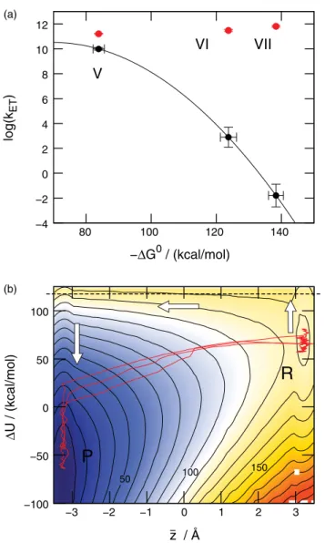
Figure 3(a)presents a direct comparison of the RPMD and Marcus theory rates throughout the normal and activa-tionless regime for ET in the atomistic representation. The RPMD rates, which are also reported in Table VI,
0 50 100 150 −100 −50 0 50 100 150 F( Δ U) / (kcal/mol) ΔU / (kcal/mol) I II III IV V VI
R
P
0 25 50 75 100 125 150 0 0.2 0.4 0.6 0.8 1 F(f b ) / (kcal/mol) fb 0.98 0.99 1 0 2 4 6 8 0.0 0.2 0.4 0.6 0.8 1.0 0 10 20 30 40 κ (t) t / fs (c) (b) (a)FIG. 2. (a) FE profiles,F(U), for the reactant (colored, at right) and prod-uct (left) diabatic electronic states as a function of the solvent collective vari-able in the atomistic representation. The various cases of the thermodynamic driving force for the ET reaction are labeled; see TablesIIIandVIfor details. For each case, the FE profiles are vertically shifted to align the minima of the product basin. (b) The corresponding FE profiles as a function of the bead-count coordinate,F(fb). In the main panel, the profiles are vertically shifted
to align the product basin; in the inset, the profiles are vertically shifted to align the reactant basin. (c) The corresponding RPMD transmission coeffi-cients for the ET reaction,κ(t). In panels (b) and (c), the curves retain the same color scheme introduced in panel (a).
tively agree with the Marcus theory results over 12 orders of magnitude in the ET reaction rate. Unlike the Marcus rates, which are based on a TST description for the reaction, the calculated RPMD rates are independent of any a priori as-sumptions about the ET reaction mechanism.
Figures 3(b)and3(c)illustrate the ET reaction mecha-nism that is predicted from the RPMD simulations. Repre-sentative RPMD trajectories are projected onto the (¯z, U) plane, where ¯zis the component of the ring-polymer centroid that lies along the axis of the metal ions in the system; also shown are FE profiles for the system in these collective vari-ables. For symmetric ET (Case I), Fig. 3(b)reveals that the RPMD trajectories involve three distinct steps that will be fa-miliar from the Marcus rate theory: (i) solvent fluctuation to a configuration for which the reactant and product diabats are nearly degenerate (indicated by the dashed line), (ii) forma-tion of a kink-pair in the ring-polymer configuraforma-tion and rapid transfer of the electron from one redox site to the other, and (iii) relaxation of the solvent coordinate in the product basin following the ET event. For ET approaching the activationless regime (Case IV), Fig.3(c)shows that the latter two steps in the mechanism remain, but only a small initial solvent fluctu-ation is needed to reach solvent configurfluctu-ations for which the electronic diabats are degenerate.
To understand the connection between RPMD and the Marcus theory rate expression, we note that Eq. (37) in-cludes two key terms – an Arrhenius-type contribution that is associated with the free energy of solvent reorganization to bring reactant and product diabats into degeneracy and a prefactor that depends on the coupling between the diabatic states. RPMD captures the solvent reorganization energetics because the path-integral-based method preserves exact quan-tum statistics.39,87The RPMD rate also correctly accounts for the tunneling contribution to the ET reaction rate, which can likewise be attributed to the path-integral basis of the method; the tunnel splitting for the electron between degenerate redox sites is analytically related to the reversible work for forming a kink-pair in the ring-polymer configuration.25,89,96 Given that the ensemble of reactive RPMD trajectories exhibits the dual rare events of solvent reorganization and kink-pair for-mation, and given that the FE barriers associated with these two steps are analytically related to the key terms in the Mar-cus rate expression, it is reasonable that Fig.3(a)finds good agreement between RMPD and Marcus theory. The RPMD method succeeds in the normal and activationless regimes be-cause it captures the correct physics of the ET reaction.
Figure 4 demonstrates that the success of the RPMD method does not extend into the inverted regime for ET, with both the RPMD rates and the reaction mechanism deviating from the predictions of Marcus theory. In Fig.4(a), the RPMD rates are seen to be only weakly dependent on the increasing driving force, rather than exhibiting the character-istic turnover in this inverted regime. The RPMD trajectories also deviate from the reaction mechanism that is assumed in the Marcus TST, as is seen in Fig.4(b). The reactive trajec-tories exhibit kink-pair formation directly from solvent con-figurations that are characteristic of the reactant basin; the ex-pected solvent reorganization to configurations for which the
−4 −2 0 2 4 6 8 10 0 20 40 60
log(k
ET)
−
Δ
G
0/ (kcal/mol)
I
II
III
IV
−100 −50 0 50 100Δ
U / (kcal/mol)
10 30 50 70 (b) (a)R
P
−3 −2 −1 0 1 2 3 −z / Å
−100 −50 0 50 100Δ
U / (kcal/mol)
10 30 50 70 90 110R
P
(c)FIG. 3. (a) ET reaction rates for the atomistic representation in the normal and activationless regimes, computed using RPMD (red) and Marcus theory (black). The various cases for the thermodynamic driving force are labeled. (b) Representative trajectories (red) from the ensemble of reactive RPMD tra-jectories for symmetric ET (Case I). The tratra-jectories are plotted as a function of the ring-polymer centroid, ¯z, and the solvent collective variable,U. The FE profile in these collective variables is also presented, with contour lines indicating FE increments of 10 kcal/mol. (c) Representative RPMD trajecto-ries for activationless ET (Case IV) and the corresponding FE profile. The white arrows in panels (b) and (c) indicate the solvent reorganization mech-anism for ET that is anticipated in the Marcus rate theory, and the dashed lines indicate values ofUat which the reactant and product diabats cross in Fig.2(a).
−4 −2 0 2 4 6 8 10 12 80 100 120 140 log(k ET ) −ΔG0 / (kcal/mol)
V
VI VII
−3 −2 −1 0 1 2 3 − z / Å −100 −50 0 50 100 Δ U / (kcal/mol) (b) (a)R
P
50 100 150FIG. 4. (a) ET reaction rates for the atomistic representation in the inverted regime, computed using RPMD (red) and Marcus theory (black). The vari-ous cases for the thermodynamic driving force are labeled. (b) Representa-tive trajectories (red) from the ensemble of reacRepresenta-tive RPMD trajectories for inverted ET (Case VI). The trajectories are plotted as a function of the ring-polymer centroid, ¯z, and the solvent collective variable,U. The FE profile in these collective variables is also presented, with contour lines indicating FE increments of 10 kcal/mol. The white arrows indicate the solvent reorga-nization mechanism for ET that is anticipated in the Marcus rate theory, and the dashed line indicates the value ofUat which the reactant and product diabats cross in Fig.2(a).
electronic diabats are degenerate (indicated by the dashed line in the figure) is not observed.
To further explore the successes and failures of RPMD in these various regimes for ET, we compare the method with semiclassical instanton theory and exact quantum dynamics in the following section.
B. System-bath simulations
In this section, we employ system-bath representations for ET to allow for the comparison of RPMD with other simu-lation techniques, including semiclassical instanton and exact quantum dynamics methods.
Figure 5(a) and TableVII present a comparison of the RPMD and Marcus rates for Model SB1, which is parameter-ized to match the energy-scales for the atomistic
representa-−8 −6 −4 −2 0 2 4 6 8 0 50 100 150 log(k ET ) −ΔG0 / (kcal/mol) I II III IV V VI 0 50 100 150 200 −2 −1 0 1 2 3 E / kcal/mol s / Å I II III IV V VI (b) (a)
FIG. 5. (a) ET reaction rates for Model SB1, computed using RPMD (red), Marcus theory (black), and SCI theory (blue). (b) FE profiles,F(U), for the reactant (colored, at right) and product (left) diabatic electronic states as a function of the solvent coordinate,s. The various cases of the thermody-namic driving force for the ET reaction are labeled; see TableIVfor details. The arrow indicates the value of the solvent coordinate that maximizesIn(s),
which corresponds to the dominant contribution to the SCI rate in Eq.(19).
tion (Sec. III B). As before, the RPMD method reproduces the Marcus rates throughout the normal and activationless regimes, while failing to predict the turnover of the ET rate in the inverted regime. Analysis of the RPMD reactive trajecto-ries in this system reveals mechanisms that are entirely anal-ogous to those observed in Figs. 3(b),3(c), and4(b)for the atomistic system. Specifically, for the normal and activation-less regimes, the RPMD trajectories exhibit solvent reorga-nization to configurations for which the electronic diabats are degenerate, followed by rapid transfer of the electron between redox sites; and for the inverted regime, RPMD predicts ET without prior solvent reorganization. These data confirm that Model SB1 exhibits the same essential physics as the atom-istic representation.
ET rates from the steepest-descent SCI theory (Eq.(19)) are also included in Fig. 5(a) and Table VII. Throughout the full range of thermodynamic driving forces, the instanton method tracks the RPMD results, including deviation from the Marcus predictions in the inverted regime. As is shown in TableVII,α-correction of the RMPD rates (Eq.(22),
assum-TABLE VII. ET reaction rates for Model SB1, obtained using RPMD, Mar-cus theory, and SCI theory.a
Case −G0 logk
MT logkRPMD logkSCI logαkRPMD
I 0.0 −6.0 −6.55(4) −7.9 −7.3 II 18.5 −0.2 −0.33(3) −1.9 −0.9 III 36.9 3.7 3.52(8) 2.4 2.8 IV 73.9 6.3 6.19(5) 5.6 5.4 V 110.9 1.6 6.44(1) 5.8 5.8 VI 148.0 −10.4 6.69(3) 5.9 5.9
aET rates are given in s−1, and the−G0are given in kcal/mol.
ing κo ≈ 1) further improves their agreement with the SCI
rates. These results underscore that the failure of RPMD does not arise from a breakdown in its formal connection with SCI theory;37 instead, the comparison suggests that both RPMD and the SCI theory share the same underlying flaw in the in-verted regime.
The mechanistic predictions from SCI theory also show similarities with the RPMD results. Figure5(b)presents the Marcus parabolas for the electronic diabats of Model SB1 as a function of the solvent coordinate, s. Also shown are the solvent configurations that correspond to the SCI predictions for the ET transition state. For each value of the thermody-namic driving force, the arrow in the figure indicates the sol-vent configuration that maximizes In(s), which corresponds to the largest contribution to the rate in Eq.(19). For the nor-mal and activationless regimes, SCI theory correctly predicts an ET transition state at the crossing of the electronic diabats. However, in the inverted regime, the SCI transition state is instead located at the minimum of the reactant basin. These mechanistic results from SCI theory are consistent with the observed pathways for the RPMD trajectories, which suggests that in the inverted regime, both RPMD and SCI theory over-estimate the degree of ET from solvent configurations in the reactant basin.
To further illustrate this issue, we present SCI rate cal-culations for deep tunneling in a 1D asymmetric double well. Table VIII presents ET reaction rates calculated on the potential energy surfaceUe-M(q) (Eq.(49)), with
param-eters from Model SB1. Although this is a non-dissipative 1D system, the SCI rate is still well-defined, and it is reported as a function of the potential energy asymmetry. The rates plateau to a finite value with increasing asymme-try, which is consistent with rates for deep tunneling between
TABLE VIII. ET reaction rates for a 1D asymmetric double well, obtained using SCI theory.a
E logkSCI 0.0 0.0 −11.0 0.05 0.02940 −10.9 0.10 0.05884 −10.8 0.20 0.11776 −10.6 0.30 0.17676 −10.3 0.40 0.23584 −10.3
aThe golden rule for the symmetric case yields logk = −11.55.Eis the
differ-ence between the two lowest eigenenergies for the system. All quantities are reported in atomic units. −8 −6 −4 −2 0 2 4 6 8 0 50 100 150 log(k ET ) −ΔG0 / (kcal/mol)
I
II
III
IV
V
VI
FIG. 6. The ET rates for Model SB1 corresponding to a Marcus-like mech-anism (black) and the “direct” mechmech-anism in Eq.(66)(red). SCI rates (blue) correspond to the kinetically favorable mechanism in all regimes. See text for details.
a bound state and a continuum.98–100However, this behavior is qualitatively incorrect for tunneling rates between bound states, which should vanish for non-degenerate states in ac-cord with Fermi’s Golden Rule.101We conclude that SCI the-ory, as well as the closely related RPMD method, significantly overestimate the tunneling probability between asymmetric bound states, leading to an incorrect ET mechanism and over-estimation of the reaction rate in the inverted regime.
The results for the simple double-well system can be used to deduce a more general argument for the applicability of the RPMD and SCI calculations in ET problems. TableVIII, combined with the condition of detailed balance for the ther-mal reaction rate, indicates that the SCI rate for transfer in an asymmetric double-well system is approximately
k≈2π
¯ |V12|
2min(1, e−βE
). (65)
For the Marcus-type ET mechanism in which electron tunnel-ing is gated via solvent reorganization that symmetrizes the double-well system, Eq.(65)leads to the TST rate in Eq.(37). However, for an unphysical “direct” ET mechanism in which electron tunneling proceeds from solvent configurations in the reactant basin (i.e., without prior solvent reorganization), Eq. (65)leads to the following TST expression for the ET rate: kdirect= 2π ¯ |V12| 2 β 4π λ 1/2 min(1, e−β(λ+G0)). (66) Figure6presents the ET reaction rates for Model SB1, assum-ing either the Marcus-type mechanism (Eq.(37), black) or the direct mechanism (Eq. (66), red). Also plotted are the rates calculated using SCI theory (Eq.(19), blue). Throughout the normal and activationless regimes, the rate for the Marcus-type mechanism dominates; in the inverted regime, the rate for the direct mechanism dominates; and the results from SCI theory closely track the larger of these two rates. It is clear that SCI theory (as well as RPMD) features a competition between the correct, Marcus-type mechanism for ET and the