Robust Subspace Clustering
Mahdi Soltanolkotabi∗, Ehsan Elhamifar† and Emmanuel J. Cand`es‡
January 2013
Abstract
Subspace clustering refers to the task of finding a multi-subspace representation that best fits a collection of points taken from a high-dimensional space. This paper introduces an algorithm inspired by sparse subspace clustering (SSC) [18] to cluster noisy data, and develops some novel theory demonstrating its correctness. In particular, the theory uses ideas from geometric functional analysis to show that the algorithm can accurately recover the underlying subspaces under minimal requirements on their orientation, and on the number of samples per subspace. Synthetic as well as real data experiments complement our theoretical study, illustrating our approach and demonstrating its effectiveness.
Keywords. Subspace clustering, spectral clustering, LASSO, Dantzig selector, `1 minimiza-tion, true and false discoveries, geometric functional analysis, nonasymptotic random matrix theory.
1
Introduction
1.1 Motivation
In many problems across science and engineering, a fundamental step is to find a lower dimensional subspace which best fits a collection of points taken from a high-dimensional space; this is classically achieved via Principal Component Analysis (PCA). Such a procedure makes perfect sense as long as the data points are distributed around a lower dimensional subspace, or expressed differently, as long as the data matrix with points as column vectors has approximately low rank. A more general model might sometimes be useful when the data come from a mixture model in which points do not lie around a single lower-dimensional subspace but rather around a union of subspaces. For instance, consider an experiment in which gene expression data are gathered on many cancer cell lines with unknown subsets belonging to different tumor types. One can imagine that the expressions from each cancer type may span a distinct lower dimensional subspace. If the cancer labels were known in advance, one would apply PCA separately to each group but we here consider the case where the observations are unlabeled. Finding the components of the mixture and assigning each point to a fitted subspace is called subspace clustering. Even when the mixture model holds, the full data matrix may not have low rank at all, a situation which is very different from that where PCA is applicable.
∗Department of Electrical Engineering, Stanford University, Stanford CA
†Department of Electrical Engineering and Computer Science, University of California, Berkeley, Berkeley CA ‡Departments of Mathematics and of Statistics, Stanford University, Stanford CA
In recent years, numerous algorithms have been developed for subspace clustering and applied to various problems in computer vision/machine learning [47] and data mining [37]. At the time of this writing, subspace clustering techniques are certainly gaining momentum as they begin to be used in fields as diverse as identification and classification of diseases [33], network topology inference [20], security and privacy in recommender systems [51], system identification [3], hyper-spectral imaging [17], identification of switched linear systems [31,35], and music analysis [25] to name just a few. In spite of all these interesting works, tractable subspace clustering algorithms either lack a theoretical justification, or are guaranteed to work under restrictive conditions rarely met in practice. (We note that although novel and often efficient clustering techniques come about all the time, there seems to be very little theory about clustering in general.) Furthermore, proposed algorithms are not always computationally tractable. Thus, one important issue is whether tractable algorithms that can (provably) work in less than ideal situations—that is, under severe noise conditions and relatively few samples per subspace—exist.
Elhamifar and Vidal [18] have introduced an approach to subspace clustering, which relies on ideas from the sparsity and compressed sensing literature, please see also the longer version [19] which was submitted while this manuscript was under preparation. Sparse subspace clustering
(SSC) [18,19] is computationally efficient since it amounts to solving a sequence of `1 minimiza-tion problems and is, therefore, tractable. Now the methodology in [18] is mainly geared towards noiseless situations where the points lie exactly on lower dimensional planes, and theoretical per-formance guarantees in such circumstances are given under restrictive assumptions. Continuing on this line of work, [41] showed that good theoretical performance could be achieved under broad circumstances. However, the model supporting the theory in [41] is still noise free.
This paper considers the subspace clustering problem in the presence of noise. We introduce a tractable clustering algorithm, which is a natural extension of SSC, and develop rigorous theory about its performance. In a nutshell, we propose a statistical mixture model to represent data lying near a union of subspaces, and prove that in this model, the algorithm is effective as long as there are sufficiently many samples from each subspace and that the subspaces are not too close to each other. In this theory, the performance of the algorithm is explained in terms of interpretable and intuitive parameters such as (1) the values of the principal angles between subspaces, (2) the number of points per subspace, (3) the noise level and so on. In terms of these parameters, our theoretical results indicate that the performance of the algorithm is in some sense near the limit of what can be achieved by any algorithm, regardless of tractability.
1.2 Problem formulation and model
We assume we are given data points lying near a union of unknown linear subspaces; there are
L subspaces S1, S2, . . . , SL of Rn of dimensions d1, d2, . . . , dL. These together with their number
are completely unknown to us. We are given a point set Y ⊂Rn of cardinality N, which may be
partitioned as Y = Y1∪ Y2∪. . .∪ YL; for each `∈ {1, . . . , L}, Y` is a collection of N` vectors that
are ‘close’ to subspaceS`. The goal is to approximate the underlying subspaces using the point set Y. One approach is first to assign each data point to a cluster, and then estimate the subspaces representing each of the groups with PCA.
Our statistical model assumes that each pointy∈ Y is of the form
y=x+z, (1.1)
suppose that the inverse signal-to-noise ratio (SNR) defined as E∥z∥22/∥x∥2`
2 is bounded above.
Each observation is thus the superposition of a noiseless sample taken from one of the subspaces and of a stochastic perturbation whose Euclidean norm is aboutσ times the signal strength so that
E∥z∥2
`2 =σ
2∥x∥2
`2. All the way through, we assume that σ<σ⋆, and max
` d`<c0
n
(logN)2, (1.2)
whereσ⋆<1 andc0 are fixed numerical constants. The second assumption is here to avoid unnec-essarily complicated expressions later on. While more substantial, the first is not too restrictive since it just says that the signal x and the noise z may have about the same magnitude. (With an arbitrary perturbation of Euclidean norm equal to two, one can move from any pointxon the unit sphere to just about any other point.)
This is arguably the simplest model providing a good starting point for a theoretical investiga-tion. For the noiseless samples x, we consider the intuitivesemi-random model introduced in [41], which assumes that the subspaces are fixed with points distributed uniformly at random on each subspace. One can think of this as a mixture model where each component in the mixture is a lower dimensional subspace. (One can extend the methods to affine subspace clustering as briefly explained in Section 2.)
1.3 What makes clustering hard?
Two important parameters fundamentally affect the performance of subspace clustering algorithms: (1) the distance between subspaces and (2) the number of samples we have on each subspace.
1.3.1 Distance/affinity between subspaces
Intuitively, any subspace clustering algorithm operating on noisy data will have difficulty segmenting observations when the subspaces are close to each other. We of course need to quantify closeness, and the following definition captures a notion of distance or similarity/affinity between subspaces.
Definition 1.1 The principal anglesθ(1), . . . , θ(d∧d′)between two subspacesSandS′of dimensions
dand d′, are recursively defined by
cos(θ(i)) =max u∈S maxv∈S′ uTv ∥u∥` 2∥v∥`2 ∶= uTi vi ∥ui∥`2∥vi∥`2
with the orthogonality constraints uTuj =0, vTvj =0, j=1, . . . , i−1.
Alternatively, if the columns of U and V are orthobases for S and S′, then the cosine of the principal angles are the singular values ofUTV.
Definition 1.2 The normalized affinity between two subspaces is defined by
aff(S, S′) =
√
cos2θ(1)+. . .+cos2θ(d∧d′)
The affinity is a measure of correlation between subspaces. It is low when the principal angles are nearly right angles (it vanishes when the two subspaces are orthogonal) and high when the principal angles are small (it takes on its maximum value equal to one when one subspace is contained in the other). Hence, when the affinity is high, clustering is hard whereas it becomes easier as the affinity decreases. Ideally, we would like our algorithm to be able to handle higher affinity values—as close as possible to the maximum possible value.
There are other ways of measuring the affinity between subspaces; for instance, by taking the cosine of the first principal angle. We prefer the definition above as it offers the flexibility of allowing for some principal angles to be small or zero. As an example, suppose we have a pair of subspaces with a nontrivial intersection. Then ∣cosθ(1)∣ = 1 regardless of the dimension of the intersection whereas the value of the affinity would depend upon this dimension.
1.3.2 Sampling density
Another important factor affecting the performance of subspace clustering algorithms has to do with the distribution of points on each subspace. In the model we study here, this essentially reduces to the number of points we have on each subspace.1
Definition 1.3 The sampling density ρ of a subspace is defined as the number of samples on that subspace per dimension. In our multi-subspace model the density of S` is, therefore, ρ`=N`/d`.2
With noisy data, one expects the clustering problem to become easier as the sampling density increases. Obviously, if the sampling density of a subspaceSis smaller than one, then any algorithm will fail in identifying that subspace correctly as there are not sufficiently many points to identify all the directions spanned by S. Hence, we would like a clustering algorithm to be able to operate at values of the sampling density as low as possible, i.e. as close to one as possible.
2
Robust subspace clustering: methods and concepts
This section introduces our methodology through heuristic arguments confirmed by numerical ex-periments. Section 3 presents theoretical guarantees showing that the entire approach is math-ematically valid. From now on, we arrange the N observed data points as columns of a matrix
Y = [y1, . . . ,yN] ∈Rn×N. With obvious notation,Y =X+Z.
2.1 The normalized model
In practice, one may want to normalize the columns of the data matrix so that for alli,∥yi∥`2 =1.
Since with our SNR assumption, we have ∥y∥`2 ≈ ∥x∥`2
√
1+σ2 before normalization, then after normalization:
y≈ √ 1
1+σ2(x+z),
wherex is unit-normed, andz has i.i.d. random Gaussian entries with variance σ2/n.
1
In a general deterministic model where the points have arbitrary orientations on each subspace, we can imagine that the clustering problem becomes harder as the points align along an even lower dimensional structure.
2Throughout, we take ρ
`≤ed`/2. Our results hold for all other values by substituting ρ` withρ`∧ed`/2 in all the
For ease of presentation, we work—in this section and in the proofs—with a model y=x+z
in which∥x∥`2 =1 instead of ∥y∥`2 =1 (the numerical Section 6 is the exception). The normalized
model with∥x∥`2 =1 and z i.i.d.N (0, σ
2/n) is nearly the same as before. In particular, all of our methods and theoretical results in Section 3 hold with both models in which either ∥x∥`2 = 1 or
∥y∥`2 =1.
2.2 The SSC scheme
We describe the approach in [18], which follows a three-step procedure:
I Compute an affinity matrix encoding similarities between sample pairs as to construct a weighted graph W.
II Construct clusters by applying spectral clustering techniques (e.g. [34]) toW. III Apply PCA to each of the clusters.
The novelty in [18] concerns step I, the construction of the affinity matrix. This work is mainly concerned with the noiseless situation in whichY =X and the idea is then to express each column
xi of X as a sparse linear combination of all the other columns. The reason is that under any
reasonable condition, one expects that the sparsest representation ofxi would only select vectors
from the subspace in which xi happens to lie in. Applying the`1 norm as the convex surrogate of sparsity leads to the following sequence of optimization problems
min
β∈RN ∥β∥`1 subject to xi =Xβ and βi=0. (2.1)
Here, βi denotes the ith element of β and the constraint βi =0 removes the trivial solution that
decomposes a point as a linear combination of itself. Collecting the outcome of theseN optimization problems as columns of a matrix B, [18] sets the similarity matrix to beW = ∣B∣ + ∣B∣T.3 (This
algorithm clusters linear subspaces but can also cluster affine subspaces by adding the constraint
βT1=1 to (2.1).)
The issue here is that we only have access to the noisy data Y: this makes the problem challenging, as unlike conventional sparse recovery problems where only the response vector xi is
corrupted, here both the covariates (columns of X) and the response vector are corrupted. In particular, it may not be advisable to use (2.1) with yi and Y in place of xi and X as, strictly
speaking, sparse representations no longer exist. Observe that the expression xi = Xβ can be
rewritten as yi =Y β+ (zi−Zβ). Viewing (zi−Zβ) as a perturbation, it is natural to use ideas
from sparse regression to obtain an estimate ˆβ, which is then used to construct the similarity matrix. In this paper, we follow the same three-step procedure and shall focus on the first step in Algorithm 1; that is, on the construction of reliable similarity measures between pairs of points. Since we have noisy data, we shall not use (2.1) here. Also, we add denoising to Step III, check the output of Algorithm 1.
2.3 Performance metrics for similarity measures
Given the general structure of the method, we are interested in sparse regression techniques, which tend to select points in the same clusters (share the same underlying subspace) over those that do
3
Algorithm 1 Robust SSC procedure
Input: A data set Y arranged as columns ofY ∈Rn×N.
1. For each i∈ {1, . . . , N}, produce a sparse coefficient sequence ˆβ by regressing the ith vector
yi onto the other columns ofY. Collect these as columns of a matrixB.
2. Form the similarity graph G with nodes representing the N data points and edge weights given by W = ∣B∣ + ∣B∣T.
3. Sort the eigenvalues δ1 ≥δ2 ≥. . .≥δN of the normalized Laplacian of Gin descending order,
and set
ˆ
L=N−arg max
i=1,...,N−1 (
δi−δi+1).
4. Apply a spectral clustering technique to the similarity graph using ˆLas the estimated number of clusters to obtain the partition Y1, . . . ,YLˆ.
5. Use PCA to find the best subspace fits ({S`}L1) to each of the partitions ({Y`}L1) and denoise
Y as to obtain clean data points ˆX.
Output: Subspaces{S`}L1 and cleaned data points ˆX.
not share this property. Expressed differently, the hope is that whenever Bij ≠0,yi and yj belong
to the same subspace. We introduce metrics to quantify performance.
Definition 2.1 (False discoveries) Fix i and j ∈ {1, . . . , N} and let B be the outcome of Step 1 in Algorithm 1. Then we say that (i, j) obeying Bij ≠0 is a false discovery if yi and yj do not
belong to the same subspace.
Definition 2.2 (True discoveries) In the same situation, (i, j) obeying Bij ≠0 is a true
discov-ery if yj and yi belong to the same cluster/subspace.
When there are no false discoveries, we shall say that thesubspace detection propertyholds. In this case, the matrixBis block diagonal after applying a permutation which makes sure that columns in the same subspace are contiguous. In some cases, the sparse regression method may select vectors from other subspaces and this property will not hold. However, it might still be possible to detect and construct reliable clusters by applying steps 2–5 in Algorithm 1.
2.4 LASSO with data-driven regularization
A natural sparse regression strategy is the LASSO: min β∈RN 1 2∥yi−Y β∥ 2 `2+λ∥β∥`1 subject to βi=0. (2.2)
Whether such a methodology should succeed is unclear as we are not under a traditional model for both the responseyi and the covariates Y are noisy, see [38] for a discussion of sparse regression
under matrix uncertainty and what can go wrong. The main contribution of this paper is to show that if one selectsλin a data-driven fashion, then compelling practical and theoretical performance can be achieved.
2.4.1 About as many true discoveries as dimension?
The nature of the problem is such that we wish to make few false discoveries (and not link too many pairs belonging to different subspaces) and so we would like to chooseλlarge. At the same time, we wish to make many true discoveries, whence a natural trade off. The reason why we need many true discoveries is that spectral clustering needs to assign points to the same cluster when they indeed lie near the same subspace. If the matrix B is too sparse, this will not happen.
We now introduce a principle for selecting the regularization parameter. Suppose we have noiseless data so that Y = X, and thus solve (2.1) with equality constraints. Under our model, assuming there are no false discoveries the optimal solution is guaranteed to have exactly d—the dimension of the subspace the sample under study belongs to—nonzero coefficients with probability one. That is to say, when the point lies in a d-dimensional space, we find d‘neighbors’.
The selection rule we shall analyze in this paper is to takeλas large as possible (as to prevent false discoveries) while making sure that the number of true discoveries is also on the order of the dimension d, typically in the range [0.5d,0.8d]. We can say this differently. Imagine that all the points lie in the same subspace of dimension d so that every discovery is true. Then we wish to select λ in such a way that the number of discoveries is a significant fraction of d, the number one would get with noiseless data. Which value of λ achieves this goal? We will see in Section
2.4.2that the answer is around 1/√d. To put this in context, this means that we wish to select a regularization parameter which depends upon the dimension dof the subspace our point belongs to. (We are aware that the dependence on d is unusual as in sparse regression the regularization parameter usually does not depend upon the sparsity of the solution.) In turn, this immediately raises another question: sincedis unknown, how can we proceed? In Section2.4.4we will see that it is possible to guess the dimension and construct fairly reliable estimates.
2.4.2 Data-dependent regularization
We now discuss values ofλobeying the demands formulated in the previous section. Our arguments are informal and we refer the reader to Section3for rigorous statements and to Section8for proofs. First, it simplifies the discussion to assume that we have no noise (the noisy case assumingσ≪1 is similar). Following our earlier discussion, imagine we have a vectorx∈Rnlying in thed-dimensional span of the columns of ann×N matrixX. We are interested in values ofλso that the minimizer
ˆ
β of the LASSO functional
K(β, λ) = 1
2∥x−Xβ∥ 2
`2+λ∥β∥`1
has a number of nonzero components in the range[0.5d,0.8d], say. Now let ˆβeq be the solution of the problem with equality constraints, or equivalently of the problem above withλ→0+. Then
1 2∥x−Xβˆ∥ 2 `2 ≤K( ˆ β, λ) ≤K(βˆeq, λ) =λ∥βˆeq∥` 1. (2.3)
We make two observations: the first is that if ˆβ has a number of nonzero components in the range [0.5d,0.8d], then ∥x−Xβˆ∥2`
2 has to be greater than or equal to a fixed numerical constant.
The reason is that we cannot approximate to arbitrary accuracy a generic vector living in a d -dimensional subspace as a linear combination of about d/2 elements from that subspace. The second observation is that∥βˆeq∥`1 is on the order of
√
d, which is a fairly intuitive scaling (we have
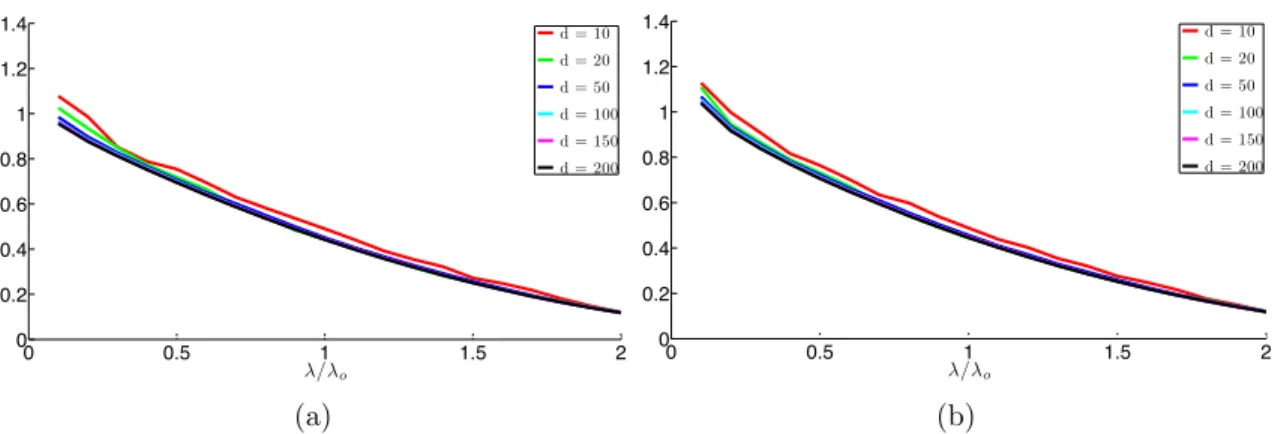
0 0.5 1 1.5 2 0 0.2 0.4 0.6 0.8 1 1.2 1.4 λ/λo d = 10 d = 20 d = 50 d = 100 d = 150 d = 200 (a) 0 0.5 1 1.5 2 0 0.2 0.4 0.6 0.8 1 1.2 1.4 λ/λo d = 10 d = 20 d = 50 d = 100 d = 150 d = 200 (b)
Figure 1: Average number of true discoveries normalized by subspace dimension for values ofλin an interval including the heuristic λo=1/
√
d. (a)σ=0.25. (b)σ=0.5.
correctly in the noiseless setting and does not select columns from other subspaces. Then (2.3) implies thatλhas to scale at least like 1/√d. On the other hand, ˆβ=0 ifλ≥ ∥XTx∥`∞. Now the
informed reader knows that ∥XTx∥`∞ scales at most like √
(logN)/d so that choosing λ around this value yields no discovery (one can refine this argument to show thatλcannot be higher than a constant times 1/√das we would otherwise have a solution that is too sparse). Hence,λis around 1/√d.
It might be possible to compute a precise relationship between λand the expected number of true discoveries in an asymptotic regime in which the number of points and the dimension of the subspace both increase to infinity in a fixed ratio by adapting ideas from [5,6]. We will not do so here as this is beyond the scope of this paper. Rather, we investigate this relationship by means of a numerical study.
Here, we fix a single subspace in Rn with n = 2,000. We use a sampling density equal to
ρ = 5 and vary the dimension d ∈ {10,20,50,100,150,200} of the subspace as well as the noise level σ ∈ {0.25,0.5}. For each data point, we solve (2.2) for different values of λ around the heuristic λo = 1/
√
d, namely, λ ∈ [0.1λo,2λo]. In our experiments, we declare a discovery if an
entry in the optimal solution exceeds 10−3. Figures1a and 1b show the number of discoveries per subspace dimension (the number of discoveries divided by d). One can clearly see that the curves corresponding to various subspace dimensions stack up on top of each other, thereby confirming that a value ofλon the order of 1/√dyields a fixed fraction of true discoveries. Further inspection also reveals that the fraction of true discoveries is around 50% near λ=λo, and around 75% near
λ=λo/2.
2.4.3 The false-true discovery trade off
We now show empirically that in our model choosingλaround 1/√dtypically yields very few false discoveries as well as many true discoveries; this holds with the proviso that the subspaces are of course not very close to each other.
In this simulation, 22 subspaces of varying dimensions in Rn with n = 2,000 have been
in-dependently selected uniformly at random; there are 5, 4, 3, 4, 4, and 2 subspaces of respective dimensions 200, 150, 100, 50, 20 and 10. This is a challenging regime since the sum of the subspace dimensions equals 2,200 and exceeds the ambient dimension (the clean data matrix X has full
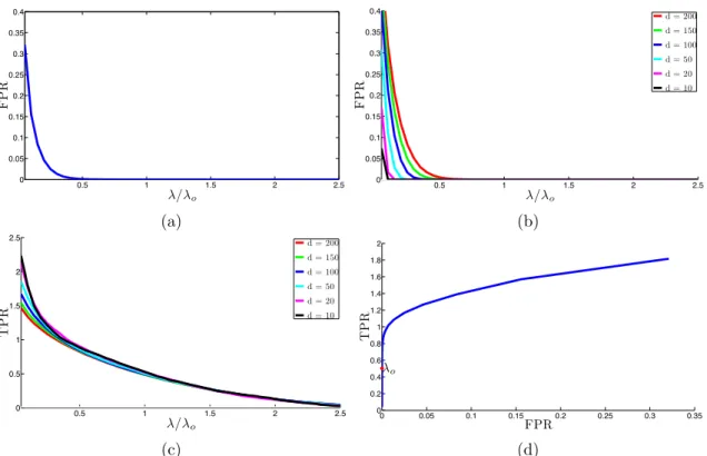
0.5 1 1.5 2 2.5 0 0.05 0.1 0.15 0.2 0.25 0.3 0.35 0.4 λ/λo FP R (a) 0.5 1 1.5 2 2.5 0 0.05 0.1 0.15 0.2 0.25 0.3 0.35 0.4 λ/λo FP R d = 200 d = 150 d = 100 d = 50 d = 20 d = 10 (b) 0.5 1 1.5 2 2.5 0 0.5 1 1.5 2 2.5 λ/λo TPR d = 200 d = 150 d = 100 d = 50 d = 20 d = 10 (c) 0 0.05 0.1 0.15 0.2 0.25 0.3 0.35 0 0.2 0.4 0.6 0.8 1 1.2 1.4 1.6 1.8 2 λo FPR TPR (d)
Figure 2: Performance of LASSO for values ofλin an interval including the heuristic
λo = 1/ √
d. (a) Average number of false discoveries normalized by (n−d) (FPR) on all m sampled data points). (b) FPR for different subspace dimensions. Each curve represents the average FPR over those samples originating from subspaces of the same dimension. (c) Average number of true discoveries per dimension for various dimensions (TPR). (d) TPR vs. FPR (ROC curve). The point corresponding toλ=λo
is marked as a red dot.
rank). We use a sampling density equal toρ=5 for each subspace and set the noise level toσ=0.3. To evaluate the performance of the optimization problem (2.2), we proceed by selecting a subset of columns as follows: for each dimension, we take 100 cases at random belonging to subspaces of that dimension. Hence, the total number of test cases is m=600 so that we only solve m optimization problems (2.2) out of the total N possible cases. Below, β(i) is the solution to (2.2) and β(Si) its restriction to columns with indices in the same subspace. Hence, a nonvanishing entry in β(Si) is a true discovery and, likewise, a nonvanishing entry in βS(ic) is false. For each data point we sweep
the tuning parameter λin (2.2) around the heuristic λo=1/ √
dand work with λ∈ [0.05λo,2.5λo].
In our experiments, a discovery is a value obeying ∣Bij∣ >10−3.
In analogy with the signal detection literature we view the empirical averages of∥β(Sic)∥`0/(n−d)
and ∥β(Si)∥`0/d as False Positive Rate (FPR) and True Positive Rate (TPR). On the one hand,
Figures 2a and 2b show that for values around λ = λo, the FPR is zero (so there are no false
discoveries). On the other hand, Figure 2c shows that the TPR curves corresponding to different dimensions are very close to each other and resemble those in Figure 1 in which all the points belong to the same cluster with no opportunity of making a false discovery. Hence, taking λnear
1/√dgives a performance close to what can be achieved in a noiseless situation. That is to say, we have no false discovery and a number of true discoveries aboutd/2 if we chooseλ=λo. Figure2d
plots TPR versus FPR (a.k.a. the Receiver Operating Characteristic (ROC) curve) and indicates that λ=λo (marked by a red dot) is an attractive trade-off as it provides no false discoveries and
sufficiently many true discoveries.
2.4.4 A two-step procedure
Returning to the selection of the regularization parameter, we would like to use λon the order of 1/√d. However, we do not knowd and proceed by substituting an estimate. In the next section, we will see that we are able to quantify theoretically the performance of the following proposal: (1) run a hard constrained version of the LASSO and use an estimate ˆdof dimension based on the`1 norm of the fitted coefficient sequence; (2) impute a value forλ constructed from ˆd. The two-step procedure is explained in Algorithm2.
Algorithm 2 Two-step procedure with data-driven regularization
for i=1, . . . , N do 1. Solve β⋆=arg min β∈RN ∥β∥`1 subject to ∥yi−Y β∥`2 ≤τ and βi=0. (2.4) 2. Setλ=f(∥β⋆∥`1). 3. Solve ˆ β=arg min β∈RN 1 2∥yi−Y β∥ 2 `2 +λ∥β∥`1 subject to βi=0. 4. SetBi=βˆ. end for
To understand the rationale behind this, imagine we have noiseless data—i. e. Y =X—and are solving (2.1), which simply is our first step (2.4) with the proviso that τ =0. When there are no false discoveries, one can show that the `1 norm of β⋆ is roughly of size
√
d as shown in Lemma
8.2from Section8. This suggests using a multiple of∥β⋆∥`1 as a proxy for
√
d. To drive this point home, take a look at Figure 3a which solves (2.4) with the same data as in the previous example and τ =2σ. The plot reveals that the values of ∥β⋆∥`1 fluctuate around
√
d. This is shown more clearly in Figure3b, which shows that∥β⋆∥`1 is concentrated around
1 4
√
dwith, as expected, higher volatility at lower values of dimension.
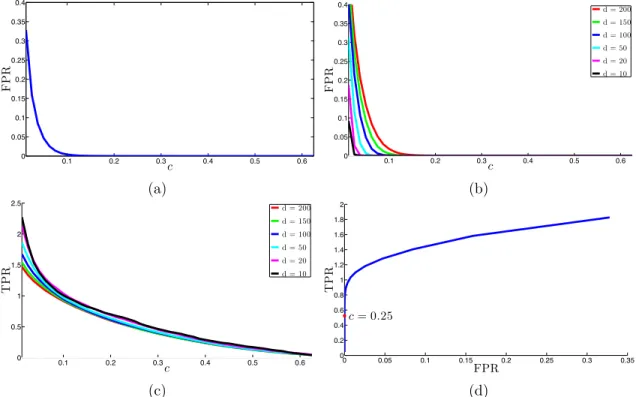
Under suitable assumptions, we shall see in Section 3 that with noisy data, there are simple rules for selecting τ that guarantee, with high probability, that there are no false discoveries. To be concrete, one can take τ = 2σ and f(t) ∝ t−1. Returning to our running example, we have
∥β⋆∥`1 ≈
1 4
√
d. Plugging this into λ= 1/√d suggests taking f(t) ≈ 0.25t−1. The plots in Figure
4 demonstrate that this is indeed effective. Experiments in Section 6 indicate that this is a good choice on real data as well.
The two-step procedure requires solving two LASSO problems for each data point and is useful when there are subspaces of large dimensions (in the hundreds, say) and some others of low-dimensions (three or four, say). In some applications such as motion segmentation in computer
0 100 200 300 400 500 600 0.5 1 1.5 2 2.5 3 3.5 4 (a) 0 100 200 300 400 500 600 0.2 0.25 0.3 0.35 0.4 (b)
Figure 3: Optimal values of (2.4) for 600 samples using τ =2σ. The first 100 values correspond to points originating from subspaces of dimension d= 200, the next 100 from those of dimension d=150, and so on through d∈ {100,50,20,10}. (a) Value of
∥β∗∥` 1. (b) Value of∥β ∗∥ `1/ √ d.
vision, the dimensions of the subspaces are all equal and known in advance. In this case, one can forgo the two-step procedure and simply set λ=1/√d.
3
Theoretical Results
This section presents our main theoretical results concerning the performance of the two-step pro-cedure (Algorithm 2). We make two assumptions:
• Affinity condition. We say that a subspace S` obeys the affinity condition if
max
k∶k≠` aff(S`, Sk) ≤κ0/logN , (3.1)
whereκ0 a fixed numerical constant.
• Sampling condition. We say that subspaceS` obeys thesampling condition if
ρ`≥ρ⋆, (3.2)
whereρ⋆ is a fixed numerical constant.
The careful reader might argue that we should require lower affinity values as the noise level increases. The reason why σ does not appear in (3.1) is that we assumed a bounded noise level. For higher values ofσ, the affinity condition would read as in (3.1) with a right-hand side equal to
κ= κ0 logN −σ √ d` 2nlogN. 3.1 Main results
From here on we use d(i) to refer to the dimension of the subspace the vector yi originates from.
0.1 0.2 0.3 0.4 0.5 0.6 0 0.05 0.1 0.15 0.2 0.25 0.3 0.35 0.4 c FP R (a) 0.1 0.2 0.3 0.4 0.5 0.6 0 0.05 0.1 0.15 0.2 0.25 0.3 0.35 0.4 c FP R d = 200 d = 150 d = 100 d = 50 d = 20 d = 10 (b) 0.1 0.2 0.3 0.4 0.5 0.6 0 0.5 1 1.5 2 2.5 c TPR d = 200 d = 150 d = 100 d = 50 d = 20 d = 10 (c) 0 0.05 0.1 0.15 0.2 0.25 0.3 0.35 0 0.2 0.4 0.6 0.8 1 1.2 1.4 1.6 1.8 2 c= 0.25 FPR TPR (d)
Figure 4: Performance of the two-step procedure using τ = 2σ and f(t) = ct−1 for values of c around the heuristic c=0.25. (a) False positive rate (FPR). (b) FPR for various subspace dimensions. (c) True positive rate (TPR). (d) TPR vs. FPR.
Theorem 3.1 (No false discoveries) Assume that the subspace attached to theith column obeys the affinity and sampling conditions and that the noise level σ is bounded as in (1.2), whereσ⋆ is a sufficiently small numerical constant. In Algorithm 2, take τ = 2σ and f(t) obeying f(t) ≥
0.707σt−1. Then with high probability,4 there is no false discovery in theith column of B.
Theorem 3.2 (Many true discoveries) Consider the same setup as in Theorem3.1withf also obeying f(t) ≤ct−1 for some numerical constant c. Then with high probability,5 there are at least
c0
d(i)
log2(ρ(i))
true discoveries in the ith column (c0 is a positive numerical constant).
The above results indicate that the algorithm works correctly in fairly broad conditions. To give an example, assume two subspaces of dimensiondoverlap in a smaller subspace of dimensionsbut are orthogonal to each other in the remaining directions (equivalently, the first s principal angles are 0 and the rest are π/2). In this case, the affinity between the two subspaces is equal to √s/d
and (3.1) allowssto grow almost linearly in the dimension of the subspaces. Hence, subspaces can have intersections of large dimensions. In contrast, previous work with perfectly noiseless data [18] would impose to have a first principal angle obeying ∣cosθ(1)∣ ≤ 1/√d so that the subspaces are practically orthogonal to each other. Whereas our result shows that we can have an average of the cosines practically constant, the condition in [18] asks that the maximum cosine be very small.
In the noiseless case, [41] showed that when the sampling condition holds and max
k∶k≠` aff(S`, Sk) ≤κ0 √
logρ`
logN ,
(albeit with slightly different values κ0 and ρ⋆), then applying the noiseless version (2.1) of the algorithm also yields no false discoveries. Hence, with the proviso that the noise level is not too large, conditions under which the algorithm is provably correct are essentially the same.
Earlier, we argued that we would like to have, if possible, an algorithm provably working at (1) high values of the affinity parameters and (2) low values of the sampling density as these are the conditions under which the clustering problem is challenging. (Another property on the wish list is the ability to operate properly with high noise or low SNR and this is discussed next.) In this context, since the affinity is at most one, our results state that the affinity can be within a log factor from this maximum possible value. The number of samples needed per subspace is minimal as well. That is, as long as the density of points on each subspace is larger than a constant ρ>ρ⋆, the algorithm succeeds.
We would like to have a procedure capable of making no false discoveries and many true discov-eries at the same time. Now in the noiseless case, whenever there are no false discovdiscov-eries, the ith column contains exactlyd(i)true discoveries. Theorem3.2states that as long as the noise levelσis less than a fixed numerical constant, the number of true discoveries is roughly on the same order as in the noiseless case. In other words, a noise level of this magnitude does not fundamentally affect
4probability at least 1−2e−γ1n−6e−γ2d(i)−e− √
N(i)d(i)−N(i)−(2d(i)−1)−12
N, for fixed numerical constantsγ1,γ2.
5probability at least 1−2e−γ1n−6e−γ2d(i)−e− √
N(i)d(i)−N(i)−(2d(i)−1)−10
N −
4
N(i), for fixed numerical constantsγ1,
ï2 ï1 0 1 2 0 500 1000 1500 (a) ï2 ï1 0 1 2 0 20 40 60 80 100 (b)
Figure 5: Histograms of the true discovery values from the two step procedure with
c=0.25 (multiplied by√d). (a)d=200. (b) d=20.
the performance of the algorithm. This holds even when there is great variation in the dimensions of the subspaces, and is possible because λis appropriately tuned in an adaptive fashion.
The number of true discoveries is shown to scale at least like dimension over the squared log of the density (we conjecture that it should just be the log of the density). This may suggest that the number of true discoveries decreases (albeit very slowly) as the sampling density increases. This behavior is to be expected: when the sampling density becomes exponentially large (in terms of the dimension of the subspace) the number of true discoveries become small since we need fewer columns to synthesize a point.
Theorem 3.2 establishes that there are many true discoveries. This would not be useful for clustering purposes if there were only a handful of very large true discoveries and all the others of negligible magnitude. The reason is that the similarity matrix W would then be close to a sparse matrix and we would run the risk of splitting true clusters. This is not what happens and our proofs can show this although we do not do this in this paper for lack of space. Rather, we demonstrate this property empirically. On our running example, Figures5aand5b show that the histograms of appropriately normalized true discovery values resemble a bell-shaped curve.
Finally, we would like to comment on the fact that our main results hold when λ belongs to a fairly broad range of values. First, when all the subspaces have small dimensions, one can choose the same value ofλfor all the data points since 1/√dis essentially constant. Hence, when we know a priori that we are in such a situation, there may be no need for the two step procedure. (We would still recommend the conservative two-step procedure because of its superior empirical performance on real data.) Second, the proofs also reveal that if we have knowledge of the dimension of the largest subspace dmax, the first theorem holds with a fixed value of λ proportional to σ/
√
dmax. Third, when the subspaces themselves are drawn at random, the first theorem holds with a fixed value of λ proportional to σ(logN)/√n. (Both these statements follow by plugging these values of λ in the proofs of Section 8 and we omit the calclulations.) We merely mention these variants to give a sense of what our theorems can also give. As explained earlier, we recommend the more conservative two-step procedure with the proxy for 1/√d. The reason is that using a higher value of
λallows for a larger value ofκ0, which says that the subspaces can be even closer. In other words, we can function in a more challenging regime. To drive this point home, consider the noiseless problem. When the subspaces are close, the equality constrained `1 problem may yield some false discoveries. However, if we use the LASSO version—even though the data is noiseless—we may
end up with no false discoveries while maintaining sufficiently many true discoveries.
4
The Bias-corrected Dantzig Selector
One can think of other ways of performing the first step in Algorithm 1and this section discusses another approach based on a modification of the Dantzig selector, a popular sparse regression technique [15]. Unlike the two-step procedure, we do not claim any theoretical guarantees for this method and shall only explore its properties on real and simulated data.
Applied directly to our problem, the Dantzig selector takes the form min
β∈RN ∥β∥`1 subject to ∥Y
T
(−i)(yi−Y β)∥`∞≤λ and βi=0, (4.1)
where Y(−i) is Y with the ith column deleted. However, this is hardly suitable since the design
matrixY is corrupted. Interestingly, recent work [38,39] has studied the problem of estimating a sparse vector from the standard linear model under uncertainty in the design matrix. The setup in these papers is close to our problem and we propose a modified Dantzig selection procedure inspired but not identical to the methods set forth in [38,39].
4.1 The correction
If we had clean data, we would solve (2.1); this is (4.1) withY =X andλ=0. LetβIbe the solution to this ideal noiseless problem. Applied to our problem, the main idea in [38,39] would be to find a formulation that resembles (4.1) with the property that βI is feasible. Since xi = X(−i)βI(−i),
observe that we have the following decomposition:
Y(−Ti)(yi−Y βI) = (X(−i)+Z(−i))T(zi−ZβI)
=X(−Ti)(zi−ZβI) +Z(−Ti)zi−Z(−Ti)Zβ I.
Then the conditional mean is given by
E[Y(−Ti)(yi−Y βI) ∣X] = −EZ(−Ti)Z(−i)βI(−i)= −σ2βI(−i).
In other words,
σ2βI(−i)+Y(−Ti)(yi−Y βI) =ξ
whereξ has mean zero. In Section4.2, we compute the variance of thejth componentξj, given by
Eξj2= σ 2 n(1+ ∥β I∥2 `2) + σ4 n(1+ (β I j)2+ ∥βI∥2`2). (4.2)
Owing to our Gaussian assumptions,∣ξj∣shall be smaller than 3 or 4 times this standard deviation,
say, with high probability.
Hence, we may want to consider a procedure of the form min β∈RN ∥β∥`1 subject to ∥Y T (−i)(yi−Y β) +σ 2β (−i)∥`∞≤λ and βi=0. (4.3)
It follows that if we take λto be a reasonable multiple of (4.2), thenβI would obey the constraint in (4.3) with high probability. Hence, we would need to approximate the variance (4.2). Numerical
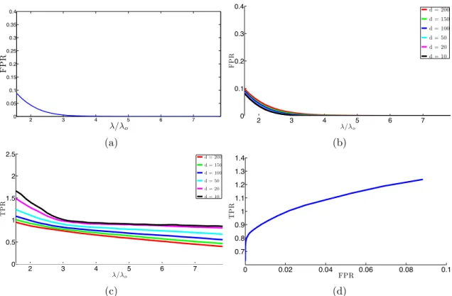
2 3 4 5 6 7 0 0.05 0.1 0.15 0.2 0.25 0.3 0.35 0.4 λ/λo FP R (a) 2 3 4 5 6 7 0 0.1 0.2 0.3 0.4 λ/λo FPR d = 200 d = 150 d = 100 d = 50 d = 20 d = 10 (b) 2 3 4 5 6 7 0 0.5 1 1.5 2 2.5 λ/λo TP R d = 200 d = 150 d = 100 d = 50 d = 20 d = 10 (c) 0 0.02 0.04 0.06 0.08 0.1 0.7 0.8 0.9 1 1.1 1.2 1.3 1.4 FPR TP R (d)
Figure 6: Performance of the bias-corrected Dantzig selector for values of λthat are multiples of the heuristicλo=
√
2/n σ√1+σ2. (a) False positive rate (FPR). (b) FPR for different subspace dimensions. (c) True positive rate (TPR). (d) TPR vs. FPR.
simulations together with asymptotic calculations presented in Appendix C give that ∥βI∥`2 ≤ 1
with very high probability. Thus neglecting the term in(βI j)2, Eξ2j ≈σ 2 n(1+σ 2)( 1+ ∥βI∥2`2) ≤2σ 2 n(1+σ 2) .
This suggests takingλto be a multiple of√2/n σ√1+σ2. This is interesting because the parameter
λdoes not depend on the dimension of the underlying subspace. We shall refer to (4.3) as the bias-corrected Dantzig selector, which resembles the proposal in [38,39] for which the constraint is a bit more complicated and of the form∥Y(−Ti)(yi−Y β) +D(−i)β∥`∞≤µ∥β∥`1+λ.
To get a sense about the validity of this proposal, we test it on our running example by varying
λ ∈ [λo,8λo] around the heuristic λo = √
2/n σ√1+σ2. Figure 6 shows that good results are achieved around factors in the range [4,6].
In our synthetic simulations, both the two-step procedure and the corrected Dantzig selector seem to be working well in the sense that they yield many true discoveries while making very few false discoveries, if any. Comparing Figures 6b and 6c with those from Section 2 show that the corrected Dantzig selector has more true discoveries for subspaces of small dimensions (they are essentially the same for subspaces of large dimensions); that is, the two-step procedure is more conservative when it comes to subspaces of smaller dimensions. As explained earlier this is due to our conservative choice ofλresulting in a TPR about half of what is obtained in a noiseless setting. Having said this, it is important to keep in mind that in these simulations the planes are drawn
at random and as a result, they are sort of far from each other. This is why a less conservative procedure can still achieve a low FPR. When smaller subspaces are closer to each other or when the statistical model does not hold exactly as in real data scenarios, a conservative procedure may be more effective. In fact, experiments on real data in Section6confirm this and show that for the corrected Dantzig selector, one needs to choose values much larger thanλo to yield good results.
4.2 Variance calculation
By definition,
ξj = ⟨xj,zi−ZβI⟩ + ⟨zj,zi⟩ − (zjTzj−σ2)βjI− ∑ k∶k≠i,j
zjTzkβkI∶=I1+I2+I3+I4.
A simple calculation shows that for`1≠`2, Cov(I`1, I`2) =0 so that Eξj2= 4 ∑ `=1 Var(I`). We compute Var(I1) = σ2 n (1+ ∥β I∥2 `2), Var(I2) = σ4 n , Var(I3) = σ4 n 2(β I j)2, Var(I4) = σ4 n [∥β I∥2 `2− (β I j)2] and (4.2) follows.
5
Comparisons With Other Works
We now briefly comment on other approaches to subspace clustering. Since this paper is theoretical in nature, we shall focus on comparing theoretical properties and refer to [19], [47] for a detailed comparison about empirical performance. Three themes will help in organizing our discussion.
• Tractability. Is the proposed method or algorithm computationally tractable? • Robustness. Is the algorithm provably robust to noise and other imperfections?
• Efficiency. Is the algorithm correctly operating near the limits we have identified above? In our model, how many points do we need per subspace? How large can the affinity between subspaces be?
One can broadly classify existing subspace clustering techniques into three categories, namely, algebraic, iterative and statistical methods.
Methods inspired from algebraic geometry have been introduced for clustering purposes. In this area, a mathematically intriguing approach is thegeneralized principal component analysis(GPCA) presented in [48]. Unfortunately, this algorithm is not tractable in the dimension of the subspaces, meaning that a polynomial-time algorithm does not exist. Another feature is that GPCA is not robust to noise although some heuristics have been developed to address this issue, see e.g. [32]. As far as the dependence upon key parameters is concerned, GPCA is essentially optimal. An interesting approach to make GPCA robust is based on semidefinite programming [36]. However,
this novel formulation is still intractable in the dimension of the subspaces and it is not clear how the performance of the algorithm depends upon the parameters of interest.
A representative example of an iterative method—the term is taken from the tutorial [47]—is the K-subspace algorithm [43], a procedure which can be viewed as a generalization of K-means. Here, the subspace clustering problem is formulated as a non-convex optimization problem over the choice of bases for each subspace as well as a set of variables indicating the correct segmentation. A cost function is then iteratively optimized over the basis and the segmentation variables. Each iteration is computationally tractable. However, due to the non-convex nature of the problem, the convergence of the sequence of iterates is only guaranteed to a local minimum. As a consequence, the dependence upon the key parameters is not well understood. Furthermore, the algorithm can be sensitive to noise and outliers. Other examples of iterative methods may be found in [1,9,29,52]. Statistical methods typically model the subspace clustering problem as a mixture of degenerate Gaussian observations. Two such approaches are mixtures of probabilistic PCA (MPPCA) [42] andagglomerative lossy compression(ALC) [30]. MPPCA seeks to compute a maximum-likelihood estimate of the parameters of the mixture model by using an expected-maximization (EM) style algorithm. ALC searches for a segmentation of the data by minimizing the code length necessary (with a code based on Gaussian mixtures) to fit the points up to a given distortion. Once more, due to the non-convex nature of these formulations, the dependence upon the key parameters and the noise level is not understood.
Many other methods apply spectral clustering to a specially constructed graph [2,8,16,23,50,53]. They share the same difficulties as stated above and [47] discusses advantages and drawbacks. An approach similar to SSC is called low-rank representation (LRR) [27]. The LRR algorithm is tractable but its robustness to noise and its dependence upon key parameters is not understood. The work in [26] formulates the robust subspace clustering problem as a non-convex geometric minimization problem over the Grassmanian. Because of the non-convexity, this formulation may not be tractable. On the positive side, this algorithm is provably robust and can accommodate noise levels up to O(1/(Ld3/2)). However, the densityρ required for favorable properties to hold is an unknown function of the dimensions of the subspaces (e.g. ρ could depend on d in a super polynomial fashion). Also, the bound on the noise level seems to decrease as the dimension d
and number of subspaces L increases. In contrast, our theory requires ρ ≥ ρ⋆ where ρ⋆ is a fixed numerical constant. While this manuscript was under preparation we learned of [20] which establishes robustness to sparse outliers but with a dependence on the key parameters that is super-polynomial in the dimension of the subspaces demanding ρ ≥ C0dlogn. (Numerical simulations in [20] seem to indicate thatρ cannot be a constant.)
Finally, the papers [28,38,39] also address regression under corrupted covariates. However, there are three key differences between these studies and our work. First, our results show that LASSO without any change is robust to corrupted covariates whereas these works require modifications to either LASSO or the Dantzig selector. Second, the modeling assumptions for the uncorrupted covariates are significantly different. These papers assume that X has i.i.d. rows and obeys the
restricted eigenvalue condition (REC) whereas we have columns sampled from a mixture model so that the design matrices do not have much in common. Last, for clustering and classification purposes, we need to verify that the support of the solution is correct whereas these works establish closeness to an oracle solution in an`2 sense. In short, our work is far closer to multiple hypothesis testing.
6
Numerical Experiments
In this section, we perform numerical experiments corroborating our main results and suggesting their applications to temporal segmentation of motion capture data. In this application we are given sensor measurements at multiple joints of the human body captured at different time instants. The goal is to segment the sensory data so that each cluster corresponds to the same activity. Here, each data point corresponds to a vector whose elements are the sensor measurements of different joints at a fixed time instant.
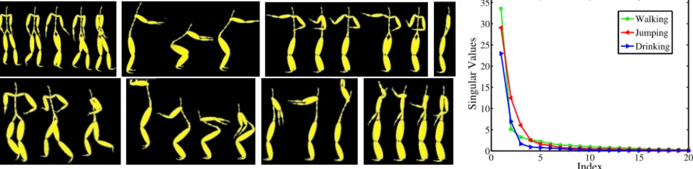
We use the Carnegie Mellon Motion Capture dataset (available at http://mocap.cs.cmu.edu), which contains 149 subjects performing several activities (data are provided in [54]). The motion capture system uses 42 markers per subject. We consider the data from subject 86 in the dataset, consisting of 15 different trials, where each trial comprises multiple activities. We use trials 2 and 5, which feature more activities (8 activities for trial 2 and 7 activities for trial 5) and are, therefore, harder examples relative to the other trials. Figure 7 shows a few snapshots of each activity (walking, squatting, punching, standing, running, jumping, arms-up, and drinking) from trial 2. The right plot in Figure 7 shows the singular values of three of the activities in this trial. Notice that all the curves have a low-dimensional knee, showing that the data from each activity lie in a low-dimensional subspace of the ambient space (n=42 for all the motion capture data).
0 5 10 15 20 0 5 10 15 20 25 30 35 Index Singular Values Walking Jumping Drinking
Figure 7: Left: eight activities performed by subject 86 in the CMU motion cap-ture dataset: walking, squatting, punching, standing, running, jumping, arms-up, and drinking. Right: singular values of the data from three activities (walking, jumping, drinking) show that the data from each activity lie approximately in a low-dimensional subspace.
We compare three different algorithms: a baseline algorithm, the two-step procedure and the bias-corrected Dantzig selector. We evaluate these algorithms based on theclustering error. That is, we assume knowledge of the number of subspaces and apply spectral clustering to the similarity matrix built by the algorithm. After the spectral clustering step, the clustering error is simply the ratio of misclassified points to the total number of points. We report our results on half of the examples—downsampling the video by a factor 2 keeping every other frame—as to make the problem more challenging. (As a side note, it is always desirable to have methods that work well on a smaller number of examples as one can use split-sample strategies for tuning purposes).6
As a baseline for comparison, we apply spectral clustering to a standard similarity graph built
6We have adopted this subsampling strategy to make our experiments reproducible. For tuning purposes, a random strategy may be preferrable.
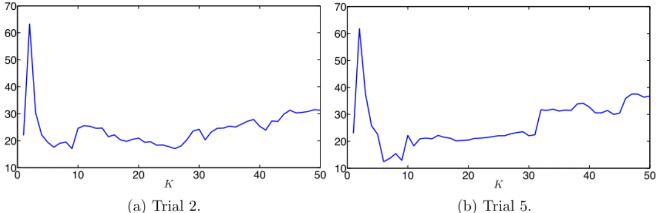
0 10 20 30 40 50 10 20 30 40 50 60 70 K (a) Trial 2. 0 10 20 30 40 50 10 20 30 40 50 60 70 K (b) Trial 5.
Figure 8: Minimum clustering error (%) for each K in the baseline algorithm.
by connecting each data point to its K-nearest neighbors. For pairs of data points, yi and yj,
that are connected in the K-nearest neighbor graph, we define the similarities between them by
Wij =exp(−∥yi−yj∥22/t), wheret>0 is a tuning parameter (a.k.a. temperature). For pairs of data points, yi and yj, that are not connected in theK-nearest neighbor graph, we set Wij =0. Thus,
pairs of neighboring data points that have small Euclidean distances from each other are considered to be more similar, since they have high similarity Wij. We then apply spectral clustering to the
similarity graph and measure the clustering error. For each value of K, we record the minimum clustering error over different choices of the temperature parameter t >0 as shown in Figures 8a
and 8b. The minimum clustering error for trials 2 and 5 are 17.06% and 12.47%.
For solving the LASSO problems in the two-step procedure, we developed a computational routine made publicly available [44] based on TFOCS [7] solving the optimization problems in parallel. For the corrected Dantzig selector we use a homotopy solver in the spirit of [45].
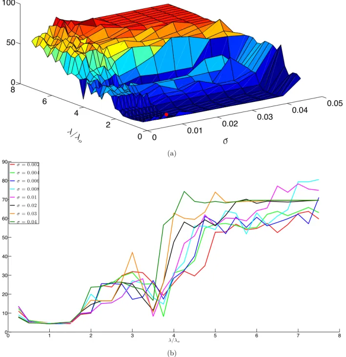
For both the two-step procedure and the bias-corrected Dantzig selector we normalize the data points as a preprocessing step. We work with a noise σ in the interval [0.001,0.045], and for each value of σ, we vary λ around 1/λo = 4∥β⋆∥`1 and λo =
√
2/n σ√1+σ2. After building the similarity graph from the sparse regression output, we apply spectral clustering as explained earlier. Figures9a,9band 10show the clustering error (on trial 5) and the red point indicates the location where the minimum clustering error is reached. Figures 9a and 9b show that for the two-step procedure the value of the clustering error is not overly sensitive to the choice of σ—especially around λ = λo. Notice that the clustering error for the robust versions of SSC are significantly
lower than the baseline algorithm for a wide range of parameter values. The reason the baseline algorithm performs poorly in this case is that there are many points that are in small Euclidean distances from each other, but belong to different subspaces.
Finally a summary of the clustering errors of these algorithms on the two trials are reported in Table 1. Robust versions of SSC outperform the baseline algorithm. This shows that the multiple subspace model is better for clustering purposes. The two-step procedure seems to work slightly better than the corrected Dantzig selector for these two examples. Table 2 reports the optimal parameters that achieve the minimum clustering error for each algorithm. The table indicates that on real data, choosingλclose toλoalso works very well. Also, one can see that in comparison with
the synthetic simulations of Section4, a more conservative choice of the regularization parameterλ
is needed for the corrected Dantzig selector asλneeds to be chosen much higher thanλoto achieve
0 0.01 0.02 0.03 0.04 0.05 0 2 4 6 80 50 100
σ
λ/λ o (a) 0 1 2 3 4 5 6 7 8 0 10 20 30 40 50 60 70 80 90 λ/λo σ= 0.002 σ= 0.004 σ= 0.006 σ= 0.008 σ= 0.01 σ= 0.02 σ= 0.03 σ= 0.04 (b)Figure 9: Clustering error (%) for different values of λand σ on trial 5 using the two step procedure (a) 3D plot (minimum clustering error appears in red). (b) 2D cross sections.
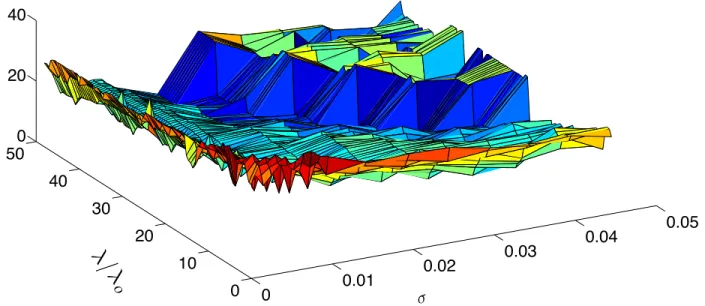
0 0.01 0.02 0.03 0.04 0.05 0 10 20 30 40 500 20 40 σ
λ/
λ
oFigure 10: Clustering error (%) for different values of λ and σ on trial 5 using the corrected Dantzig Selector.
0.65 0.7 0.75 0.8 0.85 0.9 0.95 trial 2 trial 5
Figure 11: Box plot of the affinities between subspaces for trials 2 and 5.
close to each other and are not drawn at random as was the case with our synthetic data. To get a sense of the affinity values, we fit a subspace of dimensiond` to theN` data points from the `th
group, where d` is chosen as the smallest nonnegative integer such that the partial sum of the d`
top singular values is at least 90% of the total sum. Figure 11 shows that the affinities are higher than 0.75 for both trials.
7
Discussion and Open Problems
In this paper, we have developed a tractable algorithm that can provably cluster data points in a fairly challenging regime in which subspaces can overlap along many dimensions and in which the number of points per subspace is rather limited. Our results about the performance of the robust SSC algorithm are expressed in terms of interpretable parameters. This is not a trivial achievement: one of the challenges of the theory for subspace clustering is precisely that performance depends on many different aspects of the problem such as the dimension of the ambient space, the number
Baseline Algorithm Two-step procedure Corrected Dantzig selector
Trial 2 17.06% 3.54% 9.53%
Trial 5 12.47% 4.35% 4.92%
Table 1: Minimum clustering error.
Baseline algorithm Two-step procedure Corrected Dantzig selector Trial 2 K=9, t=0.0769 σ=0.03 , λ=1.25λo σ=0.004 ,λ=41.5λo
Trial 5 K=6, t=0.0455 σ=0.01,λ=λo σ=0.03 , λ=45.5λo
Table 2: Optimal parameters.
of subspaces, their dimensions, their relative orientations, the distribution of points around each subspace, the noise level, and so on. Nevertheless, these results only offer a starting point as our work leaves open lots of questions, and at the same time, suggests topics for future research. Before presenting the proofs, we would like to close by listing a few questions colleagues may find of interest.
• We have shown that while having the affinities and sampling densities near what is information theoretically possible, robust versions of SSC that can accommodate noise levels σ of order one exist. It would be interesting to establish fundamental limits relating the key parameters to the maximum allowable noise level. What is the maximum allowable noise level for any algorithm regardless of tractability?
• It would be interesting to extend the results of this paper to a deterministic model where both the orientation of the subspaces and the noiseless samples are non-random. We leave this to a future publication.
• Our work in this paper concerns the construction of the similarity matrix and the correctness of sparse regression techniques. The full algorithm then applies clustering techniques to clean up errors introduced in the first step. It would be interesting to develop theoretical guarantees for this step as well. A potential approach is the interesting formulation developed in [4]. • A natural direction is the development of clustering techniques that can provably operate with
missing and/or sparsely corrupted entries (the work [41] only deals with grossly corrupted columns). The work in [20] provides one possible approach but requires a very high sampling density as we already mentioned. The paper [19] develops another heuristic approach without any theoretical justification.
• One of the advantages of the suggested scheme is that it is highly parallelizable. When the al-gorithm is run sequentially, it would be interesting to see whether one can reuse computations to solve all the`1-minimization problems more effectively.
8
Proofs
We prove all of our results in this section. Before we begin, we introduce some notation. If A is a matrix with N columns andT a subset of {1, . . . , N}, AT is the submatrix with columns in T.
Similarly, xT is the restriction of the vector x to indices inT. Throughout we use Lm to denote
logm up to a fixed numerical constant. The value of this constant may change from line to line. Likewise,C is a generic numerical constant whose value may change at each occurrence.
Next, we work with y∶=y1 for convenience, assumed to originate from S1, which is no loss of generality. It is also convenient to partition Y as {Y(1),Y(2), . . . ,Y(L)}, where for each `, Y(`)
are those noisy columns from subspaceS`; when`=1, we exclude the responsey1 fromY(1). With this notation, the problem (2.2) takes the form
min β∈RN−1 1 2∥y− (Y (1)β(1)+. . .+Y(L)β(L))∥2 `2+ λ∥β(1)∥ `1 + . . .+λ∥β(L)∥ `1 . (8.1)
Throughout, y∥/Y∥(1) denotes the projection of the vector/matrix y/Y(1) onto S1. Similarly, we use y⊥ to denote projection onto the orthogonal complement S1⊥; hence, y =y∥+y⊥ and Y(1) = Y∥(1)+Y⊥(1). Moreover,U1∈Rn×d andU1⊥∈Rn×(n−d) are orthonormal bases forS1 and S1⊥.
Since y∥ = x+z∥ with ∥x∥`2 = 1 and E∥z∥∥
2
`2 = σ
2d/n, it is obvious that under the stated assumptions, ∥y∥∥`2 ∈ [3/4,5/4] with very high probability as shown in Lemma A.4. The same
applies to all the columns of Y∥(1). From now on, we will operate under these two assumptions, which hold simultaneously over an event of probability at least 1−1/N2d1−1
1 .
8.1 Intermediate results
In this section, we record a few important results that shall be used to establish the no-false and many true discoveries theorems. Now the reader interested in our proofs may first want to pass over this section rather quickly, and return to it once it is clear how our arguments reduce to the technical lemmas below.
8.1.1 Preliminaries
Our first lemma rephrases Lemma 7.5 in [41] and bounds the size of the dot product between random vectors. We omit the proof.
Lemma 8.1 Let A∈Rd1×N1 be a matrix with columns sampled uniformly at random from the unit
sphere of Rd1, w∈Rd2 be a vector sampled uniformly at random from the unit sphere of Rd2 and
independent of A and Σ∈Rd1×d2 be a deterministic matrix. We have
∥ATΣw∥`∞ ≤√logalogb√∥Σ∥F d1√d2
, (8.2)
with probability at least 1−√2
a−
2√N1
b .
We are interested in this because (8.2) relates the size of the dot products with the affinity between subspaces as follows: suppose the unit-norm vector xi is drawn uniformally at random from Si,
then
X(j)Txi =ATΣw;
A and w are as in the lemma andΣ=U(j)TU(i), where U(j) (resp. U(i)) is an orthobasis forSj
(resp. Si). By definition,∥Σ∥F = √
8.1.2 The first step of Algorithm 2
As claimed in Section2, the first step of Algorithm2 returns an optimal value that is a reasonable proxy for the unknown dimension.
Lemma 8.2 Let Val(Step 1)be the optimal value of (2.4) withτ =2σ. Assume ρ1>ρ⋆ as earlier.
Then 1 10 √ d1 logρ1 ≤ Val(Step 1)≤2√d1. (8.3)
The upper bound holds with probability at least 1−eγ1n−e−γ2d1. The lower bound holds with
probability at least 1−e−γ3d1−10
N.
Proof We begin with the upper bound. Letβ0=X(1)
T
(X(1)X(1)T)−1xbe the minimum`2-norm solution to the noiseless problem Xβ0=x. We show thatβ0 is feasible for (2.4). We have
y−Y β0 =x−Xβ0+ (z−Zβ0) =z−Zβ0, which gives
L(z−Zβ0∣X,x) = N (0, VIn), V = (1+ ∥β0∥2`2)σ2/n
(the notation L(Y∣X) is the conditional law ofY given X). Hence, the conditional distribution of
∥z−Zβ0∥2`2 is that of a chi square and (A.1) gives
∥z−Zβ0∥`2 ≤
√
2(1+ ∥β0∥2`2)σ
with probability at least 1−e−γ1n. On the other hand,
∥β0∥`2 ≤ ∥
x∥`2
σmin(X(1)) and applying LemmaA.2gives
∥β0∥`2 ≤ 1 √N 1 d1 −2 ,
which holds with probability at least 1−e−γ2d1. IfN
1>9d1, then ∥β0∥`2 ≤1 and thusβ0 is feasible.
Therefore, ∥β⋆∥`1 ≤ ∥β0∥`1 ≤ √ N1∥β0∥`2 ≤ √ d1 1−2√d1 N1 ≤2√d1, where the last inequality holds provided thatN1≥16d1.
We now turn to the lower bound and letβ⋆ be an optimal solution. Notice that∥y∥−Y∣∣β⋆∥`2 ≤
∥y−Y β⋆∥`2 ≤2σ so that β⋆ is feasible for
min ∥β∥`1 subject to ∥y∥−Y∥β∥`
2 ≤2σ. (8.4)
We bound the optimal value of this program from below. The dual of (8.4) is max ⟨y∥,ν⟩ −2σ∥ν∥`
2 subject to ∥Y
T
Slater’s condition holds and the primal and dual optimal values are equal. To simplify notation set
A=Y∥(1). Define
ν⋆∈arg max ⟨y∥,ν⟩ subject to ∥ATν∥`∞ ≤1.
Notice that ν⋆ has random direction on subspace S1. Therefore, combining Lemmas 8.1, A.1, and B.4 together with the affinity condition implies that for ` ≠ 1, ∥Y∣∣(`)Tν∗∥`∞ ≤ 1 with high
probability. In short, ν⋆ is feasible for (8.5).
Since y∥has random direction, the arguments (with t=1/6) in Step 2 of the proof of Theorem 2.9 in [41] give ⟨y∥,ν⋆⟩ ≥ √1 2πe √ d1 logρ1 . Also, by Lemma B.4, ∥ν⋆∥` 2 ≤ 16 3 √ d1 logρ1 .
Since ν⋆ is feasible for (8.5), the optimal value of (8.5) is greater or equal than
⟨y∥,ν⋆⟩ −2σ∥ν⋆∥`2 ≥ 1 10 √ d1 logρ1 ,
where the inequality follows from the bound on the noise level. This concludes the proof.
8.1.3 The reduced and projected problems
When there are no false discoveries, the solution to (8.1) coincides with that of thereduced problem
ˆ β(1)∈arg min1 2∥y−Y (1)β(1)∥2 `2+ λ∥β(1)∥ `1 . (8.6)
Not surprisingly, we need to analyze the properties of the solution to this problem. In particular, we would like to understand something about the orientation and the size of the residual vector
y−Y(1)βˆ(1).
A problem close to (8.6) is the projected problem
˜ β(1)∈arg min1 2∥y∥−Y (1) ∥ β(1)∥ 2 `2+ λ∥β(1)∥ `1 . (8.7)
The difference with the reduced problem is that the goodness of fit only involves the residual sum of squares of the projected residuals. Intuitively, the solutions to the two problems (8.6) and (8.7) should be close. Our strategy is to gain some insights about the solution to the reduced problem by studying the properties of the projected problem.
8.1.4 Properties of the projected problem
Lemma 8.3 Let β˜(1) be any solution to the projected problem and assume that N1/d1 ≥ ρ⋆ as
before. Then there exists an absolute constant C such that for all λ>0,
∥β˜(1)∥
`2 ≤
C (8.8)
holds with probability at least 1−5e−γ1d1−e−
√
N1d1.
This estimate shall play a crucial role in our arguments. It is a consequence of sharp estimates obtained by Wojtaszczyk [49] in the area of compressed sensing. As not to interrupt the flow, we postpone its proof to Section8.3.
In the asymptotic regime (ρ1 = N1/d1 fixed and d1 → ∞), one can sharpen the upper bound (8.8) by taking C=1. This leverages the asymptotic theory developed in [5] and [6] as explained in AppendixC.
8.1.5 Properties of the reduced problem
We now collect two important facts about the residuals to the reduced problem. The first concerns their orientation.
Lemma 8.4 (Isotropy of the residuals) The projection of the residual vector r=y−Y(1)βˆ(1)
onto either S1 or S1⊥ has uniform orientation.
Proof Consider any unitary transformationU∥ (resp.U⊥) leaving S1 (resp. S1⊥) invariant. Since 1 2∥U ∥(y ∥−Y∥(1)β(1))∥ 2 `2 + 1 2∥U ⊥(y ⊥−Y⊥(1)β(1))∥ 2 `2 + λ∥β(1)∥ `1 = 21∥y∥−Y∥(1)β(1)∥2 `2+ 1 2∥y⊥−Y (1) ⊥ β(1)∥ 2 `2+ λ∥β(1)∥ `1 ,
the LASSO functional is invariant and this gives ˆ
β(1)(U∥y∥,U⊥y⊥,U∥Y∥(1),U⊥Y⊥(1)) =βˆ(1)(y∥,y⊥,Y∥(1),Y⊥(1)).
Letr∥(y∥,Y∥(1)) =y∥−Y∥(1)βˆ(1)andr⊥(y⊥,Y⊥(1)) =y⊥−Y⊥(1)βˆ(1)be the projections of the residuals. Since y∥ and Y∥(1) are invariant under rotations leavingS1 invariant, we have
r∥(U∥y∥,U∥Y∥(1)) =U∥y∥−U∥Y∥(1)βˆ(1)(U∥y∥,U⊥y⊥,U∥Y∥(1),U⊥Y⊥(1)) =U∥y∥−U∥Y∥(1)βˆ(1)(y∥,y⊥,Y∥(1),Y⊥(1))
∼y∥−Y∥(1)βˆ(1)(y∥,y⊥,Y∥(1),Y⊥(1)) =r∥(y∥,Y∥(1)),
where X ∼ Y means that the random variables X and Y have the same distribution. Therefore, the distribution of r∥(y∥,Y∥(1)) = y∥−Y∥(1)βˆ(1) is invariant under rotations leaving S1 invariant. In other words, the projection r∥ has uniform orientation. In a similar manner we conclude that
r⊥ has uniform orientation has well.
Lemma 8.5 (Size of residuals) If N1/d1≥ρ⋆, then for all λ>0, ∥y⊥−Y⊥(1)βˆ(1)∥ `2 ≤ C σ. (8.9) Also, ∥y∥−Y∥(1)βˆ(1)∥ `2 ≤ 32 3 λ √ d1 log(N1/d1)+ Cσ. (8.10)
Both these inequalities hold with probability at least 1−e−γ1(n−d1)−5e−γ2d1−e−√N1d1, where γ
1 and
γ2 are fixed numerical constants. Thus if λ>σ/√8d1, then
∥y∥−Y∥(1)βˆ(1)∥ `2 ≤
Cλ√d1. (8.11)
Proof We begin with (8.9). Since ˆβ(1) is optimal for the reduced problem, 1 2∥y−Y (1)βˆ(1)∥2 `2+ λ∥βˆ(1)∥ `1 ≤ 1 2∥y−Y (1)β˜(1)∥2 `2+ λ∥β˜(1)∥ `1 .
Conversely, since ˜β(1) is optimal for the projected problem, 1 2∥y∥−Y (1) ∥ β˜(1)∥ 2 `2+ λ∥β˜(1)∥ `1 ≤ 1 2∥y∥−Y (1) ∥ βˆ(1)∥ 2 `2+ λ∥βˆ(1)∥ `1 .
Now Parseval equality
∥y−Y(1)βˆ(1)∥2 `2 = ∥ y∥−Y∥(1)βˆ(1)∥2 `2+ ∥ y⊥−Y⊥(1)βˆ(1)∥2 `2
(and similarly for ˜β(1)) together with the last two inequalities give
∥y⊥−Y⊥(1)βˆ(1)∥ `2 ≤ ∥
y⊥−Y⊥(1)β˜(1)∥ `2
.
Now observe that y∥, y⊥, Y∥(1) and Y⊥(1) are all independent from each other. Since ˜β(1) is a function of y∥ and Y∥(1), it is independent fromy⊥ and Y⊥(1). Hence,
L(U1⊥T(y⊥−Y⊥(1)β˜(1)) ∣y∥,Y∥(1)) = N (0, V In−d1), V = σ2 n (1+ ∥β˜ (1)∥2 `2) .
Conditionally then, it follows from the chi-square tail bound (A.1) with=1 that
∥y⊥−Y⊥(1)β˜(1)∥2 `2 ≤ 2σ2(1−d1 n)(1+ ∥β˜ (1)∥2 `2) ,
which holds with probability at least 1−e−γ1(n−d1), where γ
1 = (1−log 22 ). Unconditionally, our first claim follows from Lemma8.3.
We now turn our attention to (8.10). Our argument uses the solution to thenoiselessprojected problem ¯ β(1)∈arg min ∥β(1)∥ ` subject to y∥=Y (1) ∥ β(1); (8.12)