Radiative forcing of climate: the historical
evolution of the radiative forcing concept,
the forcing agents and their quantification,
and applications
Article
Accepted Version
Ramaswamy, V., Collins, W., Haywood, J., Lean, J.,
Mahowald, N., Myhre, G., Naik, V., Shine, K. P., Soden, B.,
Stenchikov, G. and Storelvmo, T. (2019) Radiative forcing of
climate: the historical evolution of the radiative forcing
concept, the forcing agents and their quantification, and
applications. Meteorological Monographs, 59. 14.1-14.101.
ISSN 0065-9401 doi:
https://doi.org/10.1175/AMSMONOGRAPHS-D-19-0001.1
Available at http://centaur.reading.ac.uk/86599/
It is advisable to refer to the publisher’s version if you intend to cite from the work. See Guidance on citing .
Publisher: American Meteorological Society
All outputs in CentAUR are protected by Intellectual Property Rights law, including copyright law. Copyright and IPR is retained by the creators or other copyright holders. Terms and conditions for use of this material are defined in the End User Agreement .
www.reading.ac.uk/centaur
CentAUR
Central Archive at the University of Reading
Reading’s research outputs online1
1 2 3
Radiative Forcing of Climate: The Historical
4
Evolution of the Radiative Forcing Concept, the
5
Forcing Agents and their Quantification, and
6
Applications
7 8 9 10 11 12 13 14V. Ramaswamy1,c, W. Collins2, J. Haywood3, J. Lean4,
15
N. Mahowald5, G. Myhre6, V. Naik1, K.P. Shine7, B. Soden8,
16
G. Stenchikov9, and T. Storelvmo10
17 18 19 20 21 22 23 24
Submitted for publication to the
25
American Meteorological Society Centenary Monograph
26 27 28 29 30
Revised, September 21, 2019
3132
1. NOAA/ Geophysical Fluid Dynamics Laboratory, Princeton University,
33
Princeton, NJ 08540.
34 35
2. Lawrence Berkeley National Laboratory and University of California,
36
Berkeley, CA 94720.
37 38
3. University of Exeter, and United Kingdom Met Office, Exeter, EX4 4QF, UK.
39 40
4. U. S. Naval Research Laboratory, Washington, DC 20375 (Retired).
41 42
5. Department of Earth and Atmospheric Sciences, Cornell University, Ithaca,
43
NY 14853.
44 45
6. CICERO, Pb. 1129 Blindern, 0318, Oslo, Norway.
46 47
7. Department of Meteorology, University of Reading, Reading RG6 6BB, UK.
48 49
8. Rosentiel School of Marine and Atmospheric Science, University of Miami,
50
Miami, FL 33124.
51 52
9. King Abdulla University of Science and Technology, Thuwal, Jeddah 23955-
53
6900, Saudi Arabia.
54 55
10. University of Oslo, Postboks 1022, Blindern 0315, Norway.
56 57 c – Corresponding Author 58 59 60
Abstract
61 62 63 64
We describe the historical evolution of the conceptualization, formulation, quantification,
65
application and utilization of “radiative forcing (RF, see e.g., IPCC, 1990)” of Earth’s climate.
66
67
Basic theories of shortwave and long wave radiation were developed through the 19th and 20th
68
centuries, and established the analytical framework for defining and quantifying the
69
perturbations to the Earth’s radiative energy balance by natural and anthropogenic influences.
70
The insight that the Earth’s climate could be radiatively forced by changes in carbon dioxide,
71
first introduced in the 19th century, gained empirical support with sustained observations of the
72
atmospheric concentrations of the gas beginning in 1957. Advances in laboratory and field
73
measurements, theory, instrumentation, computational technology, data and analysis of
well-74
mixed greenhouse gases and the global climate system through the 20th Century enabled the
75
development and formalism of RF; this allowed RF to be related to changes in global-mean
76
surface temperature with the aid of increasingly sophisticated models. This in turn led to RF
77
becoming firmly established as a principal concept in climate science by 1990.
78
79
The linkage with surface temperature has proven to be the most important application of the RF
80
concept, enabling a simple metric to evaluate the relative climate impacts of different agents.
81
The late 1970s and 1980s saw accelerated developments in quantification including the first
82
assessment of the effect of the forcing due to doubling of carbon dioxide on climate (the
83
“Charney” report, National Research Council, 1979). The concept was subsequently extended
84
to a wide variety of agents beyond well-mixed greenhouse gases (WMGHGs: carbon dioxide,
methane, nitrous oxide, and halocarbons) to short-lived species such as ozone. The WMO
86
(1986) and IPCC (1990) international assessments began the important sequence of periodic
87
evaluations and quantifications of the forcings by natural (solar irradiance changes and
88
stratospheric aerosols resulting from volcanic eruptions) and a growing set of anthropogenic
89
agents (WMGHGs, ozone, aerosols, land surface changes, contrails). From 1990s to the
90
present, knowledge and scientific confidence in the radiative agents acting on the climate
91
system has proliferated. The conceptual basis of RF has also evolved as both our understanding
92
of the way radiative forcing drives climate change, and the diversity of the forcing
93
mechanisms, have grown. This has led to the current situation where “Effective Radiative
94
Forcing (ERF, e.g., IPCC, 2013)” is regarded as the preferred practical definition of radiative
95
forcing in order to better capture the link between forcing and global-mean surface temperature
96
change. The use of ERF, however, comes with its own attendant issues, including challenges in
97
its diagnosis from climate models, its applications to small forcings, and blurring of the
98
distinction between rapid climate adjustments (fast responses) and climate feedbacks; this will
99
necessitate further elaboration of its utility in the future. Global climate model simulations of
100
radiative perturbations by various agents have established how the forcings affect other climate
101
variables besides temperature e.g., precipitation. The forcing-response linkage as simulated by
102
models, including the diversity in the spatial distribution of forcings by the different agents, has
103
provided a practical demonstration of the effectiveness of agents in perturbing the radiative
104
energy balance and causing climate changes.
105
106
The significant advances over the past half-century have established, with very high
107
confidence, that the global-mean ERF due to human activity since preindustrial times is
108
positive (the 2013 IPCC assessment gives a best estimate of 2.3 W m-2, with a range from 1.1
to 3.3 W m-2; 90% confidence interval). Further, except in the immediate aftermath of
110
climatically-significant volcanic eruptions, the net anthropogenic forcing dominates over
111
natural radiative forcing mechanisms. Nevertheless, the substantial remaining uncertainty in
112
the net anthropogenic ERF leads to large uncertainties in estimates of climate sensitivity from
113
observations and in predicting future climate impacts. The uncertainty in the ERF arises
114
principally from the incorporation of the rapid climate adjustments in the formulation, the
well-115
recognized difficulties in characterizing the preindustrial state of the atmosphere, and the
116
incomplete knowledge of the interactions of aerosols with clouds. This uncertainty impairs the
117
quantitative evaluation of climate adaptation and mitigation pathways in the future. A grand
118
challenge in Earth System science lies in continuing to sustain the relatively simple essence of
119
the radiative forcing concept in a form similar to that originally devised, and at the same time
120
improving the quantification of the forcing. This, in turn, demands an accurate, yet increasingly
121
complex and comprehensive, accounting of the relevant processes in the climate system.
122
123 124 125
Section 1
126 127 128 129
Radiative influences driving climate change since preindustrial times: Segue to the RF
130 Concept 131 132 133 1. Introduction 134 135 136
Interactions of the incoming solar radiation and outgoing longwave radiation with the Earth’s
137
surface and atmosphere affect the planetary heat balance and therefore impact the climate
138
system. The growth in fundamental knowledge of physics and chemistry via observational and
139
theoretical developments through the 18th, 19th and 20th centuries became the platform for
140
describing the agents driving Earth’s climate change since preindustrial times (1750) and the
141
formulation of the “Radiative Forcing (RF)” (see Section 2) of climate change. The central
142
purpose of this paper is to trace the progression in the RF concept leading to our current
143
knowledge and estimates of the major agents known to perturb climate. Below, we give a
144
perspective into the key milestones marking advances in the knowledge of RF. Subsequent
145
sections of the paper focus on the evolution of: the concept including its formulation; the known
146
major forcing agents; and various applications of the concept. We attempt to capture the
147
historical evolution of the above foci through approximately the mid-2010. Of necessity, given
148
the nature of the paper for the American Meteorological Society Centennial monograph volume
149
and the vast domain of the topic, the principal aim of this manuscript is to describe the evolution
150
as evidenced through the literature, particularly the major international assessment reports. We
151
refer the reader to the richness of the references cited for the in-depth scientific details marking
152
the steps over the past three centuries to the present state-of-the-art.
Section 1.1 Growth of atmospheric radiation transfer (pre-20th C to mid-20th C)
154 155 156 157
The basic concepts of planetary energy budget and the greenhouse effect were put forward in the
158
early nineteenth century by Fourier (1824), although the term “greenhouse” was not mentioned.
159
Fourier recognized that the atmosphere is opaque to “dark heat” (infrared radiation), but could
160
not identify the factors. Laboratory experiments related to transmission of light by atmospheric
161
gases at different wavelengths were the subject of atmospheric radiation inquiries as far back as
162
the early 19th century. One of the very first laboratory measurements of infrared absorption was
163
reported by Tyndall (1861). Based on a series of carefully designed laboratory experiments,
164
Tyndall discovered that infrared absorption in the atmosphere is largely due to carbon dioxide
165
and water vapour. Tyndall thought that variations in the atmospheric concentrations of CO2 and
166
water vapour account for “all the mutations of climate which the researches of geologists reveal”
167
(see Anderson et al., 2016). Very soon after that came spectral measurements, prompted by both
168
scientific curiosity and a quest to explain the then known variations in earth’s climate.
169
170
Arrhenius (1896) made the quantitative connection to estimate the surface temperature increase
171
due to increases in CO2. He relied on surface radiometric observations (Langley, 1884), used or
172
inferred a number of fundamental principles in shortwave and longwave radiation, pointed out
173
the greenhouse effect of water vapor and CO2, and made simple assumptions concerning
174
exchange of heat between surface and atmosphere to deduce the temperature change (see
175
Ramanathan and Vogelmann, 1997). In the same study, Arrhenius also discussed the solar
176
absorption in the atmosphere. Arrhenius’ systematic investigation and inferences have proven to
177
be pivotal in shaping the modern-day thinking, and computational modeling of the climate effects
180
Advances in theoretical developments in classical and, later on, in quantum physics, through the
181
19th and early 20th centuries laid the groundwork concerning light (photon) absorption/emission
182
processes and their linkage to the laws of thermodynamics. This led to the enunciation of basic
183
concepts in the 19th century e.g., Kirchhoff’s deductions concerning blackbody radiation, and
184
the associated laws byPlanck, Wien, Rayleigh-Jeans, Stefan-Boltzmann. These laws, and the
185
physics of thermal absorption and emission by gases and molecules, were applied to the context
186
of the atmosphere, leading to the formalism of atmospheric longwave radiative transfer (see
187
Chapter 2 in Goody and Yung, 1989).
188
189
Discovery and understanding of observed phenomena played a role throughout in the
190
development of methodologies that were to become building blocks for the quantification of
191
perturbations to the shortwave and longwave radiative fluxes. A combination of fundamental
192
theoretical developments, observations, simple calculations, and arguments sowed the advances,
193
for example, Lord Rayleigh’s (Hon. J. W. Strutt) treatise on skylight and color (1871) and the
194
electromagnetic scattering of light (1881). Another example isMie’s theory of electromagnetic
195
extinction (1908) which unified the laws of light reflection, refraction, and diffraction following
196
Huygens, Fresnel, Snell, (see van de Hulst, 1957), and inferred the disposition of light at any
197
wavelength when it interacts with homogeneous spherical particles. Advances in the knowledge
198
of gaseous absorption and emission processes through laboratory-based quantification of
199
absorption lines and band absorption by the important greenhouse gases marked the further
200
growth of atmospheric longwave radiative transfer from the late 19th century into the
mid-and-201
late 20th century (see Chapter 3 in Goody and Yung, 1989). Experimental developments, along
202
with advances in conceptual thinking on the heat balance of the planet, began to provide the
platform for quantifying the radiation budget e.g., solar irradiance determination by Abbott and
204
Fowle (1908), and an early estimate of the Earth’s global-average energy budget by Dines
205
(1917). Dines’ effort was a remarkable intellectual attempt given there was very little then by
206
way of observations of the individual components. Figure 1.1 provides a comparison of the
207
values estimated by Dines (1917) compared to one modern analysis (L’Ecuyer et al. 2015). What
208
we term as radiative forcing (RF) of climate change today can be regarded as a result of this early
209
thinking about the surface-atmosphere heat balance.
210
211
Callendar’s work in the 1930s-1950s built upon the earlier explorations of Arrhenius and Ekholm
212
(1901) to relate global temperature to rising CO2 concentrations. Callendar (1938) compiled
213
measurements of temperatures from the 19th century onwards and correlated these with
214
measurements of atmospheric CO2 concentrations. He concluded that the global land
215
temperatures had increased and proposed that this increase could be an effect of the increase in
216
CO2 (Fleming, 1998). Callendar’s assessment of the climate sensitivity (defined as surface
217
temperature change for a doubling of CO2) was around 2 °C (Archer and Rahmstorf, 2010)
218
which is nowadays regarded as being at the lower end of the modern-day computed values (e.g.,
219
IPCC, 2013). His papers in the 1940s and 1950s influenced the study of CO2-atmosphere-surface
220
interactions vigorously, both on the computational side which introduced simplified radiation
221
expressions (e.g., Plass, 1956; Yamamoto and Sasamori, 1958) and in initiating the organization
222
of research programs to measure CO2 concentrations in the atmosphere. Plass recognized the
223
importance of CO2 as a greenhouse gas in 1953 and published a series of papers (e.g., Plass,
224
1956). He calculated that the 15-micron CO2 absorption causes the temperature to increase by 3.6
225
C if the atmospheric CO2 concentration is doubled and decreases by 3.8 C when it is halved.
began with Keeling’s pioneering measurements of atmospheric CO2 concentrations, begun in
228
connection with the International Geophysical Year in 1957 (e.g., Keeling, 1960). This soon
229
spurred the modern computations of the effects due to human-influenced CO2 increases, and
230
initiated investigations into anthropogenic global warming. The historical developments above,
231
plus many others, beginning principally as scientific curiosity questions concerning the Earth’s
232
climate, have formed the foundational basis for the contemporary concept of RF and the
233
estimation of the anthropogenic effects on climate.
234
235
A major part of the work related to radiative drivers of climate change came initially on the
236
longwave side, and more particularly with interest growing in the infrared absorption by CO2 and
237
H2O. This came about through the works of many scientists (see references in Chapters 3 and 4,
238
Goody and Yung, 1989). Research expansion comprising theoretical and laboratory
239
measurements continued into the late 20th Century (see references in Chapter 5, Goody and
240
Yung, 1989). Importantly, from the 1960s, existing knowledge of spectral properties of gaseous
241
absorbers began to be catalogued on regularly updated databases, notably HITRAN (see
242
references in Chapter 5, Goody and Yung, 1989).
243
244
On the shortwave measurements side, the Astrophysical Observatory of the Smithsonian
245
Institution (APO) made measurements of the solar constant (now more correctly referred to as
246
the “total solar irradiance” as it is established that this is not a constant) at many locations on the
247
Earth’s surface from 1902 to 1962 (Hoyt, 1979). While there were interpretations from these
248
observations about change and variations in the Sun’s brightness, the broad conclusion was that
249
the data reflected a strong dependency on atmospheric parameters such as stratospheric aerosols
250
from volcanic eruptions, as well as dust and water vapor. Research into shortwave and longwave
radiation transfer yielded increasingly accurate treatments of the interactions with atmospheric
252
constituents (Chapters 4-8 in Goody and Yung, 1989; and Chapters 1-4 in Liou, 2002).
253
254 255
256
1.2 Advent of the RF concept and its evolution (since the 1950s)
257 258 259
Advances in computational sciences and technology played a major role alongside the growth in
260
basic knowledge. The increases in computational power from 1950s onwards, with facilitation
261
of scalar and later vector calculations, enhanced the framework of “reference” computations
262
(e.g., Fels et al., 1991; Clough et al., 1992). This enabled setting benchmarks for quantifying the
263
radiative forcing by agents. With developments in community-wide radiative model
264
intercomparisons (e.g., Ellingson et al., 1991; Fouquart et al., 1991; Collins et al., 2006), the
265
comparisons against benchmarks established a definitive means to evaluate radiative biases in
266
global weather and climate models, one of the best examples of a “benchmark” and its
267
application in the atmospheric sciences. The advance in high-performance computing since
268
2000 has endowed the benchmark radiative computations with the ability to capture the details
269
of molecular absorption and particulate extinction at unprecedented spectral resolutions in both
270
the solar and longwave spectrum.
271
272
Relative to the previous decades, the 1950s also witnessed the beginning of increasingly
273
sophisticated and practical numerical models of the atmosphere and surface that included
274
radiative and then radiative-convective equilibrium solutions. Hergesell’s (1919) work had
275
superseded earlier calculations in describing the radiative equilibrium solutions using a grey-
276
atmosphere approach. Subsequent studies further advanced the field by recognizing the
277
existence of a thermal structure, making more realistic calculations based on newer
278
spectroscopic measurements and observations (e.g., Murgatroyd, 1960; Mastenbrook, 1963;
279
Telegadas and London, 1954), developing simplified equations (parameterizations) for use in
weather and climate models, and exploring how the radiation balance could be perturbed
281
through changes in the important atmospheric constituents e.g., water vapor and carbon dioxide
282
(Kaplan, 1960; Kondratyev and Niilisk, 1960; Manabe and Moller, 1961; Houghton, 1963;
283
Moller, 1963; Manabe and Strickler, 1964). Manabe and Strickler (1964) and Manabe and
284
Wetherald (1967) set up the basis for the more modern-day calculations in the context of
one-285
dimensional models, invoking radiative-convective equilibrium, where the essential heat
286
balance in the atmosphere-surface system involved solar and longwave radiative, and
287
parameterized convective (latent+sensible heat) processes. In this sense, the 1960s efforts went
288
significantly ahead of Arrhenius’ pioneering study and other earlier insightful investigations to
289
recognize and calculate the effects of carbon dioxide in maintaining the present-day climate.
290
291
The foundational model calculations of radiative perturbations of the climate system arose from
292
publications beginning in the 1960s. Manabe and Wetherald (1967) demonstrated how changes
293
in radiative constituents (CO2, H2O, O3) as well as other influences (solar changes, surface
294
albedo changes) could affect atmospheric and surface temperatures. The field of modeling grew
295
rapidly over the 1960s to 1980s period and three-dimensional models of the global climate
296
system came into existence, enabling an understanding of the complete latitude-longitude-
297
altitude effects of increasing CO2. The acceleration of modeling studies resulted in an ever-
298
increasing appreciation of CO2 as a major perturbing agent of the global climate [Manabe and
299
Bryan, 1969; Manabe and Wetherald, 1975; Ramanathan et al., 1979; Manabe and Stouffer,
300
1980; Hansen et al., 1981; Bryan et al., 1988; Washington and Meehl, 1989; Stouffer et al.,
301
1989; Mitchell et al., 1990]. The growth in the number of studies also galvanized CO2-climate
302
assessments using the numerical model simulations (e.g., NRC, 1979, now famously referred to
assessment based on then available studies. The report concluded a RF due to CO2 doubling of
305
about 4 W m-2 and estimated the most probable global warming to be near 3°C with a probable
306
error of ± l .5°C. This was a landmark report, has influenced the community immensely, and
307
became a trendsetter for climate science assessments. A second assessment followed (NRC,
308
1982, referred to as the “Smagorinsky” report) which essentially reiterated the conclusions of
309
the Charney report.
310
311
The above studies and assessments established a useful basis for a formalized perspective into
312
mathematical linkages between global-mean RF by greenhouse gases and surface temperature
313
changes, with the applicability extending to global climate impacts. The modern definition and
314
equations for RF took root during this period. The conceptual development that has lent
315
powerful significance to characterizing radiative perturbations via “RF” came through in the
316
1970s with the first formal phrasing (Ramanthan, 1975), and got solidified as a concept in the
317
late 1970s and 1980s (e.g., Ramanathan et al., 1979; Dickinson and Cicerone, 1982) especially
318
through the major international assessment reports e.g., WMO (1986, volume III). Eventually,
319
the IPCC scientific assessments, beginning with IPCC (1990), made this a robust terminology.
320
321
This continues through today even though there have been substantial refinements in the past
322
decade (see Section 2). As the RF concept settled into more rigorous formulations in the 1970s
323
and 1980s, a spate of research extended this exercise to other well-mixed greenhouse gas
324
changes such as methane, nitrous oxide and chlorofluorocarbons (Ramanathan, 1975; Wang et
325
al., 1976; Donner and Ramanathan, 1980; Hansen et al., 1981). This became possible as
326
spectroscopic data and knowledge of their atmospheric concentration changes grew. In later
years and decades, the list of well-mixed greenhouse gases grew to include a plethora of
328
halocarbons, sulfur hexafluoride etc. (e.g., Fisher et al., 1990; Pinnock et al., 1995).
329
330
Although the RF concept was developed to quantify the changes in radiation balance due to
331
well-mixed greenhouse gases and solar irradiance changes, this was extended to short-lived
332
gases, such as ozone, which exhibit strong spatial and temporal variability (Ramanathan et al. in
333
WMO, 1986; Shine et al., 1990; Isaksen et al., 1992). The concept was also applied to an entire
334
category of effects referred to as “indirect” which accounted for changes in atmospheric
335
concentrations of a radiative constituent affected by non-radiative effects such as chemical or
336
microphysical interactions (see Sections 4 and 5). These were first derived for the case of
337
tropospheric and stratospheric ozone changes occurring through chemical reactions in the
338
atmosphere involving anthropogenic precursor species. Indirect effects also were uncovered for
339
aerosol-related radiative effects obtained through their interactions with water and ice clouds
340
(Charlson et al., 1992, Penner et al., 1992; Schimel et al., 1996).
341
342
The impact of emissions of anthropogenic aerosols, or their precursors, on climate had been
343
recognized as early as the 1970s while recognition of their effects on air pollution goes back
344
more than a century (Brimblecombe and Bowler, 1990). The first quantification, however, in
345
the context of preindustrial to present-day emissions came through Charlson et al. (1991). The
346
forcing connected with the anthropogenic aerosol emissions has acquired a more diverse picture
347
now with the complexity associated with the various species (e.g., different types of
348
carbonaceous aerosols), existence of a variety of mixed states (i.e. aerosols consisting of more
349
than one component), and the influence of each species on the formation of water drops and ice
compared to the well-mixed greenhouse gases arise because of their inhomogeneous space and
352
time distribution. Estimating preindustrial concentrations of important short-lived gases and
353
aerosols and their precursors is difficult, and is a major contributor to uncertainty in their RF
354
(e.g., Tarasick et al. 2019; Carslaw et al. 2017).
355
356
Besides atmospheric constituents, other radiative influences also began to be quantified under
357
the broad concept of “radiative forcing”. These included land-use and land-cover changes due to
358
vegetation changes, primarily in the Northern Hemisphere. The initial considerations were for
359
the changes induced in the albedo of the surfaces due to human activity (Sagan et al., 1979).
360
Later, other physical factors in the context of forced changes such as surface roughness, trace
361
gas and aerosol emissions, water and water-related changes as a consequence of land surface
362
changes were also considered as it was realized that these too affected the planetary heat
363
balance (e.g., IPCC, 2013).
364
365
A relatively recent entry under the anthropogenic RF label includes the attempts to quantify the
366
forcing due to aviation-induced aerosols and contrails, reported as early as beginning of 1970s,
367
and quantitatively assessed beginning with IPCC (1999) (e.g., Fahey et al., 1999). Emissions
368
from various industrial sectors including transportation (aircraft, shipping, road transport) have
369
been comparatively evaluated and assessed (see Unger et al., 2010). While anthropogenic
370
forcings became increasingly better quantified in the 20th Century, so too were the natural
371
agents, such as solar irradiance changes (see Hoyt and Schatten, 1997) and aerosols formed in
372
the stratosphere in the aftermath of explosive or climatically-significant volcanic eruptions
373
(Franklin, 1784, Robock, 2000). The qualitative recognition of the potential climatic effects due
374
to powerful volcanic eruptions (e.g., Toba, Tambora, Krakatoa eruptions), and solar changes,
possibly goes more than two centuries back. As an example, solar irradiance changes and the
376
resultant ransmission of sunlight through the atmosphere began to be pursued as both questions
377
of scientific curiosity and for potential impacts on surface climate.
378
379 380 381
1.3 Scope of the paper
382
383
384
In this paper we trace the evolution of the knowledge base that began with recognizing the
385 386
importance of changes in atmospheric composition, how they alter the radiative balance of the
387 388
planet, and the resulting growth in understanding that has enabled quantification of the radiative
389
effects.
390 391
Notably, this began with considerations of the roles of water vapor and carbon dioxide in the
392 393
longwave spectrum, and the naturally arising solar irradiance changes and particulates from
394 395
volcanic eruptions in the shortwave spectrum. The early discoveries and theories on the role of
396 397
radiation in the planet’s heat equilibrium state paved the way for defining the
398 399
forcing of the Earth’s climate system, with gradually increasing attention to the range of
400
anthropogenic influences. The forcing used in this context was meant to characterize the agents
401
driving climate change and nominally on a global-average basis, rather than regional or local
402
scales. In describing the evolution of the RF concept and its applications, we follow a strategy of
403
describing the principal advancements over time, with references to a few of the seminal
404
investigations. Included in these are the well-known chapters on radiative forcing appearing in
405
various assessments and reports e.g., IPCC (e.g., 1990, 1996, 2001, 2007, 2013), WMO (e.g.,
406
1986), NRC (e.g., 1979). Our aim is not to summarize from the assessments but instead to
407
document the key elements happening over time that pushed the frontiers to the state-of-the-art
408
in its successive evolutionary stages through to today. We hew fairly strictly to RF only. We do
409
not discuss “climate feedbacks” per se which are an integral part of climate response, but that
410
discussion is outside the scope of this paper.
411
412
Figure 1.2 illustrates the radiative forcing quantification in each of the 5 major IPCC WGI
414
Assessments to date (1990, 1996, 2001, 2007, and 2013). All the forcings on the illustration
415
represent a measure of the radiative perturbation at the tropopause brought about by the change
416
in that agent relative to its value/state in 1750. As the knowledge has advanced, there
417 418
has been a growth in the number of forcing agents and an evolution in the estimates of the
419 420
magnitudes of the agents. The increased attention to scientific uncertainties also becomes
421 422
evident, representing an advance in the measure of the scientific understanding of.
423
Quantification of the anthropogenic WMGHG and the secular solar forcing began from the 1st
424
IPCC assessment (IPCC, 1990, or “FAR”). While aerosol radiative effects were recognized in
425
FAR, the tropospheric aerosol quantification was reported in an interim IPCC Special Report
426
(IPCC, 1995) which was reaffirmed in the Second Assessment Report (IPCC, 1996 or SAR).
427
RF from ozone changes was recognized in FAR but quantified later. The RF from stratospheric ozone
428
losses due to the halocarbon-catalyzed chemical reactions, and that due to tropospheric ozone increases from
429
anthropogenic precursor emission increases and related chemistry-climate interactions was first quantified in a
430
special IPCC (1992) report followed by IPCC (1995). A special report on aviation-related impacts appeared as
431
IPCC (1999).
432
The Third Assessment Report (IPCC, 2001, or TAR) added a few more agents that were able to
433
be quantified besides updating the estimates of the greenhouse gas and aerosol agents. This
434
occurred in part due to accounting for the increased knowledge about changes in the species
435
concentrations, and to a lesser extent, due to improvements in the treatment of the processes.
436
437
438
The Fourth Assessment Report (IPCC, 2007, or AR4) introduced new methodologies to
439
estimate short-lived gas RF, and
to express the uncertainty due to tropospheric aerosols which continue to be the principal reason
442 443
for the large uncertainty in the anthropogenic forcing (Section 10). AR5, the Fifth Assessment
444 445
Report (IPCC, 2013) introduced a major change in the manner of expressing the radiative
446
forcing by making the transition from radiative forcing (RF) to the effective radiative forcing
447
(ERF). Further details on the progress through the IPCC assessments appear in Section 2. The
448
change in radiative forcing due to CO2 is due to increase in the concentration between the IPCC
449
assessments, except between SAR and TAR where there was an update in the expression for
450
calculating the radiative forcing. On the other hand, the changes in the short-lived compounds
451
such as ozone and aerosols from one assessment to the other are mainly results of improvements
452
based on observations and modeling representing the knowledge prevailing at the time of the
453
IPCC assessments.
454
455 456
The presentation in this paper aims to capture the principal developments of each forcing and
457 458
their chief characteristics as they developed over time, and thus does not insist on discussions of
459 460
all forcing agents to hew to the same format in the discussions. The sections below discuss the
461 462
major facets of the radiative forcing concept, beginning with its formulation in Section 2.
463 464
Sections 3, 4, 5, 6, 7 address the development of the quantified knowledge, including
465 466
uncertainties, of the anthropogenic forcing agents, in tandem with the
467
developments in the IPCC assessments beginning with the first assessment report in 1990.
468
Sections 8 and 9 discuss the natural drivers of climate change.
469
The totality of the forcing of the climate system i.e., a synthesis by accounting for all the agents
470
in a scientifically justified manner is examined in Section 10. The role of
RF in enabling the development of metrics to allow emissions of different gases to be placed on
472
an equivalent scale is discussed in Section 11 while the connection of response to the forcing
473
culled from observations and climate model simulations follows in Section 12. Section 13 traces
474
the development of the newest ideas in the application of forcing concept viz.,
475
management of solar and terrestrial radiation in the planet’s heat budget based on the RF
476
discussed in the previous Sections regarding well-mixed greenhouse gases and aerosols. The
477
concluding section summarizes the major points of the paper’s presentation of the development
478
and utilization and application of radiative forcing, lists the strengths and limitations of the
479
simple concept, and portrays the unresolved issues and grand challenge related to the viability of
480
this concept, and the quantification for climate change determination in the future.
481
482
483 484
Figure 1.1: Comparison of one early estimate of the Earth’s global-average energy budget (Dines
486
1917) with the contemporary estimates of L’Ecuyer et al. (2015) by annotating the original
487
figure from Dines (1917). All values are given in W m-2, with Dines’ values in plain font, and
488
L’Ecuyer et al. in bold font. Dines’ value for the surface LW emission is low probably because
489
he adopted a value for Stefan’s Constant which was “decidedly lower than that usually given”
490
although the assumed surface temperature is not stated either. For some components, Dines also
491
gave an estimate the uncertainty. The L’Ecuyer et al. (2015) values are from their Figure 4 which
492
applies energy and water balance constraints.
493
494
495 496
497 498 499 500
501 502 503 504 505 506
Figure 1.2: Summary of the evolution of the global-mean radiative forcings from IPCC reports,
507
where available, from FAR (1765-1990), SAR 1992), TAR 1998), AR4
(1750-508
2005) and AR5 (1750-2011). The RF and/or the ERF presented in AR5 are included.
509
Uncertainty bars show the 5-95% confidence ranges.
510
511
(a) From top to bottom, the forcings are due to changes in CO2, non-CO2 well-mixed
512
greenhouse gases (WMGHGs), tropospheric ozone, stratospheric ozone, aerosol-radiation
513
interaction, aerosol-cloud interaction, surface albedo, total anthropogenic RF, and solar
514
irradiance. The forcings are color coded to indicated the “confidence level” (or “level of
515
scientific understanding (LOSU)”, as was presented in and before AR4, which used
516
“consensus” rather than “agreement” to assess confidence level). Dark green is “High
517
agreement and Robust evidence”; light green is either “High agreement and Medium evidence”
518
or “Medium agreement and Robust evidence”; yellow is either “High agreement and limited
519
evidence” or “Medium agreement and Medium evidence” or “Low agreement and Robust
520
evidence”; orange is either “Medium agreement and Limited evidence” or “Low agreement and
521
Medium evidence”; red is “Low agreement and Limited evidence”. Several minor forcings
522
(such as due to contrails, and stratospheric water vapor due to methane changes) are not
523
included. The information used here, and information on excluded components, can be mostly
524
found in Myhre et al. (2013) Tables 8.5 and 8.6 and Figure 8.14 and Shine et al. (1990) Table
525
2.6. The decrease in CO2 RF between SAR and TAR was due to a change in the simplified
526
expressions used to compute its RF; the CO2 concentration has increased monotonically
527
between each successive IPCC report. No central estimate was provided for aerosol-cloud
528
interaction in SAR and TAR, and a total aerosol-radiation interaction (see panel (b)) and a total
anthropogenic RF was not presented in assessments prior to AR4. Stratospheric aerosol RF
530
resulting from volcanic aerosols is not included due to their episodic nature; estimates can be
531
seen in Figure 10.3.
532
533
(b) Individual components of RF due to changes in aerosol-radiation interaction. From top to
534
bottom these are sulfate, black carbon from fossil fuel or biofuel burning, biomass
535
burning, organic aerosols, dust, nitrate, and total (also shown on panel (a)). In AR5, the
536
organic aerosol RF was separated into primary organic aerosol (POA) from fossil fuel and
537
biofuel, and secondary organic aerosol (SOA), due to changes in source strength, partitioning
538
and oxidation rates. Separate confidence levels were not presented for individual components
539
of the aerosol-radiation interaction in AR4 and AR5, and hence none are shown . The
540
information used here is mostly drawn from Myhre et al. (2013) Tables 8.4.
541
542
543 544
545
2. Radiative Forcing – its origin, evolution and formulation
546 547 548
2.1 The utility of the forcing-feedback-response framework
549 550 551
Radiative forcing provides a metric for quantifying how anthropogenic activities and natural
552
factors perturb the flow of energy into and out of the climate system. This perturbation initiates
553
all other changes of the climate due to an external forcing. The climate system responds to
554
restore radiative equilibrium through a change in temperature, known as the Planck response or
555
Planck feedback. A positive forcing (i.e., a net radiative gain) warms the climate and increases
556
the thermal emission to space until a balance is restored. Similarly, a negative forcing (i.e., a net
557
radiative loss) cools the climate, decreasing the thermal emission until equilibrium is restored.
558
559
The change in temperature required to restore equilibrium can induce other surface and
560
atmosphere changes that impact the net flow of energy into the climate system, and thus
561
modulate the efficiency at which the climate restores equilibrium. Borrowing terminology from
562
linear control theory, these secondary changes can be thought of as feedbacks that serve to
563
further amplify or dampen the initial radiative perturbation. The use of radiative forcings and
564
radiative feedbacks to quantify and understand the response of climate to external drivers has a
565
long and rich history (Schneider and Dickinson 1976; Hansen et al. 1984; Cess, 1976; Cess et
566
al., 1990, NRC 2005; Stephens 2005; Sherwood et al 2015).
567
568
Consider a perturbation in the global-mean net downward irradiance at the top-of-atmosphere,
569
𝑑𝐹̅ (which we call the radiative forcing or RF) that requires a change in global-mean surface
temperature, 𝑑𝑇̅ to restore radiative equilibrium (overbars indicate a global-average quantity). If
571
the changes are small and higher order terms can be neglected, and 𝑑𝐹̅ is time independent, the
572
change in upward radiative energy, 𝑑𝑅̅ induced by the change in surface temperature, 𝑑𝑇̅, can
573
be decomposed into linear contributions from changes in temperature and other radiative
574 feedbacks 𝑋𝑖 575 576 577 𝑑𝑅̅ = [𝜕𝑅̅𝜕𝑇̅+ ∑ 𝜕𝑋𝜕𝑅̅ 𝑖 𝑖 𝜕𝑋𝜕𝑇̅𝑖] 𝑑𝑇̅ (2.1) 578 579 580
Equilibrium is restored when 𝑑𝑅̅ = 𝑑𝐹̅. The ratio, = 𝑑𝑅̅ /𝑑𝑇̅ , called the “climate feedback
581
parameter”, quantifies the efficiency at which the climate restores radiative equilibrium
582
following a perturbation. In the absence of feedbacks, the Planck response is 𝛼i ≈ 3.3 W m-2 K
-583
1 (e.g. Cess 1976). In current climate models, radiative feedbacks from water vapor, clouds, and
584
snow/sea ice cover act to reduce to a range ≈1-2 W m-2 K-1; this amplifies the change in
585
temperature in response to a given radiative forcing. Most of the intermodel spread in is due
586
to differences in predicting the response of clouds to an external forcing (Cess et al. 1990).
587
Feedbacks from water vapor, clouds, snow and sea ice cover, have been well documented in
588
both models (Bony et al. 2006) and, to a lesser extent, in observations (Forster 2016). Less well
589
studied are feedbacks from the carbon cycle, ice sheets and the deep ocean that occur on much
590
longer time scales (e.g., Gregory et al. 2009; Forster 2016).
591
While attempting to characterize global climate changes using a single scalar quantity may seem
592
overly simplistic, many aspects of climate do respond in proportion to 𝑑𝑇̅, regardless of the
593
spatial and temporal scales being considered and are of much greater societal relevance than
global mean temperature (e.g., the magnitude of regional rainfall change). To the extent that
595
𝑑𝐹 ̅can be used to estimate 𝑑𝑇̅, radiative forcing then provides a simple but crude metric for
596
assessing the climate impacts of different forcing agents across a range of emission scenarios.
597
Here we write the relationship between 𝑑𝑇̅ and 𝑑𝐹̅ as
598 599 d 𝑇̅ ≈ 𝜆 𝑑𝐹̅ (2.2) 600 601 602
where 𝜆 is usually referred to as the “climate sensitivity parameter”, the inverse of 𝛼. It
603
is worth noting that equilibrium climate sensitivity is often written in terms of the
604
equilibrium surface temperature response, in K, to a doubling of CO2 (about 3.7 W m-2).
605
606
607
An important driver in the early development of RF as a metric was the chronic uncertainty
608
in the value of λ, which persists to this day; this meant that quantifying the drivers of
609
climate change, and intercomparing different studies, was easier using 𝑑𝐹̅ rather than 𝑑𝑇̅ .
610
However, such a comparison of different climate change mechanisms relies on the extent to
611
which λ is invariant (in any given model) to the mechanism causing the forcing; early
612
studies demonstrated similarity between the climate sensitivity parameter for CO2 and solar
613
forcing (e.g. Manabe and Wetherald 1975) but subsequent work (see Section 2.3.4) has
614
indicated limitations to this assumption. The conceptual development in the subject, which
615
will be discussed in the following sections, has adopted progressively more advanced
616
definitions of RF with the aim of improving the level of approximation in Expression (2.2).
617
618 619 620
622
2.2 Origin of the radiative forcing concept (1970s-1980s)
623 624 625
Ramanathan (1975) presents the first explicit usage of the RF concept, as currently recognised
626
(although the term “radiative forcing” was not used), in an important paper quantifying, for the
627
first time, the potential climate impact of chlorofluorocarbons (CFCs). Ramanathan computed
628
the change in the top-of-atmosphere (TOA) irradiance due to increased CFC concentrations and
629
directly related this to the surface temperature change, via an empirical estimate of the
630
dependence of the irradiance on surface temperature; this is the climate feedback parameter
631
discussed in Section 2.1. Ramanathan noted that the surface temperature calculations using this
632
“simpler procedure” were identical to those derived using a “detailed” radiative-convective
633
model. Ramanathan and Dickinson (1979) extended the Ramanathan (1975) framework in
634
important ways, in a study of the climate impact of stratospheric ozone changes. First, there was
635
an explicit recognition that changes in stratospheric temperature (in this case driven by
636
stratospheric ozone change) would influence the tropospheric energy balance. Second, these
637
calculations were latitudinally-resolved. While the global-average stratosphere is in radiative
638
equilibrium (and hence temperature changes can be estimated via radiative calculations alone),
639
locally dynamical heat fluxes can be important. Ramanathan and Dickinson considered two
640
“extreme” scenarios to compute this temperature change without invoking a dynamical model.
641
One assumed that dynamical feedbacks were so efficient that they maintained observed
642
latitudinal temperature gradients; given subsequent developments, this is of less interest here.
643
The other scenario assumed that, following a perturbation, dynamical fluxes remain constant, and
644
temperatures adjust so that the perturbed radiative heating rates equal unperturbed heating rates
645
(and thus balance the unperturbed dynamical heat fluxes). This second method was originally
referred to as the “no feedback case” (the “feedback” referring to the response of stratospheric
647
dynamics to a forcing); it has since become more widely known as “Fixed Dynamical Heating”
648
(FDH) (Fels et al. 1980; WMO 1982) or more generally “stratospheric (temperature)
649
adjustment”. FDH has also been used for stratospheric temperature trend calculations, and shown
650
to yield reasonable estimates of temperature changes derived from a general circulation model
651
(GCM) (e.g. Fels et al. 1980; Kiehl and Boville 1988; Chanin et al., 1998; Maycock et al 2013;
652
).
653
654 655
Ramanathan et al. (1979) applied the same methodology to CO2 forcing. Their estimate of RF
656
for a doubling of CO2 of about 4 W m-2 was adopted in the influential Charney et al (1979)
657
report and has been an important yardstick since then. Although not explicitly stated until
658
subsequent papers in the 1980s (see later), one key reason for including stratospheric
659
temperature adjustment as part of RF, rather than as a climate feedback process, was that the
660
adjustment timescale is of order months; this is much faster than the decadal or longer timescale
661
for the surface temperature to respond to radiative perturbation, which is mostly driven by the
662
thermal inertia of the ocean mixed layer. A second, related, key reason is that the tight coupling
663
of the surface and troposphere, via convective heat fluxes, (and, conversely, the limited
664
coupling between the surface and the stratosphere) means that ΔT at surface is largely driven by
665
the RF at the tropopause. A consequence of applying stratospheric temperature adjustment
666
(which returns the stratosphere to global radiative equilibrium) is that tropopause and
top-of-667
atmosphere forcings are identical. This removes an important ambiguity in the definition of RF,
668
although the definition of the tropopause still has to be considered (see Section 2.3.5).
669
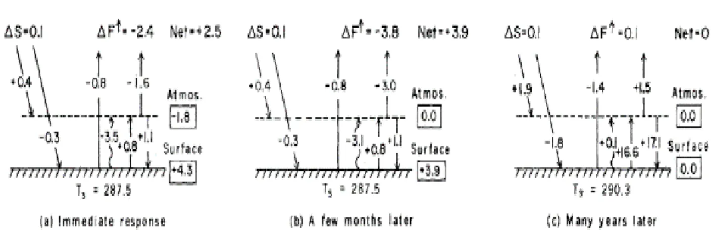
These timescales were made explicit by Hansen et al. (1981) who demonstrated the evolution of
672
the irradiance changes in their radiative-convective model, following a doubling of CO2 (see Fig.
673
2.1). This tracked the changes from: (i) the immediate response (nowadays called the
674
instantaneous RF (IRF)); (ii) the response after a few months (which is close to the RF
675
incorporating stratospheric temperature adjustment); in the case of a CO2 increase, the increased
676
emittance of the stratosphere leads to a cooling which increases the magnitude of the
677
perturbation of the top-of-atmosphere irradiance from -2.4 to -3.8 W m-2; and (iii) “Many years
678
later” when the surface temperature has equilibrated (following Expression (2.2)) and the
679
resulting irradiance change at the top of the atmosphere has cancelled out the forcing. Hansen et
680
al. (1981) seem to be the first to use the terminology “radiative forcing”, although they used it in
681
a general rather than a quantitative sense.
682
683
Several contributions to the edited volume by Clark (1982) also used the RF concept, at least in
684
an illustrative way, although using a variety of names. For example, Chamberlain et al. (1982)
685
compared different climate change mechanisms using what would now be called as surface
686
radiative forcing; their use of this (rather than tropopause or top-of-atmosphere RF) as a
687
predictor of surface temperature change was strongly disputed in the same volume by
688
Ramanathan (1982) (and earlier in Ramanathan et al., 1981), Hansen et al. (1982) and Luther
689
(1982). Hansen et al. (1982) briefly presented values of top-of-atmosphere radiative flux changes
690
for idealised changes in concentrations of 5 gases, and refer to these as “radiative forcings” in
691
their text. At around the same time, WMO (1982), in a brief report on a meeting on the potential
692
climate effects of ozone and other minor trace gases, refer explicitly to “the net outgoing
longwave flux at the tropopause” as determining “the radiative forcing of the surface-troposphere
694
system”, and present values for idealised perturbations of 6 greenhouse gases.
695
696
Ramanathan et al (1985) also used the term “radiative forcing” in the context of Expression
697
(2.2) and Dickinson and Cicerone (1986) appear to be the first to use the concept to quantify the
698
climate impact of changes in concentrations of several greenhouse gases relative to
pre-699
industrial times in W m-2 (using the term “trapping” rather than RF).
700
701
“Radiative forcing” became firmly established as accepted terminology in Chapter 15 of the
702
1985 WMO Ozone Assessment (WMO 1985) (which was largely reproduced in Ramanathan et
703
al. (1987)) and the term was widely used in their discussion; however, much of their overall
704
comparison of the impacts of climate forcing agents was still posed in terms of surface
705 temperature change. 706 707 708 709 710
2.3 The evolution of the radiative forcing concept during the IPCC era
711
712
Assessment of RF has been firmly embedded in IPCC assessments from it’s First Assessment
713
Report (FAR) onwards. FAR (Shine et al. 1990) took as its starting point the fact that the
714
climate impact of a range of different climate forcing agents could be compared using RF, in W
715
m-2, even though this was only starting to be done routinely in the wider literature at the time. A
716
significant motivator for the use of RF in all IPCC reports was as input to climate emissions
717
metrics (such as the Global Warming Potential, see Section 11). This section focuses mostly on
718
developments in understanding of anthropogenic forcings – more detailed discussions of the
719
evolution of the understanding of solar and volcanic aerosol forcings is given in Sections 8 and
720 9 respectively. 721 722 723 724
725
2.3.1 The IPCC First Assessment Report 1990 (FAR)
726 727 728
FAR discussed the concept of RF, stressing the utility of including stratospheric
729
temperature adjustment. Building on earlier work (e.g. Ramanathan et al. 1987) it also
730
emphasized the importance of indirect forcings, such as the impact of changes in methane
731
concentrations on ozone and stratospheric water vapor. The main focus was on greenhouse
732
gases, including extended tabulations of forcing due to CFCs and their potential replacements.
733
FAR also popularized the use of simplified expressions for calculating RF, which were
734
empirical fits to more complex model calculations. The expressions used in FAR were based on
735
two studies available at the time (Wigley et al. 1987; Hansen et al. 1988). Updated versions of
736
the simplified expressions are still widely used in simple climate models and for assessing
737
potential future scenarios of trace gas concentrations.
738
739
FAR also included, together in a single section, the roles of solar variability, direct aerosol
740
effects, indirect aerosol effects and changes in surface characteristics. The literature on these
741
was sparse. The section on direct aerosol forcing focused mostly on volcanic aerosol; it did not
742
attempt to quantify the impact of human activity because of “uncertainties in the sign, the
743
affected area and the temporal trend”. Perhaps surprisingly more attention was given to the
744
indirect aerosol effects (now more generally known as “aerosol cloud interactions”); although
745
FAR stated that “a confident assessment cannot be made”, due to important gaps in
746
understanding, a 1900-1985 estimate of -0.25 to -1.25 W m-2 (based on Wigley 1989) was
provided. FAR did not include estimates for pre-industrial to present-day RF across all forcing
748
agent, but restricted itself to two then-future periods (1990-2000 and 2000-2050).
749
750
Soon after FAR, an IPCC Supplementary Report provided an update (Isaksen et al. IPCC,
751
1992). Significant developments since FAR included more advanced RF estimates due to ozone
752
change (Lacis et al. 1990), and the first calculation of the forcing due to latitudinally-resolved
753
observed stratospheric ozone depletion (Ramaswamy et al., 1992). The indirect forcing due to
754
methane’s impact on tropospheric ozone and stratospheric water vapour were quantified. The
755
first geographically-resolved estimates of sulphate aerosol direct forcing (now referred to as
756
aerosol-radiation interaction ) (Charlson et al. 1991) had become available, indicating a
757
significant offset (in the global-mean sense) of greenhouse gas RF.
758
759
760
762
2.3.2 IPCC Special Report on Radiative Forcing and the IPCC Second Assessment Report
763
(SAR)
764 765
The SAR discussion on RF was partly based on the analysis of Shine et al. (1995) in an IPCC
766
Special Report. Since FAR there had been several important developments. The 1992 Pinatubo
767
volcanic eruption had allowed unprecedented global-scale observations of the impact of such a
768
large eruption on the radiation budget (Minnis et al. 1993) and the subsequent climate response
769
was well predicted (Hansen et al. 1993 updated in Shine et al. 1995); because of the transient
770
nature of the forcing, this still arguably constitutes the most direct evidence of the linkage
771
between transient forcing and transient response to date. Understanding of ozone RF continued
772
to develop as a result of ongoing analyses of observational data and the advent of (then 2-D,
773
latitude-height) chemistry models allowing improved estimates of the longer-term increases in
774
tropospheric ozone (e.g. Wang et al., 1993; Hauglustaine et al. (1994)). More sophisticated RF
775
calculations due to sulphate aerosol-radiation interaction were becoming available (e.g. Kiehl
776
and Briegleb, 1993; Hansen et al. 1993; Taylor and Penner 1994), as were the first climate
777
model simulations of aerosol cloud-interaction (Jones et al. 1994). Early attempts to estimate the
778
direct RF from biomass burning (Penner et al. 1992; Hansen et al. 1993) were presented. Shine
779
et al. (1994) produced the first of IPCC’s many figures of the pre-industrial to present-day
780
global-mean forcing incorporating both an estimate of the uncertainty range and a subjective
781
confidence level. Shine et al. (1994) also extended the discussion of the utility of the radiative
782
forcing concept; the chapter included clear demonstrations of the need to include stratospheric
783
temperature adjustment to compute ozone forcings, as IRF and RF could differ in sign.
784
Climate models were beginning to be used to test the forcing-response relationships for a wide
786
variety of forcings, including the impact of the spatial distribution of forcing; an unpublished
787
study by Hansen et al. (1993b) (a precursor to Hansen et al. (1997)) reported experiments with
788
an idealised GCM that indicated that extratropical forcings had almost double the impact on
789
global mean surface temperature change as the same (in the global-mean sense) tropical forcing;
790
ongoing work (e.g. Taylor and Penner 1994) also clearly demonstrated that while forcing in one
791
hemisphere was felt mostly in that hemisphere, there was still a large non-local response. By the
792
time of the SAR update (Schimel et al. 1996), attention had begun to focus on the (positive)
793
direct forcing due to soot (or black carbon) (Chylek and Wong 1995; Haywood and Shine 1995)
794
(see Section 5 for details), which highlighted the dependence of the computed forcing on
795
whether the aerosol population was internally or externally mixed. More studies of aerosol
796
indirect forcing were emerging (e.g. Boucher and Lohmann, 1995; Chuang et al, 1994) which
797
continued to indicate a significant negative forcing, as well as discussing indirect effects beyond
798
the impact on cloud effective radius. SAR updated the earlier RF figure most notably by
799
splitting the direct effect into its sulphate, biomass burning and soot components, but refrained
800
from giving a central estimate for the aerosol indirect forcing, “because quantitative
801
understanding of this process is so limited”.
802
803
805
2.3.3 IPCC Third Assessment Report (TAR)
806 807 808
After four IPCC reports with a focus on RF in the space of just 6 years, TAR’s analysis
809
(Ramaswamy et al. 2001) was able to assimilate developments over a much longer period, using
810
a much larger body of literature. This was particularly so for tropospheric ozone and aerosol
811
forcing, as a result of many more chemistry-transport and GCM studies. These included early
812
studies investigating mineral dust and nitrate aerosols. The sophistication and range of studies
813
on aerosol indirect forcing had increased, with much more effort to separate out first (droplet
814
radii) and second indirect (liquid water path) effects. The associated uncertainty in the first
815
indirect effect could not be reduced beyond that given in SAR; no estimate was given for the
816
second indirect effect because it was “difficult to define and quantify” but it was noted that it
817
“could be of similar magnitude compared to the first (indirect) effect”. Ramaswamy et al. (2001)
818
also reassessed the simple formulae used by IPCC to compute greenhouse gas RF, which led to
819
a 15% reduction in CO2 forcing relative to the FAR formula; this and subsequent reports mostly
820
adopted the expressions presented by Myhre et al. (1998).
821
822 823
TAR also included in its RF summary figure, for the first time, the effect of contrails and
824
contrail-induced cirrus, partly based on work presented in the IPCC Special Report on Aviation
825
and the Global Atmosphere (Prather et al. 1999) and the effect of land-use change on surface
826
albedo.
827
828
TAR continued the important discussion on the utility of the RF concept. A larger number of
829
GCM studies, with a more diverse set of forcing mechanisms, were available, leading to the
surface temperature response, but not to a quantitatively rigorous extent as in the case of …
832
radiative convective models”. Most notably, Hansen et al. (1997) had presented a wide-ranging
833
study with a simplified configuration of their climate model which examined the response to
834
both latitudinally and vertically constrained forcings. They showed that forcings confined to
835
specific altitudes could lead to specific cloud or lapse rate responses, and these resulted in
836
marked variations in climate sensitivity for a given forcing. This weakened the perception that
837
the global-mean climate sensitivity for spatially inhomogeneous forcings could be used to
838
determine quantitative aspects of the spatial responses. This important work also presaged later
839
developments in the definition of RF, and appears to be the first explicit usage of the concept of
840
“efficacy” (although it was not given that name) that is discussed in the next subsection.
841
842 843