Linear Logistic Test Modeling with R

Volume 20 Volume 20, 2015 Article 1 2015

Linear Logistic Test Modeling with R

Linear Logistic Test Modeling with R

Purya Baghaei

Klaus D. Kubinger

Follow this and additional works at: https://scholarworks.umass.edu/pare Recommended Citation

Recommended Citation

Baghaei, Purya and Kubinger, Klaus D. (2015) "Linear Logistic Test Modeling with R," Practical Assessment, Research, and Evaluation: Vol. 20 , Article 1.

DOI: https://doi.org/10.7275/8f33-hz58

Available at: https://scholarworks.umass.edu/pare/vol20/iss1/1

This Article is brought to you for free and open access by ScholarWorks@UMass Amherst. It has been accepted for inclusion in Practical Assessment, Research, and Evaluation by an authorized editor of ScholarWorks@UMass Amherst. For more information, please contact [email protected].

A peer-reviewed electronic journal.

Copyright is retained by the first or sole author, who grants right of first publication to the Practical Assessment, Research & Evaluation. Permission is granted to distribute this article for nonprofit, educational purposes if it is copied in its entirety and the journal is credited. PARE has the right to authorize third party reproduction of this article in print, electronic and database forms.

Volume 20, Number 1, January 2015 ISSN 1531-7714

Linear Logistic Test Modeling with R

Purya Baghaei, Islamic Azad University, Mashhad Branch, Mashhad, Iran

Klaus D. Kubinger, University of Vienna, Austria

The present paper gives a general introduction to the linear logistic test model (Fischer, 1973), an extension of the Rasch model with linear constraints on item parameters, along with eRm (an R package to estimate different types of Rasch models; Mair, Hatzinger, & Mair, 2014) functions to estimate the model and interpret its parameters. The applications of the model in test validation, hypothesis testing, cross-cultural studies of test bias, rule-based item generation, and investigating construct irrelevant factors which contribute to item difficulty are explained. The model is applied to an English as a foreign language reading comprehension test and the results are discussed.

An important aspect of validity theory is ‘explaining’ the mental processes that are triggered when test items are solved. This is in contrast to ‘prediction’ which is based on the correlation of tests with external criteria (Messick, 1989, Embretson, 1998). Understanding processes and cognitive operations (CO) which contribute to item difficulty has been given attention in cognitive psychology both for test validation and understanding learning processes. One common method that has been used for this purpose is regressing item difficulties (classical test theory p-values or Item Response Theory item difficulty estimates) on the frequency of cognitive components involved in solving the items. The other method is the estimation of the difficulty of cognitive operations as specified by the linear logistic test model (LLTM, Fischer, 1973; see also Fischer, 2005, and Kubinger, 2008, 2009).

LLTM is an extension of the Rasch model (RM, Rasch, 1980) which decomposes item parameters into a linear combination of several basic parameters that are defined a priori. The Rasch model is formally expressed as:

= 1 | ξ , ) = _{1 + exp ξ − )} exp ξ − )

where = 1 | ξ , )is the probability that person

v gives a correct response to item i, given her ability

ξ and the difficulty of item i as .

The LLTM imposes the following linear constraint on the difficulty parameter:

=

Where q_ijis the given weight of the basic parameter j on item i and η_j is the estimated difficulty of the basic parameter j.

The number of operations p is restricted to p<=k -1, where k is the number of items (Fischer, 2005). In other words, the item parameters σi is decomposed into

a weighted sum of basic parameters η_j

.

LLTM has also been extended to polytomous items with ordered response categories both for items with similar response categories (linear rating scale models) and for those with different response categories (linear partial credit models) (Fischer, 2005; Fischer & Ponocny-Seliger, 1998; Fischer & Ponocny, 1995). Nevertheless, the application of these models is rare.

Depending on the context of application n can be interpreted as the difficulty of the cognitive operations involved in solving the items or the contribution of each CO to item difficulty. q’s are the weights, that is the number of times we hypothesizes (a priori) a certain operation is needed to solve the item. In other cases where construct irrelevant factors such as item position effects (Hahne, 2008; Hohensinn, et al, 2008) or item format effects are modeled, η refers to these

difficulty. Under LLTM, CO difficulty estimates are independent of person ability estimates like in the Rasch model. Unidimensionality is required for LLTM and conditional likelihood estimation is available to estimate its parameters (Fischer, 1973/2005).

In laymen terms, LLTM assumes that the Rasch model item difficulty parameters are composed of the difficulty of several cognitive components or item characteristics which linearly add up and lead to the overall estimated difficulty parameter. According to Gorin (2005) characteristics of an item can be classified as radicals and incidentals. Radicals are substantive components of items which are responsible for their difficulty, i.e., characteristics which can be manipulated to change the cognitive processing needed to solve the item. Incidentals are surface characteristics which are not expected to affect item difficulty and the processing load of items. For example, in math word problems the names of objects and people are incidentals. LLTM helps us quantify the difficulty of radicals and incidentals, if we hypothesize those incidentals also affect difficulty.

The major motivation behind the development of LLTM was the need in educational settings to break down learning materials into smaller manageable units for learners to master (Fischer, 1973). Researchers for a long time have recognized the importance of quantitative parameterization of ‘learning quanta’ for optimal teaching and individual learning (Spada, 1972, cited in Fischer, 1973). To accomplish this goal, an academic subject, such as reading comprehension or algebra, should be systematically analyzed qualitatively and the basic learning units or cognitive operations which are needed to solve the pertinent test items derived. LLTM then parameterizes these units and tells us if they contribute significantly to the ‘true’ RM-based difficulty of items.

According to Fischer (1973) the strength of the model is in testing hypotheses that tell us which cognitive operations can be considered as psychological units. The model enables researchers to empirically test hypotheses about item solving processes and to establish substantive psychological theories. By identifying the cognitive processes which are needed to solve the items construct validity of items can be demonstrated and items for testing specific cognitive processes be written.

After estimating the difficulty of the learning units we should be able to reconstruct the RM-based difficulty of the items. Knowing which units are involved in solving the items we add up the difficulty of the units (multiplied by their weights) that are needed to solve the items. This LLTM-based difficulty estimates should approach the RM-based item difficulty parameters. The closer the LLTM-based difficulty parameters to RM-based difficulty parameters the better our construct theory, defined qualitatively in terms of the learning units, has accounted for the ‘true’ (RM-based) difficulty parameters. In case we cannot recover the RM-based difficulty estimates with the difficulty of the units we need to amend our theory by adding more units or revising the assignment of units to items. Furthermore, the fit of LLTM can be compared with the fit of the Rasch model to data by carrying out a likelihood ratio test.

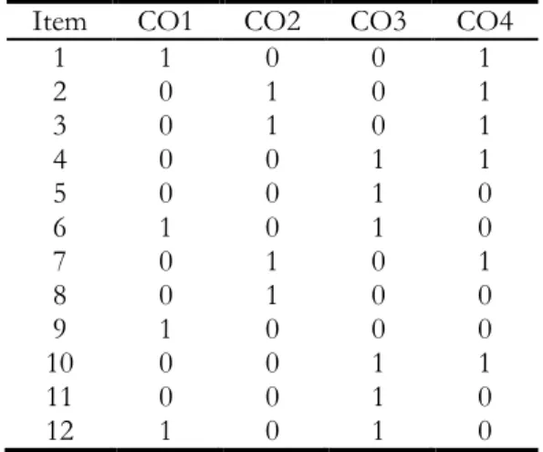
To apply LLTM to a test, which is the operationalization of a certain construct, content experts should specify the cognitive components or operations which are needed to solve the items. Then a Q-matrix ((qij)) needs to be defined. In the Q-matrix, content experts based on the theory of the construct decide on the weight of each cognitive operation in solving the items. Table 1 is the Q-matrix for an English as a second language reading comprehension test composed of 12 dichotomously scored items and four hypothesized cognitive operations.

Columns, CO1 to CO4 indicate the four cognitive operations tapped by the test. 0’s and 1’s are the given weights of the operations for each item. For instance, column CO1 shows that cognitive operation 1 is involved for answering items 1, 6, 9, and 12 each with a weight of 1. This operation has a weight of 0 for the other items, which means that it is not used to solve them. 0’s and 1’s indicate the presence or absence of the operation in solving the items. Alternatively weights of 2 and 3 or greater could have been given to the operations if content experts believed the operation is employed more than once for solving the item. In other words, the weight of a CO is the number of times the operation is involved in solving the item. Note that great care should be taken in specifying the Q-matrix as Q-matrix misspecification has profound effects on parameter estimates (Baker, 1993; Green & Smith, 1987; Macdonald, 2014).

Table 1: Q-matrix for a reading

comprehension test with four cognitive operations

Item CO1 CO2 CO3 CO4

1 1 0 0 1 2 0 1 0 1 3 0 1 0 1 4 0 0 1 1 5 0 0 1 0 6 1 0 1 0 7 0 1 0 1 8 0 1 0 0 9 1 0 0 0 10 0 0 1 1 11 0 0 1 0 12 1 0 1 0

A prerequisite for applying LLTM is that the standard Rasch model should hold for the data (Fischer, 1973). Fischer (2005) states that if the RM does not fit, at least approximately, there is no point in decomposing the item parameter because then the basic parameter and its estimator would lack an empirical meaning. Green and Smith (1987) suggest that before running LLTM one can delete persons and items that do not fit the assumptions of the Rasch model. In this way persons and items with alternative solution strategies are identified and can be removed.

The fit of the standard Rasch model is compared to the fit of LLTM using a likelihood ratio test. The deviance of -2 times log-likelihood of the two models is approximately chi-square distributed with degrees of freedom equal to the difference between the numbers of parameters in the two models (Fischer, 1973). Poor fit for LLTM results if all relevant COs are not modeled or the weights are not assigned correctly. In case of lack of fit the hypothesis can be improved and the model reapplied (Fischer, 2005). If RM does not fit significantly better than the LLTM then we have evidence of validity for the test in terms of the specified cognitive operations. If LLTM does not fit as good as the RM then the specified cognitive operations do not sufficiently account for the item difficulty parameters. This calls for revising the construct theory and our hypothesis about the structure of the construct in question and its underlying cognitive components. For validation purposes several competing Q-matrices can be defined and tested. However, looking for the best fit a-posterior always requires an independent

confirmation study. In an a-posterior model fit, it is possible that your model fits only the sample data and not the population. Thus you need an independent sample to test the new model as confirmation for the a-posterior fit (cf. “cross-validation” in Rasch, Kubinger, & Yanagida, 2011).

Previous applications in psychology and education

The earliest application of LLTM in education was by Fischer (1973). He analyzed a differential calculus test composed of 29 dichotomously scored items. Eight cognitive operations or rules were hypothesized to be involved in solving the items: (1) differentiation of a polynomial, (2) product rule, (3) quotient rule, (4) compound functions, (5) sin (x), (6) cos (x), (7) exp (x), and (8) ln (x). The difficulties of these eight operations were estimated with LLTM. Results showed that except for operations (2) and (7) the other operations significantly contributed to item difficulty estimates. It was also possible to reasonably reconstruct RM-based difficulty of the items with the difficulty of the hypothesized underlying operations. The correlation between RM-based and LLTM-based difficulty parameters was .87.

Kubinger (1979, 1980) investigated the elementary operations necessary to solve the items of a university statistics exam. The hypothesized elementary operations for this study included: understanding the measurement scale of the variable in question, checking normality of the data, checking whether the data are matched (paired), checking homogeneity of variances, etc. The purpose of the study was to identify more difficult operations to aid in modifying the teaching methods. Findings showed that the RM fitted the data significantly better than LLTM. This was interpreted as the failure of the theory (the elementary statistical operations) in accounting for item difficulties. The researcher concluded that there must be more factors involved in solving the items. When some other construct irrelevant factors such as the position of items in the booklet and the length of the item texts were considered LLTM fitted as good as the RM.

Along the same lines Sonnleitner (2008) tried to identify components of an item-generating system for reading comprehension in German as a first language. He identified eight radicals (e.g. propositional

complexity, degree of coherence, inference of causality, etc.) to explain reading item difficulty estimates. LLTM analyses showed that it was not possible to reconstruct item parameters by means of the cognitive operations and the textual features. When some response-related radicals such as the number of response options and the number of correct response options were taken into account LLTM sufficiently explained RM-based item parameters.

Embretson and Wetzel (1987) attempted to predicate the difficulty of multiple-choice (MC) paragraph comprehension items. They hypothesized that two major factors, namely, text characteristics and response decision factors contribute to item difficulty. Their model postulated that performance on MC reading comprehension items takes place in two stages: 1. text representation process, where the text is understood, and 2. decision process where item stem and alternatives are compared to text to select the correct alternative. In their model text factors included characteristic of the text to be read and comprehended including propositional density, argument density, percent of content words, etc. and response decision processes included falsification, confirmation, reasoning, etc. LLTM analysis of the data showed that both types of processes had significant impact on MC reading comprehension item difficulty estimates. They further demonstrated that decision process variables impacted item difficulty more that textual characteristics. That is, MC paragraph comprehension item difficulty parameters depend more on response decision than on text. They concluded that their MC items measure verbal and reasoning ability.

Zeuch, Holling, and Kuhn (2011) analysed the Latin Square Task (LST), a nonverbal measure of fluid intelligence, relational complexity and working memory (Birney, Halford, & Andrews, 2006). Each item consists of some cells, each containing a symbol. One cell is filled with a question mark. Test-takers have to select from a number of symbols which symbol fits the cell with the question mark. The rule is that every symbol must be used only once in every row or column. LST item difficulty is hypothesized to be governed by relational complexity (binary, ternary, quaternary), i.e., the number of rows and columns that are needed to be processed simultaneously to solve the item and the number of processing steps. It was hypothesized that the order of complexity of

operations from hardest to easiest is quaternary, ternary, binary, and the number of steps, respectively. LLTM calibration of processing operations confirmed the hypothesis. Quaternary relations turned out to be the most difficult operation followed by ternary, number of processing steps, and binary. They report a correlation coefficient of .85 between RM-based difficulty estimate and those recovered by LLTM.

Chen, MacDonald, and Leu (2011) used LLTM to investigate sources of item complexity in math fraction items. They identified six operations, namely, using illustrations, providing interpretations, applying judgment, computation, checking distractors, and solving routine problems underlying fraction conceptual items in a math fraction items given to a large sample of Taiwanese students (n=2612). LLTM showed that all six components significantly affect item difficulty, with applying judgment and providing interpretations as the hardest operations and routine problems and computation as the easiest. LLTM did not significantly fit better than the RM as is commonly reported by other researchers too. They attributed this to their large sample size and the sensitivity of the chi square test to large samples. Nevertheless, they found a substantially high correlation of .95 between LLTM-based item parameters and those estimated by the RM. To cross check the results of LLTM they regressed RM-based item difficulty estimates on the cognitive operations. Regression analysis showed that using illustrations and checking distractors did not significantly contribute to item difficulty. They argued that small sample (the number of items) in the regression analysis and low power was the reason why these two components turned out to be insignificant.

Another context where LLTM has been used is investigating item position effects. It is argued that in large scale assessments where, to prevent cheating, several test booklets (with the same items but in different item orders) are presented position effects may occur. Position effects are largely due to learning and fatigue. An item might be difficult if it is presented at the beginning of a test but easier if presented at the end due to the learning that takes place during the testing session. Or an item that is easy in the beginning might become hard if presented toward the end of the test booklet due to examinee fatigue. If all examinees take the same items in the same order these effects are

equal for all and are not a cause for concern as position effect is balanced for all examinees. However, in other contexts where the order of items changes (e.g. in large scale testing or computer adaptive testing) item difficulty parameters contain an unknown component due to their position in the test which could lead to unfair examinee comparisons. This could happen because an examinee might be advantaged or disadvantaged by encountering a specific item at a certain position (Hohensinn, et al., 2008).

For investigating position effects or the effects of any other experimental condition with LLTM each position/condition should be considered a “cognitive operation” and each item is parameterized separately in each position. Therefore, there will be virtual items, the number of which is equal to the number of actual items multiplied by the number of positions. The difficulty of each virtual item is assumed to be a linear combination of the content of the item and the effect of the position of the item within the test booklet (Hohensinn, et al. 2008; Kubinger, 2008/2009). Rather than representing the difficulty of cognitive operations basic parameters in such designs show the change of item difficulty under each experimental condition. Hohensinn, et al. (2008) investigated position effects in a large scale mathematics competence test and discovered a small fatigue effect. However, Hahne (2008) investigated position effects in Viennese Matrices Test (Formann & Piswanger, 1979) which was presented in six different orders and found no position effect for this test.

Despite being a very powerful model in understanding the cognitive processes underlying test performance and providing validity evidence, LLTM has not received enough attention in cognitive psychology and education. The following section provides detailed explanations on how to estimate the model using eRm package (Mair, Hatzinger, & Mair, 2014) and interpret the output.

Estimating LLTM with eRm package in R

In this section LLTM is applied to an English as a foreign language reading comprehension test composed of 12 dichotomously scored items. The test is a section of a national high stakes test for admitting candidates to PhD programmes at Tehran University. A section of the data (n=1550) is selected for analysis. The Q-matrix for the 12 items, presented above in Figure 1, was drawn up by the authors for this analysis.

LLTM can be estimated with eRm package (Mair, Hatzinger, & Mair, 2014) in R, free open source software. Below eRm functions for running LLTM and the interpretation of the output are explained. More details about the applications are presented afterwards.

> library(eRm) # eRm package is loaded.

>

setwd("C:\\Users\\Baghaei\\Documents\\R-Analyses")# specify the folder where the data

file is. Note that back slashes should be doubled.

>

data<-read.table("Reading-lltm.dat",header=TRUE)# the data file is

specified.

> data1<-data [,1:12] # columns of items in the

data file are specified.

> res <-RM(data1) # the standard Rasch model is

estimated.

> summary(res) #gives the results of RM estimation:

(see Table 2)

Table 2: RM Results

The table above shows the RM item easiness1

parameter estimates for the 12 items along with their standard errors and their 95% confidence intervals.

> fit<-LRtest(res, splitcr = "mean" , se =

TRUE) # fit of RM according to Andersen’s (1973)

likelihood ratio test with the mean of raw scores as the partitioning criterion is assessed.

1 _{Note that eRm package estimates easiness parameters for} LLTM instead of difficulty parameters. Easiness parameters have opposite signs to difficulty parameters. Since the signs are arbitrary, reverse the signs if you are more used to difficulty parameters.

The result is:

Andersen LR-test: LR-value: 12.603 Chi-square df: 11 p-value: 0.32

The p-value shows that the likelihood ratio test is non-significant and, therefore, the RM holds for the data. In the next step, LLTM is estimated.

> q.ij<-matrix(c(1, 0, 0, 0, 0, 1, 0, 0, 1, 0, 0, 1,

+ 0, 1, 1, 0, 0, 0, 1, 1, 0, 0, 0, 0, + 0, 0, 0, 1, 1, 1, 0, 0, 0, 1, 1, 1, + 1, 1, 1, 1, 0, 0, 1, 0, 0, 1, 0, 0),

+ ncol=4) # the Q-matrix presented in

Table 1 is assigned to the object ‘q.ij’ using the function ‘matrix’.

> Reading.LLTM <- LLTM(data1, q.ij) # LLTM

function is applied to data1 and the Q-matrix we named ‘q.ij’.

> summary (Reading.LLTM) # gives the results of

LLTM estimation (see Table 3)

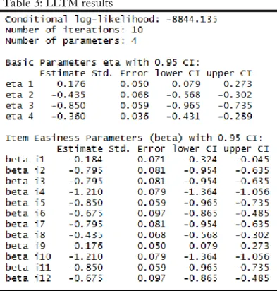
Table 3 shows the easiness of the four cognitive operations or basic parameters (eta 1 to eta 4) as well as their standard errors and 95% confidence intervals. For easier interpretation of the basic parameters we can change them to difficulty parameters by reversing their signs. Operations with negative difficulty parameters (positive easiness parameters), such as CO1, make items easier but COs with positive difficulty parameters (negative easiness parameters) make them more difficult. The most difficult CO to master is CO3 with an estimated difficulty parameter (eta) of .85. Additionally, the 95% confidence interval reported for each eta parameter shows whether the parameter is significantly different from zero or not. Parameters whose confidence intervals do not include zero are significant. In this study all eta parameters are significantly different from zero (p < .05). Bear, however, in mind that using some likelihood ratio test for testing specifically a certain null hypothesis with respect to a certain CO (or even all of them) means a study-wise (type-I) risk. Using confidence intervals entails only to analyze with a comparison-wise risk so that the study-wise risk is in most cases quite larger than the nominal type-I-risk a_{, but actually unknown}

(cf. Rasch, Kubinger, & Yanagida, 2011).

Table 3: LLTM results

In an LLTM analysis of a math test with eight basic operations, Fischer (1973) found that some of the operations had negative difficulty parameters. Since this was unexpected and theoretically unjustifiable he concluded that the construct model defined in terms of the Q-matrix was inadequate. He discovered that the operations which were found more than once in many items (i.e. had weights greater than 1) had negative difficulty parameters. Fischer suggested that in the context of that math test testees who once mastered a specific rule (basic operation) the number of times this rule had to be applied within an item was of no relevance and hence does not contribute to difficulty. Therefore, he defined another Q-matrix with weights of only 1’s and 0’s and reanalyzed the data and got positive difficulty parameters for all the operations. Nevertheless, Kubinger (1979, 1981) showed that when COs are weighted by the number of times the respective rule is applied within an item LLTM fits and the difficulty parameters of COs (eta) are positive.

The second part of Table 2 shows the LLTM item easiness parameters, based on the CO parameters. We stated that in LLTM we hypothesize that item difficulties are a linear combination of several basic parameters (eta). For example, for solving item 1 cognitive operation 1 and 4 are involved. The difficulty estimates of these two operations are 0.176 and -0.360,

respectively. The LLTM item easiness estimate for this item is (0.176-0.360) =-0.184. For solving item 2 operations 2 and 4 with easiness parameters of -0.435 and -0.360, respectively are required. The LLTM easiness estimate for item 2 is (– 0.435-0.360) =-0.795. Therefore, we see that LLTM item estimates are computed by adding the easiness estimates of the operations needed to solve them. When a basic operation has a weight greater than 1, the basic parameter η should first be multiplied by its corresponding weight before summing up. Since here all COs have a weight of 1 we did not need to do that.

The next step is comparing LLTM item easiness parameters with the RM item easiness parameters. The closer the RM easiness parameters are to the LLTM easiness parameters the better our construct theory, which is formulated in terms of cognitive operations in the Q-matrix, has accounted for item parameters. In other words, with the cognitive operations we try to recover the RM item parameters. This is more or less similar to regressing RM item difficulty parameters on cognitive operations trying to predict item parameters with a number of predictors which are CO’s here (Green & Smith, 1987; Scheiblechner, 1972).

However, Embretson and Daniel (2008) demonstrate that regression modeling of item difficulties lead to less clear interpretations of the relative impact of CO’s since they have large standard errors and the parameters estimated for them cannot be used for item banking because they are inconsistent and biased. We expect item parameters reproduced from LLTM to be the same as those estimated by the RM except for random errors (Fischer, 1973, 2005). To compare item parameters across the two models we can plot the item parameter estimations based on the respective models against each other. Before that we have to normalize the item easiness parameters based on the CO-parameters to a sum of zero:

>

betapar.lltm<-Reading.LLTM$betapar-mean(Reading.LLTM$betapar) # we subtract

the mean of the item easiness parameters based on the CO parameters from each item parameter in order to normalize them to sum to zero.

Then we can do the plotting:

> plot(res$betapar, betapar.lltm, xlim = c(-4, 4), ylim = c(-4, 4),xlab = "Item Easiness Parameter-RM",ylab = "Item

Easiness Parameter-LLTM") # RM item

parameters are plotted against LLTM item parameters.

The abscissa is labeled “Item easiness Parameter-RM" and the ordinate is labeled "Item Easiness ParameterLLTM". The scales of the axes range from -4 to -4. We additionally like to fit in the -45-degree line, which would represent all points in the Cartesian system when LLTM and RM completely coincide:

> abline(0,1) # gives the 45-degree line.

The plot shows that there is some concurrence, but some items’ difficulties are not explained exactly by our LLTM hypothesis. To compare item parameters across the two models we could also correlate them.

> cor(res$betapar, Reading.LLTM$betapar)#

computes the correlation coefficient between RM and LLTM easiness parameters.

Which returns:

[1] 0.5840389

The correlation coefficient between the two sets of item parameters is 0.584 which is rather small. This means that only (0.5842_{×100) 34% of the variance in}

RM item parameters can be accounted for by the four cognitive operations we defined. That is, readers firmly established in traditional correlational analysis might conclude that our construct theory has failed and needs to be amended. However, those grounded in IRT will prefer some likelihood ratio test in order to decide whether LLTM does explain the data as well as the Rasch model. Of course, any correlation coefficient depends on the range of the characters’ values, too; in our case this leads to a rather small coefficient, but the literature proves that for LLTM the correlation coefficients comes rather close to one, in most cases

(e.g. Kubinger, 1979, 1981; Hohensinn et al., 2008). Hence we have to look for such a likelihood ratio test.

We stated above that the difference between

likelihoods of the two models is approximately chi square distributed with the difference between the numbers of parameters as degrees of freedom. The

above outputs show that the log-likelihood of the RM

and LLTM are -8290.033 and -8844.135, respectively.

Therefore, -2log-likelihoods of the models are 16580.066 and 17688.27, respectively. The RM has a

smaller -2log-likelihood and, therefore, has a better fit as expected because RM uses more parameters.

In eRm we can execute:

> 2*(res$loglik - Reading.LLTM$loglik)

difference in -2log-likelihoods of the models are

computed. Which returns:

[1] 1108.203

> res$npar-Reading.LLTM$npar# the

the numbers of estimated parameters in the two models are computed to have the associated

degrees of freedom. Which returns:

[1] 7

> qchisq (0.95, df = 7)# gives the 0.95 quantile

(α=0.05) of the χ2 distribution with df

Which returns:

[1] 14.06714

The resulting value of the (asymptotically) chi square distributed statistic is much greater than the

critical value; therefore, the null-hypothesis (there is no difference in data’s likelihood for the models) must be rejected. The Rasch model fits the dat

better than the LLTM. This means that our reading theory defined in terms of the four cognitive operations is not satisfactory and has failed to account for (all) the item parameters. We could now look for construct

irrelevant factors such as item position effect or test format to account for the RM item difficulties.

Q-matrix (mis)specification

Correct specification of the Q-matrix is the most important factor in successful LLTM analysis. There are some general points about building the Q

(e.g. Kubinger, 1979, 1981; Hohensinn et al., 2008). Hence we have to look for such a likelihood ratio test.

We stated above that the difference between

-2log-of the two models is approximately chi

-square distributed with the difference between the numbers of parameters as degrees of freedom. The likelihood of the RM 8844.135, respectively. likelihoods of the models are 16580.066 and 17688.27, respectively. The RM has a likelihood and, therefore, has a better fit as expected because RM uses more parameters.

Reading.LLTM$loglik) # the

likelihoods of the models are

# the difference in

of estimated parameters in the two models are computed to have the associated

# gives the 0.95 quantile

df=7.

The resulting value of the (asymptotically) chi

-square distributed statistic is much greater than the hypothesis (there is no difference in data’s likelihood for the models) must be rejected. The Rasch model fits the data significantly

better than the LLTM. This means that our reading theory defined in terms of the four cognitive operations is not satisfactory and has failed to account for (all) the item parameters. We could now look for construct as item position effect or test format to account for the RM item difficulties.

matrix (mis)specification

matrix is the most important factor in successful LLTM analysis. There are some general points about building the Q-matrix

and some more specific ones. The first point is that there must be some overlap in the items in terms of cognitive operations. Consider a test composed of 20 items measuring four cognitive operations. The 20 items are divided into four blocks, each

items. Further suppose that each block of items measures a separate cognitive operation. Therefore, there is no connection among the items in terms of cognitive operations. Such a Q

facilitate parameter estimation. Q

designed in such a way that some items measure at least two operations so that the design gets connected. However, note that operations which are shared by all items are not estimable either and should be removed.

The other issue is a matter of c

matrix might be misspecified as assignment of operations to items is poor or even wrong. For instance, a teacher might specify that a particular CO is tapped by an item when in reality it is not. Or a teacher might argue that a certain CO is

answering an item when it is. Since assignment of weights is a completely subjective process and is done by teachers or other content experts great care should be taken by content experts in assigning CO’s to items.

Usually group consensus and discussions are required for correct allocation of weights to items and approval

of the final Q-matrix. Wrong assignment of weights to CO’s can lead to biased estimates of basic parameters. Furthermore, for correct estimation of

cognitive operation must be tapped by a sufficient number of items (Baker, 1993).

Baker (1993) using a simulation study demonstrated that misspecification of the weights lead to high root mean squares for

problem exacerbates when the Q

spars Q-matrix many of the cells are 0’s while in a dense matrix many of the cells contain 1’s. In other words, the relative number of CO’s tapped by the items

has an impact on the correct estimation of the basic parameters. Baker (1993) argues that “In a dense Q matrix, a larger number of cognitive operations are involved in each item and a low level of misspecification tends to get “smoothed out” over the

test items. Because of this, the consequences of a low level of misspecification were not quite as serious in the dense matrix condition as they were in the sparse matrix condition” (p.208). He also indicates that and some more specific ones. The first point is that there must be some overlap in the items in terms of cognitive operations. Consider a test composed of 20 items measuring four cognitive operations. The 20 items are divided into four blocks, each having five

items. Further suppose that each block of items measures a separate cognitive operation. Therefore, there is no connection among the items in terms of cognitive operations. Such a Q-matrix does not

facilitate parameter estimation. Q-matrixes should be

designed in such a way that some items measure at least two operations so that the design gets connected. However, note that operations which are shared by all items are not estimable either and should be removed.

The other issue is a matter of content. The

Q-matrix might be misspecified as assignment of operations to items is poor or even wrong. For instance, a teacher might specify that a particular CO is tapped by an item when in reality it is not. Or a teacher might argue that a certain CO is not involved in

answering an item when it is. Since assignment of weights is a completely subjective process and is done by teachers or other content experts great care should be taken by content experts in assigning CO’s to items. and discussions are required for correct allocation of weights to items and approval matrix. Wrong assignment of weights to CO’s can lead to biased estimates of basic parameters. Furthermore, for correct estimation of η parameters a

e operation must be tapped by a sufficient number of items (Baker, 1993).

Baker (1993) using a simulation study demonstrated that misspecification of the weights lead to high root mean squares for and η parameters. The

problem exacerbates when the Q-matrix is sparse. In a

matrix many of the cells are 0’s while in a dense matrix many of the cells contain 1’s. In other words, the relative number of CO’s tapped by the items ect estimation of the basic parameters. Baker (1993) argues that “In a dense Q matrix, a larger number of cognitive operations are involved in each item and a low level of misspecification tends to get “smoothed out” over the he consequences of a low level of misspecification were not quite as serious in the dense matrix condition as they were in the sparse matrix condition” (p.208). He also indicates that

sample size has a small impact on the estimation. For correct estimation of basic parameter we need a minimum number of test takers correctly answering to the items which tap the pertinent CO’s. When Q-matrix is sparse in order to get enough data for each CO a large sample size is required.

Summary and Conclusion

In this paper linear logistic test model (Fischer, 1973) and its applications in cognitive psychology and education was illustrated. The contribution of the model to investigating construct validity is demonstrated. Furthermore, eRm functions to estimate the model and interpret the output are given.

Baker (1993) states that LLTM bridges the gap between cognitive science and psychometrics. Disclosing the mental processes which produce the reliable variance is at the heart of construct validity (Baghaei, 2009). Identifying the components which make items difficult help explicate the construct validity of tests and disclose what they really measure. LLTM provides substantive insights into the structure of item difficulty and examinees’ cognitive solution strategies which in turn lead to more efficient item development. This provides a systematic method of validation at the item level.

Ascertaining the substantive aspect of construct validity (Messick, 1989) or Embretson’s (1998) construct representation validity necessitates identifying the processes that test-takers are engaged in when solving the items. Adequate fit of LLTM supports the substantive aspect of construct validity (Messick, 1989) and construct representation validity (Embretson & Daniel, 2008). Furthermore, items whose difficulty parameters cannot be reasonably reproduced by LLTM provide valuable information about the construct theory and call for reformulating the basic operations.

With LLTM new items with known item difficulty parameters can be constructed without administering them to estimate their difficulties (Fischer & Pendl, 1980). This is possible when the difficulty of the basic operations which contribute to item difficulty is known. Once we know the difficulty of the basic parameters, the difficulty of items which have unique combinations of the estimated cognitive components can easily be predicted. This is particularly helpful in item banking and adaptive testing. This application necessitates the

stability of the basic parameter estimates across populations. Studies of Piswanger (1975), Nährer (1977), and Habon (1981) in the context of Viennese Matrixes Test (a nonverbal intelligence test, Formann & Piswagner, 1979) show that basic parameters remain, more or less, stable across populations (cited from Fischer & Formann, 1982). The model can also be used in monitoring learning processes by applying it at different time points in the course of a programme or year to monitor the effect of training and teaching programmes on the difficulty of the basic parameters (Fischer, 1973).

Based on these results, we can generally conclude that a specific application of LLTM is cross-cultural examination of basic parameters; by this means one could explicate differential item functioning (DIF) at a more substantive level (cf. Tanzer, Gittler, & Ellis, 1995). Again, the null-hypothesis that the basic parameters are equal in the two populations can be tested against the alternative hypothesis that they differ by means of a Likelihood Ratio-test.

But of course there are other topics that LLTM can address. Kubinger (2008, 2009) exemplified, how several item administration effects could be tested: a) Rasch model item calibration using data sampled consecutively in time but partly from the same examinees; b) measuring position effects of item presentation, in particular, learning and fatigue effects – specific for each position, linear or non-linear; c) measuring content-specific learning effects; d) measuring warming-up effects; e) measuring effects of speeded item presentation; f) measuring effects of different item response formats.

Applying LLTM is not without limitations and problems, though. Green and Smith (1987) enumerate LLTM limitations: First, it is not possible to include all the cognitive operations which are involved in problem solving in the model and one runs the risk of focusing on observable aspects of the items instead of the actual processes and strategies that examinees use to arrive at the solutions. Second, the model assumes that the difficulty of the items is the linear combination of CO difficulties. This assumption may not be warranted in light of our knowledge of CO’s for solving items. And third, the model assumes that the same CO’s are used by all examinees, while different examinees may use different ways to arrive at the solutions. “Given these

constraints we suggest that it is still useful to develop a component equation that can be used to predict the difficulty of items. This is particularly true in those cases in which the items can be thought of as consisting of a small number of components” (Green & Smith, 1987, p. 372).

A common observation in the application of LLTM is that the model most often does not fit the data (according to the likelihood ratio test). This frequently happens when it is applied to existing tests rather than those developed on the basis of a cognitive model. Even Fischer and Formann (1982) argue that such statistical significance tests should not be overrated as large samples and few parameters are used to test the hypotheses, i.e., the tests are rather powerful. The more relevant factor when applying LLTM is whether the basic parameters are consistent enough across populations and items and useful for test construction purposes and development of cognitive theories. “Even in cases of an unsatisfactory conformity of the model to the data, the mere formulation of those hypotheses which are needed for working with the LLTM leads to a clearer understanding of the substantive problems” (Fischer & Formann, 1982, p. 412). And “Nevertheless, item difficulty could often be explained approximately” (Fischer, 2005, p.511).

References

Andersen, E. B. (1973). A goodness of fit test for the Rasch model. Psychometrika, 38, 123-140.

Baghaei, P. (2009). Understanding the Rasch model. Mashhad: Mashhad Islamic Azad University Press.

Baker, F. (1993). Sensitivity of the linear logistic test model to misspecification of the weight matrix. Applied Psychological Measurement, 17, 201-210.

Birney, D. P., Halford, G. S., & Andrews, G. (2006). Measuring the influence of complexity on relational reasoning. The development of the Latin Square Task. Educational and Psychological Measurement, 66, 146 − 171. Chen, Y.-H., MacDonald, G., & Leu, Y.-C. (2011).

Validating cognitive sources of mathematics item difficulty: Application of the LLTM to fraction conceptual items. The International Journal of Educational and Psychological Assessment, 7, 74-93.

Embretson, S. E., & Daniel, R. C. (2008). Understanding and quantifying cognitive complexity level in

mathematical problem solving items. Psychology Science Quarterly, 50, 328-344.

Embretson, S. E. (1998). A cognitive design system approach to generating valid tests: Application to abstract reasoning. Psychological Methods, 3, 380-396. Embretson, S. E., & Wetzel, C. D. (1987). Component

latent trait models for paragraph comprehension tests. Applied Psychological Measurement, 11, 175-193.

Fischer, G. H. (1973). The linear logistic test model as an instrument in educational research. Acta Psychologica, 37, 359-374.

Fischer, G.H. (2005). Linear logistic test models. In

Encyclopedia of Social Measurement, 2, 505-514.Fischer, G. H., & Formann, A. K. (1982). Some applications of logistic latent trait models with linear constraints on the parameters. Applied Psychological Measurement. 4, 397-416. Fischer, G. H., & Ponocny-Seliger, E. (1998). Structural Rasch

modeling: Handbook of the usage of LPCM-WIN 1.0. ProGAMMA, Groningen, The Netherlands.

Fischer, G. H., & Ponocny, I. (1995). Extended rating scale and partial credit models for assessing change. In Fischer, G.H. & Molenaar, I.W. (Eds). Rasch Models: Foundations, Recent Developments, and Applications (pp. 69-95). Springer-Verlag, New York.

Fischer, G. H., & Pendl, P. (1980). Individualized testing on the basis of the dichotomous Rasch model. In L. J.Th. van der Kamp, W. F. Langerak, & D. N. M.de Gruijter (Eds.), Psychometrics for educational debates (pp. 171-187). New York: Wiley.

Formann, A. K., & Piswanger, K. (1979). Wiener Matrizen Test. Ein Rasch-skalierter sprachfreier Intelligenztest [Vienese Matrixes Test: A nonverbal intelligence test scaled with the Rasch model]. Weinheim: Beltz Test. Gorin, J. S. (2005). Manipulating Processing Difficulty of

Reading Comprehension Questions: The Feasibility of Verbal Item Generation. Journal of Educational

Measurement, 42, 351-373.

Green, K.E., & Smith, R. M. (1987). A comparison of two methods of decomposing item difficulties. Journal of Educational Statistics, 12, 369-381.

Hahne, J. (2008). Analyzing position effects within reasoning items using the LLTM for structurally incomplete data. Psychology Science Quarterly, 50, 379-390.

Hohensinn, C., Kubinger, K. D., Reif, M., Holocher-Ertl, S., Khorramdel, L., & Frebort, M. (2008). Examining item-position effects in large-scale assessment using the Linear Logistic Test Model. Psychology Science Quarterly, 50, 391-402.

Kubinger, K.D. (1979). Das Problemlöseverhalten bei der statistischen Auswertung psychologischer Experimente. Ein Beispiel hochschuldidaktischer Forschung

tasks. An example of didactics research in higher education]. Zeitschrift für Experimentelle und Angewandte Psychologie, 26, 467-495.

Kubinger, K.D. (1980). Die Bestimmung der Effektivität universitärer Lehre unter Verwendung des Linearen Logistischen Testmodells von Fischer. Neue Ergebnisse [Evaluation of university teaching’s efficiency using Fischer’s linear logistic test model – Some new results]. Archiv für Psychologie, 133, 69-79. Kubinger, K. D. (2008). On the revival of the Rasch-model

based LLTM: From constructing tests using item generating rules to measuring item administration effects. Psychological Science Quarterly, 50, 311-327. Kubinger, K. D. (2009). Applications of the linear logistic

test model in psychometric research. Educational and Psychological Measurement, 69, 232-244.

Kubinger, K.D., Rasch, D. & Yanagida, T. (2009). On designing data-sampling for Rasch model calibrating an achievement test. Psychology Science Quarterly, 51, 370-384. Kubinger, K.D., Rasch, D. & Yanagida, T. (2011). A new

approach for testing the Rasch model. Educational Research and Evaluation, 17, 321-333.

Macdonald, G.C. (2014). The performance of the linear logistic test model when the Q-matrix is misspecified: A simulation study. Graduate Theses and Dissertations.

http://scholarcommons.usf.edu/etd/5065.

Mair, P., Hatzinger, R., & Mair, M. J. (2014). eRm: extended Rasch modeling [Computer software]. R package version 0.15-4. http://CRAN.R-project.org/package=eRm. R CORE TEAM. (2012). R: a language and environment for

statistical computing [Computer program]. Vienna,

Austria: R Foundation for Statistical Computing. ISBN 3-900051-07-0, URL http://www.R-project.org/. Rasch, G. (1980). Probabilistic models for some intelligence and attainment tests. Expanded ed. University of Chicago Press, Chicago, IL. (Originally published 1960, Pædagogiske Institut, Copenhagen.)

Rasch, D., Kubinger, K.D. & Yanagida, T. (2011). Statistics in Psychology Using R and SPSS. Chichester: Wiley.

Scheiblechner, H. (1972). Das Lernen und Lösen komplexer Denkaufgaben. Zeitschrift für Experimentelle und

Angewandte Psychologie, 19, 476-506.

Sonnleitner, P. (2008). Using the LLTM to evaluate an item-generating system for reading

comprehension. Psychology Science Quarterly, 50, 345-362. Tanzer, N. K., Gittler, G., & Ellis, B. B. (1995).

Cross-cultural validation of item

complexity in an LLTM-calibrated spatial ability test. European Journal of Psychological Assessment, 11, 170-183. Zeuch, N., Holling, H., & Kuhn, J.T. (2011). Analysis of the

Latin Square Task with linear logistic test models. Learning and Individual Differences, 21, 629-632.

Acknowledgment:

The work of the first author is supported by the Österreichische Austauschdienst (Austrian Exchange Service), Ernst Mach Grant.

Citation:

Baghaei, Purya & Kubinger, Klaus D. (2015). Linear Logistic Test Modeling with R. Practical Assessment, Research & Evaluation, 20(1). Available online: http://pareonline.net/getvn.asp?v=20&n=1

Corresponding Author:

Purya Baghaei English Department Islamic Azad University Ostad Yusofi St.

91871-Mashhad, Iran Pbaghaei [at] Mshdiau.ac.ir