Testing the predictability and efficiency of securitized real estate markets

econ

stor

www.econstor.eu

Der Open-Access-Publikationsserver der ZBW – Leibniz-Informationszentrum Wirtschaft

The Open Access Publication Server of the ZBW – Leibniz Information Centre for Economics

Nutzungsbedingungen:

Die ZBW räumt Ihnen als Nutzerin/Nutzer das unentgeltliche, räumlich unbeschränkte und zeitlich auf die Dauer des Schutzrechts beschränkte einfache Recht ein, das ausgewählte Werk im Rahmen der unter

→ http://www.econstor.eu/dspace/Nutzungsbedingungen nachzulesenden vollständigen Nutzungsbedingungen zu vervielfältigen, mit denen die Nutzerin/der Nutzer sich durch die erste Nutzung einverstanden erklärt.

Terms of use:

The ZBW grants you, the user, the non-exclusive right to use the selected work free of charge, territorially unrestricted and within the time limit of the term of the property rights according to the terms specified at

→ http://www.econstor.eu/dspace/Nutzungsbedingungen By the first use of the selected work the user agrees and declares to comply with these terms of use.

Schindler, Felix; Rottke, Nico; Füss, Roland

Working Paper

Testing the predictability and efficiency

of securitized real estate markets

ZEW Discussion Papers, No. 09-054 Provided in cooperation with:

Zentrum für Europäische Wirtschaftsforschung (ZEW)

Suggested citation: Schindler, Felix; Rottke, Nico; Füss, Roland (2009) : Testing the predictability and efficiency of securitized real estate markets, ZEW Discussion Papers, No. 09-054, http://hdl.handle.net/10419/28115

Dis cus si on Paper No. 09-054

Testing the Predictability and Efficiency

of Securitized Real Estate Markets

Dis cus si on Paper No. 09-054

Testing the Predictability and Efficiency

of Securitized Real Estate Markets

Felix Schindler, Nico Rottke, and Roland Füss

Die Dis cus si on Pape rs die nen einer mög lichst schnel len Ver brei tung von neue ren For schungs arbei ten des ZEW. Die Bei trä ge lie gen in allei ni ger Ver ant wor tung

der Auto ren und stel len nicht not wen di ger wei se die Mei nung des ZEW dar.

Dis cus si on Papers are inten ded to make results of ZEW research prompt ly avai la ble to other eco no mists in order to encou ra ge dis cus si on and sug gesti ons for revi si ons. The aut hors are sole ly

respon si ble for the con tents which do not neces sa ri ly repre sent the opi ni on of the ZEW. Download this ZEW Discussion Paper from our ftp server:

Non-technical Summary

Since the early 1970s and the seminal papers of Fama (1965, 1970), the efficient market hypothesis and its validity for several asset markets have been the topic of an uncountable number of publications in finance. The efficient market hypothesis deals with the question whether stock prices fully reflect all information available at a specific point in time. Weak-form tests of the efficient market hypothesis focus on the inWeak-formation set of historical prices or return series.

Today, there is abundant empirical evidence that stock markets are efficient, at least in its weak form. This means that investors are not able to earn excess returns compared to a buy-and-hold strategy by developing and using trading strategies. In contrast, the validity of the efficient market hypothesis is analyzed in less detail for international securitized real estate stock markets, and the few studies that exist focus mainly on the US-market.

Thus, this paper examines the behavior of securitized real estate returns for 14 countries over the period from January 1990 to December 2006. The parametric test results indicate that the random walk hypothesis is rejected for several markets. However, since the rejection of the

random walk hypothesis does not necessarily imply market inefficiency, a non-parametric

technique to test for market efficiency is also conducted. Additionally, the practical relevance of rejecting the random walk hypothesis is tested by implementing trading strategies based on moving averages.

Empirical evidence shows that the return generating process of the major securitized real estate markets differs significantly from the theoretical model of a random walk. The empirical findings of return predictability suggest that investors are likely to earn excess returns by using past information in most of the public real estate markets. Trading strategies based on moving averages allowing them to earn risk-adjusted excess returns are compared to a buy-and-hold strategy.

Das Wichtigste in Kürze

Spätestens seit den 70er Jahren und den frühen Arbeiten von Fama (1965, 1970) ist die Hypothese effizienter Märkte und die Überprüfung ihrer Gültigkeit für diverse Wertpapiermärkte in der Finanzwirtschaft Gegenstand einer nahezu unerschöpflichen Anzahl von Forschungsarbeiten. Die Hypothese effizienter Märkte beschäftigt sich mit der Frage, ob Wertpapierpreise alle zu einem bestimmten Zeitpunkt verfügbaren Informationen vollständig widerspiegeln. Dabei konzentriert sich die Überprüfung schwach-effizienter Märkte auf die Informationsmenge von historischen Preisen und Renditen.

In der Wissenschaft besteht heute weitgehend Einigkeit darüber, dass die Aktienmärkte zumindest als schwach-informationseffizient bezeichnet werden können und es Anlegern daher nicht möglich ist, durch Handelsstrategien gegenüber einer Buy-and-Hold-Strategie Überrenditen zu erzielen. Dagegen ist die Gültigkeit der Hypothese effizienter Märkte für die internationalen Immobilienaktienmärkte weitaus weniger intensiv analysiert worden, wobei sich die wenigen existierenden Untersuchungen auf diesem Gebiet im Wesentlichen auf den US-amerikanischen Markt konzentrieren.

Dieser Aufsatz untersucht daher das Renditeverhalten an 14 internationalen Immobilienaktienmärkten über einen Zeitraum von Januar 1990 bis Dezember 2006. Da sowohl parametrische als auch nicht-parametrische Testverfahren die Gültigkeit der Random-Walk-Hypothese für zahlreiche Märkte ablehnen, wird zusätzlich als Test auf Robustheit und auf Grund ihrer praktischen Relevanz eine auf gleitenden Durchschnitten basierende Handelsstrategie implementiert.

Die empirischen Ergebnisse zeigen, dass der Renditegenerierungsprozess der bedeutendsten Immobilienaktienmärkte statistisch signifikant vom theoretischen Random-Walk-Modell abweicht. In Bezug auf die Prognosefähigkeit deuten die Ergebnisse darauf hin, dass Investoren auf den meisten Immobilienaktienmärkten in der Lage sein könnten, – unter Verwendung von auf historischen Kursen beruhenden Informationen – Überrenditen zu erzielen. Auf der Methode gleitender Durchschnitte aufbauende Handelsstrategien haben es im zu Grunde liegenden Untersuchungszeitraum den Investoren ermöglicht, im Vergleich zu einer Buy-and-Hold-Strategie risiko-adjustierte Überrenditen zu erzielen.

Testing the Predictability and Efficiency of

Securitized Real Estate Markets

Felix Schindler*, Nico Rottke†, Roland Füss‡

September 2009

Abstract

This paper conducts tests of the random walk hypothesis and market efficiency for 14 national public real estate markets. Random walk properties of equity prices influence the return dynamics and determine the trading strategies of investors. To examine the stochastic properties of local real estate index returns and to test the hypothesis that public real estate stock prices follow a random walk, the single variance ratio tests of Lo and MacKinlay (1988) as well as the multiple variance ratio test of Chow and Denning (1993) are employed. Weak-form market efficiency is tested directly using non-parametric runs tests. Empirical evidence shows that weekly stock prices in major securitized real estate markets do not follow a random walk. The empirical findings of return predictability suggest that investors might be able to develop trading strategies allowing them to earn excess returns compared to a buy-and-hold strategy.

Keywords: Securitized real estate, weak-form market efficiency, random walk hypothesis, variance ratio tests, runs test, trading strategies

JEL Classifications: G12; G14; G15 ________________________

*

Corresponding author: Dr. Felix Schindler, Centre for European Economic Research (ZEW), P.O. Box 10 34 43, D-68034 Mannheim, Germany, Phone: +49-621-1235-378, Fax: +49-621-1235-223, E-mail: schindler@zew.de.

†

Prof. Dr. Nico Rottke, Aareal Professor of Real Estate Banking, Department of Finance, Accounting and Real Estate, European Business School (EBS), International University Schloss Reichartshausen, Söhnleinstraße 8, D-65201 Wiesbaden, Germany, Email: rottke.ebs@rem-institute.org.

‡

Prof. Dr. Roland Füss, Union Investment Chair of Asset Management, Department of Finance, Accounting and Real Estate, European Business School (EBS), International University Schloss Reichartshausen, Rheingaustraße 1, D-65375 Oestrich-Winkel, Germany, Email: roland.fuess@ebs.edu.

1 Introduction

Understanding the behavior of stock prices is a key topic in financial literature. While there are many empirical studies on traditional asset markets, few analyze the predictability and (weak) market efficiency of real estate stock indices. However, it is important to recognize the relevance of stock market efficiency because stock markets are supposed to have the ability to attract portfolio investments, to enhance domestic savings, and to improve the pricing and availability of capital for domestic investment. Whenever stock markets facilitate the operation of capital markets, they play a decisive role in pricing risk and in pricing and

allocating assets (Smith et al., 2002). In particular, real estate markets serve as a ‘natural

hedge’ in mixed asset portfolios as the low correlation coefficients to traditional asset returns improve the risk-return characteristics. In addition, it is important to understand the pricing dynamics of financial asset markets, so that investors may choose an optimal trading strategy. A widely used test of market efficiency analyzes whether individual securities or market indices follow a random walk. If stock prices or market indices show random walk behavior investors will be unable to persistently earn excess returns because shares are priced at their equilibrium values. In contrast, if stocks do not follow a random walk process then the pricing of capital and risk would be predictable and investors could achieve excess returns. Empirical studies on market efficiency can be categorized into early studies, which use simple tests of autocorrelation and runs analysis (e.g. Laurence, 1986; Errunza and Losq, 1985; Barnes, 1986; Agbeyegbe, 1994; Butler and Malaikah, 1992), and later ones which rely on unit root tests of the random walk hypothesis (e.g. Pyun and Kim, 1991; Huang, 1995). More recently, variance ratio (VR) tests and multiple variance ratio (MVR) tests have become the preferred methodology (e.g. Huang, 1995; Urrutia, 1995; Grieb and Reyes, 1999;

Ojah and Karemera, 1999; Karemera et al., 1999; Chang and Ting, 2000; Abraham et al.,

2002; Ryoo and Smith, 2002; Smith et al., 2002).

Most studies on the public real estate sector deal with the U.S. market and focus on individual securities (e.g. Jirasakuldech and Knight, 2005; Kuhle and Alvayay, 2000; Nelling and

Gyourko, 1998; Seck, 1996). Their conclusions tend to differ rather frequently.1

Jirasakuldech and Knight (2005) examine REITs and small caps for three sub-periods from January 1972 to May 2004 using monthly real returns. The authors do not find any significant autocorrelations in either market segment. However, for Mortgage and Hybrid REITs, they

1

reject the random walk hypothesis (RWH). Their results are supported by the VR and the runs test. Since the authors also detect significant deviations from the RWH for their first two sample periods but not for their last one, they conclude that market efficiency increases over time.

Seck (1996) and Kleiman et al. (2002) draw the same conclusions. The latter confirm that

U.S. securitized real estate returns show random walk behavior. The authors also cover monthly data for Continental Europe, Asia and the Far East for the period from 1984 to

1997.2 They conclude that the RWH holds according to the VR, based on homoscedastic

estimates and runs test. In contrast, by applying vector error correction models, Kleiman et al.

(2002) find short-term deviations from the long-term equilibrium trend and thus suggest a

potential violation of the RWH in the short term.3

Nelling and Gyourko (1998) examine individual U.S. Equity REIT (EREIT) returns and report significantly negative first-order autocorrelation coefficients, that is, individual securities are mean-reverting. Kuhle and Alvayay (2000) employ daily price data of nearly 50 U.S. Equity REITs and find significant first-order autocorrelation. Runs tests for daily and monthly data indicate that 75% of the included EREITs do not follow a random walk and

thus are generally weak-form inefficient.

Stevenson (2002) calculates VRs on monthly intervals for 11 countries from 1977 to 2000 and finds highly persistent return patterns, i.e. mean aversion, with the exception of Australia, Hong Kong, Japan, Singapore, and the UK for intervals greater than one year. According to Graff and Young (1997), monthly and yearly returns of REITs exhibit serial persistence in contrast to quarterly data. Hence, they conclude that linear multi-factor models do not provide any explanation for the return behavior of REITs. Mei and Gao (1995) also report that U.S. REIT markets show specific persistence in returns and thus reject the RWH in its theoretical form. However, they ascertain that no trading strategies can be derived which generate excess returns considering transaction costs.

The objectives of this study are (1) to examine the RWH for stock prices in 14 national public real estate markets, (2) to test for market efficiency across the selected public real estate

2

Campbell et al. (1997) mention that the use of return intervals that cover a significant proportion of the length of the time series (e.g. monthly data) has to be considered with caution because the associated estimates can be strongly biased. Richardson (1993) shows that the results of mean reversion of Fama and French (1988) as well as Poterba and Summers (1988) stem from this type of statistical problem, i.e. bias from large lag length.

3

markets, (3) to provide a robustness test to see whether short-horizon price changes (i.e., daily or weekly) behave similarly to long-horizon price changes (i.e., monthly), and (4), most importantly, to derive trading strategies, if inefficiencies can be identified.

The remainder of this paper is organized as follows. The next section discusses the weak-form efficiency (Fama, 1965) in conjunction with the RWH and deals with the methodology of VR and runs tests. After a data description, empirical results of the two test procedures (variance ratio and runs tests) are presented in section 3. Section 4 is testing market efficiency by comparing moving average trading strategy with a simple buy-and-hold approach. Section 5 draws conclusions.

2

Information Efficiency and Random Walk Hypothesis

In its weak form, the efficient market hypothesis (EMH) proposes share price changes to be unpredictable. A frequently employed test of market efficiency is to examine whether or not a price follows a random walk. Under the RWH, a non-predictable random mechanism seems to produce the behavior of stock price changes. In the simplest version of a random walk model, the actual price equals the previous price plus the realization of a random variable,

1

t t

P P _t, (1)

where is the natural logarithm of a stock price and is a random disturbance term at

time t which satisfies

t

P _t

> @

E and E

>

@

changes are given by

t

> @ > @

E 'P =E , the best linear estimator for price is the previous

price . Under the assumption that expected price changes

t

P

1

t

P P are constant over time, the

random walk model expands to a random walk with drift (P = drift parameter)

1

t t

P P μ _t or P_t μ _t ~ i.i.d. 0,_t 2 . (2)

The random walk implies uncorrelated residuals and hence uncorrelated returns, 'P_t;

2

t

~ i.i.d. 0, denotes that the increments are independently and identically distributed (i.i.d.) with t

> @

A random walk process means that any shock to the stock price is permanent, and there is no tendency for the price level to return to a trend path over time. In contrast, if stock prices follow a mean-reverting process, then in general, there exists a tendency for the price level to return to its trend path over time and investors may be able to forecast future returns by using information on past returns (Chaudhuri and Wu, 2003).

In general, the weak form of market efficiency and the RWH are not equivalent. Nevertheless, if stock prices are found to follow a random walk process, then equity markets are weak-form efficient (Fama, 1970). Consequently, the random walk properties of stock returns are considered to be an outcome of the EMH.

2.1 Variance Ratio Tests of Random Walk

The traditional random walk tests on the basis of serial correlation and unit roots are vulnerable to errors due to autocorrelation induced by non-synchronous trading. To resolve this shortcoming, Lo and MacKinlay (1988) developed tests for random walks based on VR estimators. These tests are especially useful for investigating stock returns, which are frequently not normally distributed.

The variance of the increments of a random walk is linearly time-dependent. Thus, if the

natural logarithm of a stock price index, , follows a pure random walk with drift (Equation

(2)), then the return variance should increase proportionally to the observation interval .

Suppose a series of stock price observations

t

P

q 1

nq

qth difference would correspond to times the variance of first differences. Following the

models of Equations (1) and (2), the variance of the first differences, denoted as

q

>

@

> @

r , respectively, grows linearly over time so that the variance of the qth differences

is

>

@

> @

For the th lag in , where is any integer greater than one, the variance ratio, , is

defined as q P_t q VR(q) 2 1 2 1 ˆ ˆ 1 2 1 ˆ q t h t [r (q)] h VR(q) (h) q [r ] q _{§ ·} { _{¨ ¸}˜ ˜

¦

where ˆ2

> @

under the null hypothesis of a RW for all values of . While describes the logarithmic

price process, is a period continuously compounded return with

. ) q P_t ( ) t r q q 1 1 ( ) t t t t q t t

coefficient. Alternatively, values for VR(q greater than one imply mean aversion while

values smaller than one imply mean reversion. Equation (4) shows that VR(q is a particular

linear combination of the first autocorrelation coefficients with linearly declining

weights. If behaves as a random walk,

)

)

1

h

q VR q( ) 1 because ˆ 0 for all (Campbell et

al., 1997).

1

ht

Under the null hypothesis of a homoscedastic increments random walk, Lo and MacKinlay

(1988) derive an asymptotic standard normal test statistic for the VR. The standard z test

statistic is ~ ˆ ˆ a r 1 1 1 M (q) VR(q) 1 Z (q) N(0,1) (q) (q) , (5) where ˆ₁

~ denotes that the distributional equivalence is asymptotic.

Many financial time series have time-varying volatilities, with returns deviating from normality. When equity returns are conditionally heteroscedastic over time, there may not exist a linear relation over the observation intervals. Hence, Lo and MacKinlay (1988)

suggest a second test statistic Z (q)₂ with a heteroscedasticity-consistent variance estimator

: ˆ 2 (q)

¦

¦

¦

If the null hypothesis is true, then the modified heteroscedasticity-consistent test statistic in Equation (6) has an asymptotic standard normal distribution (Liu and He, 1991). The Z (q)₂

-statistic is robust to heteroscedasticity as well as to non-normal disturbance terms and it allows for a more efficient and powerful test than the tests of Box and Pierce (1970) as well as Dickey and Fuller (1979, 1981).

The VR test of Lo and MacKinlay (1988) considers one VR for a single aggregation interval, , by comparing the test statistics

normal distribution. By contrast, the random walk model requires that VR q 1 and hence for all selected aggregation intervals simultaneously. Neglecting the joint nature of the hypothesis may lead to inaccurate inferences. To solve this problem, Chow and Denning (1993) suggest a multiple variance ratio (MVR) test. It is based on a multiple comparison similar to a classical joint F-test. In conjunction with a set of primary Lo and MacKinlay test statistics,

( ) ( ) 1 0

r

MR q VR q q

^

`

^

`

rejected if any of the estimated VRs differ significantly from one. For this test, it is only necessary to consider the maximum absolute value of the test statistics (Chow and Denning, 1993): * 1 1 ( ) max ( )_i i m 1 Z q Z d d q and ₂* 1 ( ) max ( )_i i m 2 Z q Z d d q . (7)

The MVR approach controls the size of the joint test and defines a joint confidence interval for the estimates by applying the Studentized Maximum Modulus (SMM) distribution theory. The upper D point is used instead of the critical values of the standard normal distribution, i VR(q ) / 2 , , ) SMM(D m f Z_D , (8) where 1 1 (1 )m D D _.

According to Equation (8) the asymptotic SMM critical value can be calculated from the conventional standard normal distribution for a large number of observations. In essence, the Chow and Denning’s test is conservative by design (i.e., the critical values are larger), but even so, it has the same, or even more power than the conventional unit root tests against an AR(1) alternative and is much more powerful against ARIMA(1,1,1) and ARIMA(1,1,0) alternatives. At the same time, the MVR-test is sensitive to correlated price changes but robust with respect to many forms of heteroscedasticity and non-normality of the stochastic disturbance term.

2.2 Runs Test of Market Efficiency

The VR tests suggest reasons why some stock prices may not follow a random walk (autocorrelation or long-term dependency). Neither of these characteristics, which violate the RWH, necessarily implies market inefficiency. Thus, it is important to apply a direct test of the weak-form market efficiency. While the parametric serial correlation test of independence

assumes normality, the non-parametric runs test investigates the independence of successive returns and does not require normality or a linear return generating process.

A runs test determines whether the total number of runs in the sample is consistent with the hypothesis that changes are independent. If the return series exhibits a greater tendency of change in one direction, the average run will be longer and, consequently, the number of runs will be lower than generated by a random process. In the Bernoulli case, the total number of runs is referred to as Nruns and the total expected number of runs is given by

>

@

© ¹, P is the expected return, and V is the standard deviation of returns. For large

>

@

When the actual number exceeds (falls below) the expected runs, a positive (negative) Z value is obtained. Consequently, a positive (negative) Z value indicates negative (positive) serial correlation in the return series.

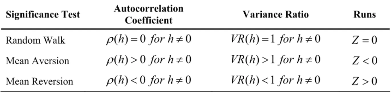
Table 1 summarizes the conclusions of the various test approaches which are applied to test for weak-form market efficiency and return predictability of real estate stock markets.

Table 1: Null and Alternative Hypotheses of Weak-Form Market Efficiency Tests Significance Test Autocorrelation

Coefficient Variance Ratio Runs

Random Walk

U

( )

h

0

for h

z

0

VR h

( ) 1

for h

z

0

Z

0

U

( )

h

!

0

for h

z

0

VR h

( ) 1

!

for h

z

0

Z

0

U

( )

h

0

for h

z

0

VR h

( ) 1

for h

z

0

Z

!

0

3

Empirical Results of Weak-Form Market Efficieny Tests

3.1 Data

Due to its global character, it is necessary to analyze the data set for consistency and comparability to avoid systematic errors. Especially at the index level, it is important to ensure that the indices are constructed according to the same rules and logic and that they equally reflect the development of their respective markets. Thus, we employ the following criteria for the selection of index families for national real estate stocks: (1) long data series should be chosen to minimize the impact of one-time shocks, such as the Asian crisis; (2) the selection criteria for single securities should be approximately equal for all indices; (3) the indices should be representative for the respective real estate stock markets; (4) the use of total return indices should be mandatory (legal requirements on dividends, see REITs); (5) a focus on existing portfolio properties is preferable; (6) indices should be calculated at least daily; and (7) they should be based on listed companies only to avoid appraisal bias or spurious autocorrelation of certain types of investment vehicles.

In comparison to other index providers, the indices of the European Public Real Estate Association (EPRA) and its related institutions in Asia (APREA) and North America (NAREIT) fulfill these requirements.5 Therefore, they are used here for the following 14 countries: Australia (AUS), Belgium (BEL), Canada (CAN), France (FRA), Germany (GER), Hong Kong (HK), Italy (ITA), Japan (JAP), the Netherlands (NL), Singapore (SIN), Sweden (SWD), Switzerland (SWZ), United Kingdom (UK), and the United States (USA).

3.2 Descriptive Statistics

Continuously compounded weekly returns from January 1990 to December 2006 are calculated.6 Descriptive statistics for the annualized weekly returns of the EPRA series are presented in Table 2.

5

For detailed information see EPRA (2006). 6

To avoid day-of-the-week effects we choose Wednesdays’ prices for the calculation of weekly log returns. Furthermore, the period under investigation ends before the breakout of the financial crisis in 2007, since this major global event marks a significant structural break in the data. For the empirical results, it is important to keep in mind that the returns for Canada are only available starting in 1997 and results are therefore not comparable. Log differences of prices are used because, for small changes, they approximately equal the rate of return from continuous compounding.

Table 2: Descriptive Statistics of Annualized Weekly EPRA Index Returns from January 1990 to December 2006 (in Local Currency)

Calculations are based on weekly returns (886 observations) with the exception of Canada where returns are only available for the time period from January 1997 to December 2006 (521 weekly observations). ***, **, and * represent significance at the 1%, 5% and 10% level respectively of the null hypothesis of normal distribution of the Jarque-Bera test statistic. The critical values of the ²-distributed test statistic with two degrees of freedom are 9.21, 5.99 and 4.61 (Jarque and Bera, 1980).

Index Mean Min. Max. Std.dev. Skewness Kurtosis J.-B. AUS 0.151 -3.537 3.022 0.837 -0.048 3.822 25.31*** BEL 0.049 -8.561 4.851 0.950 -0.942 13.614 4,289.88*** CAN 0.171 -5.537 4.912 1.154 0.165 6.160 219.15*** FRA 0.133 -4.750 4.696 0.941 -0.386 6.207 401.65*** GER 0.091 -9.585 7.565 1.542 -0.205 8.022 937.41*** HK 0.119 -10.149 11.290 2.194 -0.287 5.622 265.87*** ITA 0.110 -11.057 11.233 1.645 0.080 8.837 1,258.58*** JAP 0.011 -8.196 11.513 2.346 0.416 4.826 148.74*** NL 0.080 -3.750 3.400 0.782 0.059 4.751 113.70*** SIN 0.051 -10.653 12.962 2.449 0.184 6.917 571.41*** SWD 0.021 -8.698 13.529 1.954 0.644 9.767 1,751.68*** SWZ 0.067 -4.837 5.651 1.038 0.196 6.895 565.75*** UK 0.097 -4.699 9.665 1.203 0.496 8.411 1,117.06*** USA 0.160 -4.647 6.043 1.032 -0.214 7.833 869.18***

As can be seen, Australia, France, and the USA reach the highest average annualized weekly returns. The highest volatility appears in Asia as these countries have both the highest standard deviation as well as the highest range of returns. While the results on skewness are mixed, all series are leptokurtic. Thus, the Jarque-Bera test rejects the null of normality for all return series.

3.3 Results of Autocorrelation Test

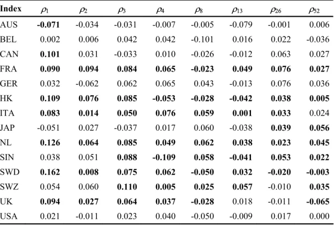
As a first step, the autocorrelations of the weekly returns are calculated. With the exception of Australia, most of the series exhibit significant positive first-order autocorrelation. We can observe significant higher-order autocorrelations, generally of positive sign, at the weekly level. This indicates a general upward trend. These results are in line with the results on stock markets by Poterba and Summers (1988) who report short-term mean aversion processes but mean reversion over the longer run. However, higher-order autocorrelations are insignificant

for Australia and Canada; for Belgium, Germany, and the USA autocorrelation coefficients are insignificant for all lag orders.

Table 3: Autocorrelation of Weekly EPRA Index Returns from January 1990 to December 2006 (in Local Currency)

Calculations are based on weekly returns (886 observations) with the exception of Canada where returns are only available for the time period from January 1997 to December 2006 (521 weekly observations); bold figures indicates significance of the autocorrelation coefficients for lag h at 5% significance level with critical values from the ² distribution with h degrees of freedom.

Index U U U U U U U U AUS -0.071 -0.034 -0.031 -0.007 -0.005 -0.079 -0.001 0.006 BEL 0.002 0.006 0.042 0.042 -0.101 0.016 0.022 -0.036 CAN 0.101 0.031 -0.033 0.010 -0.026 -0.012 0.063 0.027 FRA 0.090 0.094 0.084 0.065 -0.023 0.049 0.076 0.027 GER 0.032 -0.062 0.062 0.065 0.043 -0.013 0.076 0.036 HK 0.109 0.076 0.085 -0.053 -0.028 -0.042 0.038 0.005 ITA 0.083 0.014 0.050 0.076 0.059 0.001 0.033 0.024 JAP -0.051 0.027 -0.037 0.017 0.060 -0.038 0.039 0.056 NL 0.126 0.064 0.085 0.049 0.062 0.038 0.023 0.045 SIN 0.038 0.051 0.088 -0.109 0.058 -0.041 0.053 0.022 SWD 0.162 0.008 0.075 0.062 -0.050 0.032 -0.020 -0.003 SWZ 0.054 0.060 0.110 0.005 0.025 0.057 -0.010 0.035 UK 0.094 0.027 0.064 0.037 -0.028 0.018 -0.011 -0.065 USA 0.021 -0.011 0.023 0.040 -0.050 -0.009 0.017 0.000

Positive autocorrelations are a well-studied phenomenon for stock returns and various possible explanations have been proposed. Lo and MacKinlay (1988) as well as French and Roll (1986) explain autocorrelations in the returns of stock indices by referring to the common risk factor of stocks that comprise the index.7 Thus, systematic risk is driving the autocorrelation. Equally-weighted indices also exhibit stronger evidence for mean aversion

7

than their value-weighted counterparts (Lo and MacKinlay, 1988). These facts also apply to real estate indices, which are primarily composed of small-capitalized members.8

3.4 Results of Variance Ratio Tests

For the VR tests, we use weekly data as a trade-off between short-term persistence and microstructure related dependencies. Presumably, these dependencies are particularly strong for markets with low trading volume and limited liquidity. E.g. for Hong Kong and Singapore results based on daily data may be primarily influenced by the microstructure rather than fundamentals. Monthly intervals, on the other hand, are too large to capture persistence in returns and variance. Thus, daily and monthly data are considered for comparison purpose only. This provides a robustness check to see whether short-horizon price changes behave similar as long-horizon price changes.9 The VRs are computed in intervals of two, four, and eight weeks as well as three and six months (see Table 4).

8

In contrast, Campbell et al. (1997) consider positive autocorrelation to be a result of market microstructure. They argue that non-synchronous trading and bid-ask bounces induce spurious autocorrelation in the returns of stocks and stock indices. However, it seems that by using weekly and monthly data, these issues are mitigated.

9

Table 4: Variance Ratio Estimates VR(q) and Variance Ratio Test Statistics for Weekly Returns of EPRA Indices from January 1990 to December 2006 (in Local Currency)

Calculations are based on weekly returns (886 observations) with the exception of Canada where returns are only avalaible for the time period from January 1997 to December 2006 (521 weekly observations); variance ratio tests of random walk hypothesis for weekly securitized real estate index prices in local currencies; ***, **, * for significance at 99%, 95% and 90% confidence level (rejection of the RWH). One week is taken as a base observation interval; the varaince ratios, VR(q)’s, are reported in bold letters in the main rows. The homoscedasticity- and heteroscedasticity-consistent test results are reported in parentheses ( , ) and brackets [ , ], respectively. The critical values for multiple variance ratio tests and at 1%, 5% and 10% significance level are 3.089, 2.569 and 2.311, respectively, according to Hahn and Hendrickson (1971) and Stoline and Ury (1979).

) q ( Z1 Z1*(q) ) q ( Z2 Z*2(q) Z (q) * 1 Z (q) * 2

Numberq of Base Observations (Lags)

Aggregated to form Variance Ratio Index q = 2 q = 4 q = 8 q = 13 q = 26 SMM form = 5 ^ ` * 1 maxZ 2 ... 26 ^ ` * 2 maxZ 2 ... 26 AUS 0.93 (-2.14)** [-1.80]* 0.84 (-2.53)** [-2.14]** 0.74 (-2.62)*** [-2.29]** 0.70 (-2.31)** [-2.08]** 0.65 (-1.86)* [-1.75]* (-2.62)** [-2.29] BEL 1.00 (0.07) [0.04] 1.03 (0.49) [0.26] 1.10 (1.01) [0.60] 1.03 (0.23) [0.14] 1.11 (0.56) [0.39] (1.01) [0.60] CAN 1.10 (2.40)** [1.74]* 1.16 (1.93)* [1.47] 1.24 (1.83)* [1.44] 1.24 (1.40) [1.12] 1.36 (1.43) [1.19] (2.40)* [1.74] FRA 1.09 (2.73)*** [2.11]** 1.28 (4.41)*** [3.65]*** 1.55 (5.53)*** [4.74]*** 1.65 (4.93)*** [4.24]*** 1.67 (3.49)*** [3.06]*** (5.53)*** [4.74]*** GER 1.03 (1.01) [0.60] 1.02 (0.33) [0.20] 1.12 (1.19) [0.77] 1.24 (1.80)* [1.22] 1.38 (1.99)** [1.43] (1.99) [1.43] HK 1.11 (3.31)*** [2.37]** 1.29 (4.62)*** [3.45]*** 1.41 (4.15)*** [3.19]*** 1.44 (3.31)*** [2.60]*** 1.20 (1.05) [0.85] (4.62)*** [3.45]*** ITA 1.08 (2.52)** [1.91]* 1.17 (2.69)*** [2.08]** 1.33 (3.35)*** [2.65]*** 1.52 (3.92)*** [3.15]*** 1.69 (3.58)*** [2.98]*** (3.91)*** [3.15]*** JAP 0.95 (-1.50) [-1.37] 0.94 (-1.03) [-0.90] 0.91 (-0.92) [-0.81] 0.88 (-0.89) [-0.78] 0.88 (-0.63) [-0.56] (-1.50) [-1.37] NL 1.13 (3.78)*** [3.08]*** 1.30 (4.71)*** [3.96]*** 1.52 (5.24)*** [4.45]*** 1.71 (5.38)*** [4.62]*** 1.90 (4.69)*** [4.17]*** (5.38)*** [4.62]*** SIN 1.04 (1.20) [0.70] 1.16 (2.55)** [1.50] 1.22 (2.17)** [1.33] 1.31 (2.38)** [1.51] 1.26 (1.34) [0.90] (2.55)* [1.51] SWD 1.16 (4.89)*** [2.46]** 1.30 (4.71)*** [2.55]*** 1.47 (4.75)*** [2.89]** 1.55 (4.15)*** [2.71]** 1.88 (4.61)*** [3.04]*** (4.89)*** [3.04]** SWZ 1.06 (1.65)* [1.19] 1.20 (3.13)*** [2.31]** 1.35 (3.51)*** [2.70]*** 1.48 (3.62)*** [2.82]*** 1.65 (3.39)*** [2.66]*** (3.62)*** [2.82]** UK 1.11 (2.87)*** [2.16]** 1.20 (3.25)*** [2.63]*** 1.37 (3.75)*** [3.04]*** 1.43 (3.24)*** [2.65]*** 1.67 (3.50)*** [2.95]*** (3.75)*** [3.04]** USA 1.02 (0.70) [0.44] 1.04 (0.58) [0.39] 1.11 (1.16) [0.82] 1.14 (1.04) [0.76] 1.15 (0.80) [0.63] (1.16) [0.82]

With the exception of Australia and Japan, the returns of all indices exhibit VRs greater than one and suggest that the increase in variance is greater than postulated under the RWH. This confirms the prior results of a mean aversion process because all indices that have a VR of below one at lag two also exhibit negative first-order autocorrelation. Similar results can be reported for those indices with a VR greater than one. The general tendencies for each index remain similar for greater lag lengths. At all lag lengths, Australia and Japan show an under-proportional increase in variance, while the other markets reveal a continuation of the over-proportional increase. The VRs of several countries are significant but all suggest a mean aversion process; with the exception of Australia which has VRs significantly below one. Thus, Australia shows significant signs of a mean reversion process.

Based on the assumption of homoscedasticity, the test statistics for France, Italy, the Netherlands, Sweden, Switzerland, and the UK display, at all lags, significant VRs greater than one and they have a tendency to increase. Contrary to the prediction of mean reversion, this implies that there is persistence in returns for up to half a year. To a lesser extent, this applies also for the other series with a VR greater than one. Australia, however, develops in the opposite direction with decreasing VRs that are consistently below one. Hong Kong and Singapore are the only two series that show an initial increase and a subsequent decrease in the ratios and thus a possible reduction in persistence. Adjusting the tests for heteroscedasticity changes the results because the test statistics are formulated more restrictive. As expected, the VRs are in some cases no longer significant or at a less restrictive level. Nevertheless, the general results about the decision of weak-form efficient or inefficient market remain.

Considering multiple lag lengths simultaneously results in a rejection of the RWH for France, Hong Kong, Italy, the Netherlands, Sweden, Switzerland, and the UK at a high level of significance. The results for Australia, Canada, and Singapore are merely significant at a lower level for the tests under homoscedasticity and therefore show an over proportional increase in variance due to heteroscedasticity. The RWH cannot be rejected by the MVR tests for Belgium, Germany, Japan, and the USA which is in line with the findings according to higher-order autocorrelation.

3.5 Results of Runs Test

Non-autocorrelated financial market returns do not necessarily imply market efficiency (Lucas, 1978; Summers 1986), especially because of the reported skewness and kurtosis in

the returns of Table 2. Moreover, if the return generating process is non-linear, the autocorrelation coefficient is not a reliable measure to detect market (in)efficiency. Therefore, we employ a direct test for market efficiency that does not require the assumption of normality of the underlying distribution. The results of the non-parametric runs test of independence between successive events in time series are presented in Table 5.

Table 5: Results of the Runs Test for Weekly EPRA Index Returns from January 1990 to December 2006 (in Local Currency)

***

, ** and * indicate significance at the 99%, 95% and 90% confidence level; critical values for the runs test at the 1%, 5% and 10% significance level are derived from standard normal distribution.

Runs Index actual Runs N expected [ ] E Runs Probability S Test Statistics AUS 468 434 0.572 2.282** BEL 411 443 0.521 -2.063** CAN 246 257 0.559 -0.898 FRA 409 438 0.556 -1.850* GER 429 443 0.524 -0.839 HK 417 443 0.522 -1.654* ITA 434 442 0.527 -0.485 JAP 472 443 0.502 1.983** NL 396 441 0.541 -2.910*** SIN 402 443 0.508 -2.712*** SWD 413 443 0.504 -1.980** SWZ 438 442 0.526 -0.223 UK 406 442 0.532 -2.321** USA 411 437 0.562 -1.642

The majority of indices show a negative test statistic as can be seen in Table 5. This indicates a mean aversion process because the number of observed runs is below the statistically expected number. For all 14 securitized real estate markets, the results of the different tests are consistent for each market. The results from Table 5 as well as those from the autocorrelation and VR tests suggest a rejection of the RWH for the real estate stock returns of the Netherlands, Sweden, and UK at the 5% significance level and of France and Hong Kong at a 10% level for the runs test. Theses markets show a mean aversion process. In

contrast, there is strong empirical evidence that the Australian market is mean-reverting. Mixed results are obtained for Belgium, Canada, Italy, Japan, Singapore, and Switzerland. While the autocorrelation and the VR tests do not reject the null hypothesis of a random walk for Belgium, Japan, and Singapore, the runs tests suggest that the return generating process does not follow a random walk. The opposite finding applies for Canada, Italy, and Switzerland where at least the autocorrelation or VR tests reject the RWH, but not the runs test. This could be due to the weaknesses in the assumptions related to the return generating process. The RWH is not rejected by any test for Germany and the USA.

The conclusions and results for daily, weekly and monthly data are summarized in Table 6. Persistence in the return series and thus, the rejection of the RWH decreases with lower data frequency.

Table 6: Summary of the Results of the Test Statistics for Daily, Weekly, and Monthly EPRA Index Returns from January 1990 to December 2006 (in Local Currency)

X denotes rejection of the RWH at 5% significance level according to the first-order autocorrelation coefficient, the runs test, the VR tests for one or more q observation intervals with q = 2, 4, 8, 13, and 26 under the assumption of heteroscedasticity, and for multiple VR test for m = 5; O denotes acceptance of the null hypothesis.

Index Autocorrelation

Test Variance Ratio Test

Multiple Variance

Ratio Test Runs Test

Daily Results AUS O O O O BEL X X X X CAN X X X O FRA O X X X GER O O O X HK X X X X ITA O O O X JAP X X X O NL X X X O SIN X X X O SWD X X X O SWZ X X X X UK X X X O USA X X X X Weekly Results AUS X X O X BEL O O O X CAN X O O O FRA X X X O GER O O O O HK X X X O ITA X X X O JAP O O O X NL X X X X SIN O O O X SWD X X X X SWZ O X X O UK X X X X USA O O O O Monthly Results AUS X X O O BEL O O O X CAN O O O O FRA X X X X GER X X O O HK O O O O ITA O X O O JAP O O O O NL X X X X SIN O O O O SWD O X O X SWZ O O O O UK O X O X USA O O O O

3.6 Conditional Variance Ratios

The VR results of Table 4 are only static and reflect average values for the period under investigation. More pertinent insights about efficiency can be achieved by estimating the dynamics implied by the VR. Substituting the empirical variance by conditional volatility from a GARCH(1,1) process allows us to model the VRs dynamically. In doing so, the conditional VR (CVR) is estimated by replacing V ˜ˆ [ ]2 of Equation (3) by the conditional variance:

>

@

> @

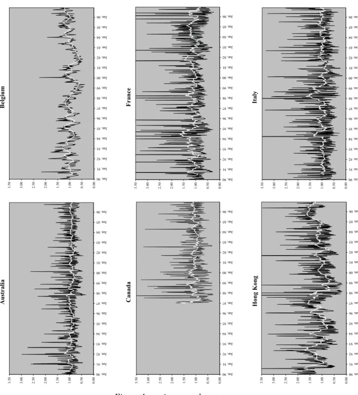
where is the conditional variance of a GARCH(1,1) model assuming a conditional normal distribution, (Engle, 1982; Bollerslev, 1986). To raise the signal to noise ratio of the results from the dynamic analysis of the CVRs, we smooth the CVRs series by calculating moving averages over 26 weeks. From Figure 1 we can see that, in general, the CVRs do not exceed a value of 1.5 and show mean aversion. This is in line with the results from the conventional VRs reported in Table 4. However, the original CVRs fluctuate strongly for the real estate markets of France, Hong Kong, Italy, Japan, the Netherlands, Singapore and the UK.10 In most of the real estate markets, significant increases in the CVRs can be detected during 1998 (Asian crisis) and during 2000/01 when the new economy bubble burst.

t h 2 -1 1 ˆ ˆ ˆ q p t j t j j i h Z

¦

¦

The variability in the CVRs with an observation interval of q = 4 is much higher, with the exception of Australia, Canada, and Japan (see Figure 2). The strongest fluctuations in the CVRs can be observed for the public real estate market of Switzerland.

10

Germany, Sweden, and Switzerland have to be excluded because either estimations do not converge or parameter violations in the GARCH(1,1) equation occur.

Figure 1: Conditional Variance Ratio (CVR) Test (q = 2)

Figure 1 continues on the next page

France 0.00 0.50 1.00 1.50 2.00 2.50 3.00 3.50 Jan. 90 Jan. 91 Jan. 92 Jan. 93 Jan. 94 Jan. 95 Jan. 96 Jan. 97 Jan. 98 Jan. 99 Jan. 00 Jan. 01 Jan. 02 Jan. 03 Jan. 04 Jan. 05 Jan. 06 Belgi um 0. 00 0. 50 1. 00 1. 50 2. 00 2. 50 3. 00 3. 50 Jan. 90 Jan. 91 Jan. 92 Jan. 93 Jan. 94 Jan. 95 Jan. 96 Jan. 97 Jan. 98 Jan. 99 Jan. 00 Jan. 01 Jan. 02 Jan. 03 Jan. 04 Jan. 05 Jan. 06 It aly 0.00 0.50 1.00 1.50 2.00 2.50 3.00 3.50 Jan. 90 Jan. 91 Jan. 92 Jan. 93 Jan. 94 Jan. 95 Jan. 96 Jan. 97 Jan. 98 Jan. 99 Jan. 00 Jan. 01 Jan. 02 Jan. 03 Jan. 04 Jan. 05 Jan. 06 Ho ng K o ng 0.00 0.50 1.00 1.50 2.00 2.50 3.00 3.50 Jan. 90 Jan. 91 Jan. 92 Jan. 93 Jan. 94 Jan. 95 Jan. 96 Jan. 97 Jan. 98 Jan. 99 Jan. 00 Jan. 01 Jan. 02 Jan. 03 Jan. 04 Jan. 05 Jan. 06 Ca na d a 0.00 0.50 1.00 1.50 2.00 2.50 3.00 3.50 Jan. 90 Jan. 91 Jan. 92 Jan. 93 Jan. 94 Jan. 95 Jan. 96 Jan. 97 Jan. 98 Jan. 99 Jan. 00 Jan. 01 Jan. 02 Jan. 03 Jan. 04 Jan. 05 Jan. 06 A u stralia 0.00 0.50 1.00 1.50 2.00 2.50 3.00 3.50 Jan. 90 Jan. 91 Jan. 92 Jan. 93 Jan. 94 Jan. 95 Jan. 96 Jan. 97 Jan. 98 Jan. 99 Jan. 00 Jan. 01 Jan. 02 Jan. 03 Jan. 04 Jan. 05 Jan. 06

Netherlands 0.00 0.50 1.00 1.50 2.00 2.50 3.00 3.50 Jan. 90 Jan. 91 Jan. 92 Jan. 93 Jan. 94 Jan. 95 Jan. 96 Jan. 97 Jan. 98 Jan. 99 Jan. 00 Jan. 01 Jan. 02 Jan. 03 Jan. 04 Jan. 05 Jan. 06 UK 0.00 0.50 1.00 1.50 2.00 2.50 3.00 3.50 Jan. 90 Jan. 91 Jan. 92 Jan. 93 Jan. 94 Jan. 95 Jan. 96 Jan. 97 Jan. 98 Jan. 99 Jan. 00 Jan. 01 Jan. 02 Jan. 03 Jan. 04 Jan. 05 Jan. 06 Ja pa n 0.00 0.50 1.00 1.50 2.00 2.50 3.00 3.50 Jan. 90 Jan. 91 Jan. 92 Jan. 93 Jan. 94 Jan. 95 Jan. 96 Jan. 97 Jan. 98 Jan. 99 Jan. 00 Jan. 01 Jan. 02 Jan. 03 Jan. 04 Jan. 05 Jan. 06 Singapore 0.00 0.50 1.00 1.50 2.00 2.50 3.00 3.50 Jan. 90 Jan. 91 Jan. 92 Jan. 93 Jan. 94 Jan. 95 Jan. 96 Jan. 97 Jan. 98 Jan. 99 Jan. 00 Jan. 01 Jan. 02 Jan. 03 Jan. 04 Jan. 05 Jan. 06 USA 0.00 0.50 1.00 1.50 2.00 2.50 3.00 3.50 Jan. 90 Jan. 91 Jan. 92 Jan. 93 Jan. 94 Jan. 95 Jan. 96 Jan. 97 Jan. 98 Jan. 99 Jan. 00 Jan. 01 Jan. 02 Jan. 03 Jan. 04 Jan. 05 Jan. 06

Conditional variance ratios (black line) are calculated for q = 2 and smoothed by using a moving average of 26 weeks (white line); the conditional variances are estimated by a GARCH(1,1) model according to Equation (10); estimations for international securitized real estate markets of Germany, Sweden, and Switzerland have to be excluded because either estimations do not converge or parameter violations in the GARCH(1,1) equation occur.

Figure 2: Conditional Variance Ratio (CVR) Test (q = 4)

Figure 2 continues on the next page

It aly 0.00 0.50 1.00 1.50 2.00 2.50 3.00 3.50 Jan. 90 Jan. 91 Jan. 92 Jan. 93 Jan. 94 Jan. 95 Jan. 96 Jan. 97 Jan. 98 Jan. 99 Jan. 00 Jan. 01 Jan. 02 Jan. 03 Jan. 04 Jan. 05 Jan. 06 France 0. 00 0. 50 1. 00 1. 50 2. 00 2. 50 3. 00 3. 50 Jan. 90 Jan. 91 Jan. 92 Jan. 93 Jan. 94 Jan. 95 Jan. 96 Jan. 97 Jan. 98 Jan. 99 Jan. 00 Jan. 01 Jan. 02 Jan. 03 Jan. 04 Jan. 05 Jan. 06 Belgi um 0. 00 0. 50 1. 00 1. 50 2. 00 2. 50 3. 00 3. 50 Jan. 90 Jan. 91 Jan. 92 Jan. 93 Jan. 94 Jan. 95 Jan. 96 Jan. 97 Jan. 98 Jan. 99 Jan. 00 Jan. 01 Jan. 02 Jan. 03 Jan. 04 Jan. 05 Jan. 06 Ho ng K o ng 0.00 0.50 1.00 1.50 2.00 2.50 3.00 3.50 Jan. 90 Jan. 91 Jan. 92 Jan. 93 Jan. 94 Jan. 95 Jan. 96 Jan. 97 Jan. 98 Jan. 99 Jan. 00 Jan. 01 Jan. 02 Jan. 03 Jan. 04 Jan. 05 Jan. 06 Ca na d a 0.00 0.50 1.00 1.50 2.00 2.50 3.00 3.50 Jan. 90 Jan. 91 Jan. 92 Jan. 93 Jan. 94 Jan. 95 Jan. 96 Jan. 97 Jan. 98 Jan. 99 Jan. 00 Jan. 01 Jan. 02 Jan. 03 Jan. 04 Jan. 05 Jan. 06 A u stralia 0.00 0.50 1.00 1.50 2.00 2.50 3.00 3.50 Jan. 90 Jan. 91 Jan. 92 Jan. 93 Jan. 94 Jan. 95 Jan. 96 Jan. 97 Jan. 98 Jan. 99 Jan. 00 Jan. 01 Jan. 02 Jan. 03 Jan. 04 Jan. 05 Jan. 06

UK 0.00 0.50 1.00 1.50 2.00 2.50 3.00 3.50 Jan. 90 Jan. 91 Jan. 92 Jan. 93 Jan. 94 Jan. 95 Jan. 96 Jan. 97 Jan. 98 Jan. 99 Jan. 00 Jan. 01 Jan. 02 Jan. 03 Jan. 04 Jan. 05 Jan. 06 Singapore 0.00 0.50 1.00 1.50 2.00 2.50 3.00 3.50 Jan. 90 Jan. 91 Jan. 92 Jan. 93 Jan. 94 Jan. 95 Jan. 96 Jan. 97 Jan. 98 Jan. 99 Jan. 00 Jan. 01 Jan. 02 Jan. 03 Jan. 04 Jan. 05 Jan. 06 USA 0.00 0.50 1.00 1.50 2.00 2.50 3.00 3.50 Jan. 90 Jan. 91 Jan. 92 Jan. 93 Jan. 94 Jan. 95 Jan. 96 Jan. 97 Jan. 98 Jan. 99 Jan. 00 Jan. 01 Jan. 02 Jan. 03 Jan. 04 Jan. 05 Jan. 06 Sw itz erland 0.00 0.50 1.00 1.50 2.00 2.50 3.00 3.50 Jan. 90 Jan. 91 Jan. 92 Jan. 93 Jan. 94 Jan. 95 Jan. 96 Jan. 97 Jan. 98 Jan. 99 Jan. 00 Jan. 01 Jan. 02 Jan. 03 Jan. 04 Jan. 05 Jan. 06 Ja pa n 0.00 0.50 1.00 1.50 2.00 2.50 3.00 3.50 Jan. 90 Jan. 91 Jan. 92 Jan. 93 Jan. 94 Jan. 95 Jan. 96 Jan. 97 Jan. 98 Jan. 99 Jan. 00 Jan. 01 Jan. 02 Jan. 03 Jan. 04 Jan. 05 Jan. 06

Conditional variance ratios (black line) are calculated for q = 4 and smoothed by using a moving average of 26 weeks (white line); the conditional variances are estimated by a GARCH(1,1) model according to Equation (10); estimations for international securitized real estate markets of Germany, the Netherlands, Sweden, and Switzerland have to be excluded because either estimations do not converge or parameter violations in the GARCH(1,1) equation occur.

4

Implications for Trading Strategies

4.1 Moving Average Trend Indicators

Due to potential inefficiencies in most of the global securitized real estate markets, it is possible to derive certain investment strategies and implement them in a corresponding trading system. The rejection of the weak-form EMH, however, does not postulate market inefficiency. Even if the rejection of the RWH as a role model of weak information efficiency is caused by inefficiencies, the question arises whether this inefficiency can be capitalized. Numerous studies reach the conclusion that trading systems that are based on stock market inefficiency cannot be executed profitably when trading costs are accounted for (Fama and Blume, 1966). Thus, Elton et al. (2007) point out that autocorrelation is not necessarily contradictory to the EMH as long as the implementation of a trading strategy is not beneficial due to transaction costs.

Thus, further methods must be introduced to evaluate particular strategies and to provide more direct evidence of market inefficiencies. Technical analysis can therefore serve as a control of or complement to the earlier statistical testing methods.

Moving averages are applied to distinguish between long-term trends and short-term oscillations and act as trend indicators. In practice, the average price is calculated from past trading days. The number of relevant trading days depends on the selected period under investigation. In order to recognize mid- to long-term trends, the 200-days line is used. However, moving averages do not only differ with respect to the length of period (e.g. 200, 30, 10, 5 days), but also with regard to the calculation of the mean. In the simplest form, the arithmetic mean is used.11 As trading strategies are based on daily data, results should be interpreted in reference to the test statistics based on daily data. With daily data, the RWH is rejected in about 70% of the tests (54% for weekly, 32% for monthly data, respectively). To compare the results of the RWH of the previous section, we apply trading strategies based on moving averages for the 14 national real estate market indices as a robustness check. A

11

Models with linearly or exponentially weighted average are also possible. Differences between these approaches are rather small. Thus, the method of the arithmetic mean will be used when calculating averages.

called buying signal occurs if the share quotation breaks through its moving average bottom-up; a selling signal happens when the moving average is breached top-down (see Figure 3).12

Figure 3: Illustration of Buy- and Sell-Indication According to the Moving Average Rule (for the 200-Days Line)

0 200 400 600 800 1.000 1.200 1.400 1.600 04.1 0.199 0 04.1 0.199 1 04.1 0.19 92 04.1 0.19 93 04.1 0.19 94 04.1 0.19 95 04.1 0.199 6 04.1 0.199 7 04.1 0.199 8 04.1 0.199 9 04.1 0.20 00 04.1 0.20 01 04.1 0.20 02 04.1 0.20 03 04.1 0.200 4 04.1 0.200 5 04.1 0.200 6

EPRA-Index Hong Kong Moving Average

Sell-Indication

Buy-Indication Buy-Indication

Sell-Indication

In addition to the 200-day window, moving-averages for 5, 10, and 30 days are calculated. This is advantageous for indices that are more volatile. However, it has to be considered that the advantage of more frequent portfolio turnovers may be reduced by higher transaction costs.

A trading signal occurs directly at the breakthrough of the 200-days line on closing call under the assumption that a trade on closing call is possible and will be the opening call of the next day. Further, we assume that indices are either directly projected by derivatives (e.g. index derivatives) and can be purchased or are individually synthetically reproducible and therefore possess the same characteristics as the index itself. Next, we suppose that the investment volume of the strategy is large enough. Therefore, the same accruing transaction costs should

12

As there is no theoretical answer which two moving averages to combine when using them as trading signals, only long-term trend movements are considered in this analysis.

apply, which are considered to be 0.1% per transaction.13 As a result, the same conditions should be valid for the synthetic reproduction of the portfolio as for a direct investment in the index. Hence, the investment volume in single shares should also be adequate to exploit all scale effects. Further, we assume liquid markets with no significant market impact by individual traders. When selling a position due to trend indication, a conservative investment based on current call money rates is supposed. We do not use average rates over the relevant time horizon because the timeframe of about 17 years can catch more than one economic or interest cycle. Thus, average values could lead to significant distortions.14

The sample period ranges from October 5, 1990 to December 31, 2006 which is identical to the sample for the tests of the RWH. The time period from January 1, 1990, to October 4, 1990, is needed to compute the moving average based on the 200-days line. Therefore, the moving averages of October 4, 1990, serve as starting points and decision criteria for the positioning of the money and stock market. A statistical advantage of this strategy is that it relies on out-of-sample observations.

The chart-technical model is compared with the buy-and-hold-strategy. The technical model is advantageous when considering transaction costs; it generates higher returns than a simple buy-and-hold-strategy. Even before interpreting the empirical results, it has to be mentioned that a strategy derived from moving averages has lower risk compared to buy-and-hold-strategy in the sense of volatility. This is because in weak market phases, the positions are shifted into the money market. Thus, the investor is not present in negative market phases and the risk of her investment is minimized.

Table 7 shows the average annual returns of the two strategies. In a first step, a market without transaction costs is assumed, whereas in a second step, the analysis is applied to a market environment with transaction costs. Since frequent transactions reduce the total profits, especially in markets with a relatively low volatility in returns, a long-term-oriented strategy based on the 200-days moving average should prove advantageous compared to one based on shorter averages. Yet, in highly volatile markets like those of Hong Kong and Singapore even shorter moving averages may be reasonable.

13

The same approach for transaction costs of a floor trader is also chosen by Fama and Blume (1966). Due to technical progress with the handling of transactions, the actual costs should be even lower today.

14

Applying call money rates instead of short positions is motivated by the fact that the latter alternative is only available with securitized real estate products.

Table 7: Returns p.a. of Trading Strategies Based on Moving Averages (for Canada shortened time period)

Moving Averages

without / with Transaction Costs Index # of Test Statistics (out of 4; daily) rejecting RWH Buy-&-Hold

Strategy _{5 Days 10 Days 30 Days 200 Days}

AUS 0 15.80% 9.92% / 2.43% 8.65% / 3.65% 8.79% / 6.03% 11.55% / 10.63% BEL 4 6.45% -3.66% / -10.82% -0.64% / -5.63% 4.24% / 1.56% 8.52% / 8.04% CAN 3 12.53% 18.20% / 10.78% 36.93% / 11.20% 11.52% / 8.88% 13.03% / 12.34% FRA 3 15.83% 13.40% / 6.01% 14.57% / 9.57% 18.59% / 16.17% 17.63% / 17.10% GER 1 7.70% 10.01% / 3.33% 9.76% / 5.37% 9.21% / 7.00% 8.87% / 8.22% HK 4 12.45% 36.98% / 29.05% 31.19% / 26.29% 24.66% / 22.10% 17.57% / 16.89% ITA 1 11.56% 11.77% / 4.32% 11.52% / 6.69% 12.40% / 9.74% 15.80% / 15.11% JAP 3 6.14% 9.89% / 2.59% 4.06% / -0.67% 12.05% / 9.71% 4.23% / 3.19% NL 3 9.90% 17.18% / 10.80% 16.10% / 12.10% 15.39% / 13.30% 12.84% / 12.33% SIN 3 7.66% 28.46% / 20.61% 20.56% / 15.68% 22.30% / 19.85% 13.90% / 12.92% SWD 3 2.72% 19.66% / 12.38% 21.04% / 16.22% 17.05% / 16.48% 21.89% / 16.67% SWZ 4 8.73% -14.44% / -21.56% -6.96% / -12.21% -2.96% / -6.19% 8.28% / 7.49% UK 3 13.12% 18.07% / 11.03% 15.90% / 11.17% 18.85% / 16.62% 18.51% / 18.21% USA 4 20.25% 22.61% / 15.32% 19.27% / 14.58% 18.30% / 15.84% 18.10% / 17.38%

The third object of investigation is to analyze to what extend the test results of the RWH are confirmed by the technical analysis method. In the first step, where transaction costs are neglected, the trading strategy is dominated by the simple buy-and-hold-strategy only in cases of Australia and Switzerland. While the RWH is accepted for Australia for all testing

procedures, it is rejected for Switzerland (see Table 6). All other remaining indices show at least one moving average strategy that can generate a more favorable return.

Six of the analyzed real estate indices show higher returns for all analyses based on moving averages than for a continuous market investment. While the additional returns are less than 4% p.a. for Belgium, Germany, Italy and the USA, differences in returns of up to 24% p.a. can be observed for Hong Kong, Singapore and Sweden. As expected, shorter moving averages prove to be relatively beneficial, with differences in returns of up to 20% for the highly volatile markets of Hong Kong and Singapore. By contrast, the indices for Germany, Italy, the Netherlands, Sweden, and the UK exhibit relatively constant average returns, independently of the selection of the moving average.

Although the assumptions of the RWH appear to hold for the index of securitized real estate investments for countries such as Germany, excess market returns can be generated by employing the method of moving averages. Potential reasons for this result could be statistical inaccuracies and non-linear return generation processes. A further reason could be that excess market returns cannot be realized because of transaction costs and trading barriers.

Considering transaction costs in the amount of 0.1% of the value of the portfolio at the time of the transaction, the buy-and-hold-strategy dominates all trading strategies based on moving averages for Australia, Canada, Switzerland, and the USA. Thus, for the last three markets, the results of the chart-technical analysis correspond to those of VRs and runs tests. Also, for Belgium, Germany, Italy and Japan, only the moving average strategy including long-term trend indicators generates a higher return. In contrast, the number of transactions of short-term indicators is ten times as high as the number of long-short-term indicators. The transaction costs therefore absorb a substantial fraction of the additional returns. While there are substantial differences in short-term returns (up to approx. 8%), in the long-term, returns differ by more than 1% only for Sweden. The tendency that longer moving averages provide a trading signal that leads to a beneficial strategy with transaction costs is confirmed for France and the UK. However, consistently higher returns are obtained for Hong Kong, the Netherlands, Singapore, and Sweden.

In sum, the results confirm that the rejection of the RWH is also reflected in an excess return generating trading strategy compared to buy-and-hold. The only exception is the U.S. real estate market with the highest market capitalization and trading volume.

4.2 Risk-Adjusted Performance of Trading Strategy

Regarding returns, the results indicate that applying the method of moving averages as a trading signal is an advantageous strategy. At the same time, the analyzed trading model is associated with a significantly reduced risk. The variances of the different trading strategies turn out to be significantly different at a 1% level compared to the buy-and-hold-strategy according to variance test. The variance resulting from the buy-and-hold-strategy is higher for all time series.

To control for the risk-adjusted performance of the trading strategies we statistically compare the Sharpe ratios between the strategy and buy-and-hold portfolios by using the procedure of Gibbson et al. (1989). The test statistic W (W follows a Wishart-distribution) is calculated as 2 2 1 1 1 i j SR W SR § ¨ ¸ ¨ ¸ © ¹ · , with , (11) po states H i j SR tSR

where the null hy thesis ₀:SR_i SR_j. Via transformation, a central-F-distributed

test statistic with N and (T N 1) degrees of freedom can be derived from the test statistic

W, ,( 1) ( 1) ( 2) N T N T T N W F N T , (12) is applied. For Singapore significant results are mainly observed for short-term indicators.

with N indicating the number of securities and T the number of observations.

Following this methodology, the test results confirm the superiority of the trading strategy (see Table 8). This applies in particular to the moving averages over 30 and 200 days for the French, Hong Kong, Dutch, Swedish, and UK indices. Considering the Italian market, this methodology is only advantageous when the 200-days moving average

Table 8: Sharpe Ratios’ Test Statistics for Portfolio Alternatives

On a 10% level of significance, greater Sharpe-Ratios – in comparison to the buy-and-hold portfolio – are marked with an X; a tag with an O represents a result without any significance or rather that the strategy is not advantageous compared with the buy-and-hold-strategy.

Index 5 Days MA 10 Days MA 30 Days MA 200 Days MA

AUS O O O O BEL O O O O CAN O O O O FRA O O X X GER O O O O HK X X X X ITA O O O X JAP O O O O NL X X X X SIN X X X O SWD O X X X SWZ O O O O UK O O X X USA O O O O

To sum up, applying moving averages over the whole period leads to higher returns and lower risk in comparison to using a buy-and-hold-strategy.

5 Conclusion

The efficient market hypothesis (EMH) deals with the question whether stock prices fully reflect all information available at a specific point in time. Weak-form tests of the EMH model focus on the information set of historical prices or return series. This study examines the behavior of weekly securitized real estate returns for 14 countries over the period of January 1990 to December 2006. The tests utilize single (VR) and multiple variance ratio (MVR) tests because they possess greater power and a lower sensitivity against type-II error than conventional tests, such as autocorrelation and unit root tests, even if the time series are not normally distributed. Variance ratio tests also allow the random walk hypothesis (RWH) to be tested jointly for all observation intervals. Since the rejection of the RWH does not necessarily imply inefficiency in a market, a non-parametric runs test for market efficiency is

also conducted. Additionally, the practical relevance of rejecting the RWH is tested by implementing trading strategies based on moving averages.

The results show that the return generating process of real estate stock markets significantly differs from the theoretical model of the RWH. According to the variance ratio and runs tests public real estate markets are mostly inefficient. Furthermore, these results are confirmed by the risk-adjusted performance of the moving average strategy which shows lower risk and higher returns compared to the buy-and-hold-strategy.

In general, we can conclude that investors are likely to earn excess returns by using past information in most of the public real estate markets.

References

Abraham, A., F.J. Fazal, and S.A. Alsakran (2002): “Testing the Random Walk Behavior and

Efficiency of the Gulf Stock Markets”, The Financial Review 37(3), 469-480.

Agbeyegbe, T.D. (1994): “Some Stylised Facts about the Jamaica Stock Market”, Social and

Economic Studies 43(4), 143-156.

Barnes, P. (1986): “Thin Trading and Stock Market Efficiency: The Case of the Kuala

Lumpur Stock Exchange”, Journal of Business Finance & Accounting 13(4), 609-617.

Bollerslev, T. (1986): “Generalized Autoregressive Conditional Heteroscedasticity”, Journal

of Econometrics 31(3), 307–327.

Box, G., and D. Pierce (1970): “Distribution of Residual Autocorrelations in Autoregressive

Integrated Moving Average Time Series Models”, Journal of the American Statistical

Association 65(332), 1509-1526.

Butler, K.C., and S.J. Malaikah (1992): “Efficiency and Inefficiency in Thinly Traded Stock

Markets: Kuwait and Saudi Arabia”, Journal of Banking and Finance 16(1), 197-210.

Campbell, J.Y., A.W. Lo, and A.C. MacKinlay (1997): The Econometrics of Financial

Markets, Princeton: Princeton University Press.

Chang, K.-P., and K.-S. Ting (2000): “A Variance Ratio Test of the Random Walk

Hypothesis for Taiwan’s Stock Market”, Applied Financial Economics 10(5), 525-532.

Chaudhuri, K., and Y. Wu (2003): “Random Walk versus Breaking Trend in Stock Prices:

Evidence from Emerging Markets”, Journal of Banking and Finance 27(4), 575-595.

Chow, K.V., and K.C. Denning (1993): “A Simple Multiple Variance Ratio Test”, Journal of

Econometrics 58(3), 385-401.

Dickey, D.A., and W.A. Fuller (1979): “Distribution of the Estimators for Autoregressive

Time-Series with a Unit Root”, Journal of the American Statistical Association 74(366),