Article
Model-Free Stochastic Collocation for an
Arbitrage-Free Implied Volatility, Part II
Fabien Le Floc’h1,* and Cornelis W. Oosterlee1,2
1 Delft Institute of Applied Mathematics, TU Delft, 2628 XE Delft, The Netherlands
2 CWI-Centrum Wiskunde & Informatica, 1098 XE Amsterdam, The Netherlands; [email protected] * Correspondence: [email protected]
Received: 22 January 2019; Accepted: 20 February 2019; Published: 6 March 2019
Abstract: This paper explores the stochastic collocation technique, applied on a monotonic spline, as an arbitrage-free and model-free interpolation of implied volatilities. We explore various spline formulations, including B-spline representations. We explain how to calibrate the different representations against market option prices, detail how to smooth out the market quotes, and choose a proper initial guess. The technique is then applied to concrete market options and the stability of the different approaches is analyzed. Finally, we consider a challenging example where convex spline interpolations lead to oscillations in the implied volatility and compare the spline collocation results with those obtained through arbitrage-free interpolation technique of Andreasen and Huge.
Keywords:stochastic collocation; implied volatility; quantitative finance; arbitrage-free; risk neutral density; B-spline
1. Introduction
Financial markets provide option prices for a discrete set of strike prices and maturity dates. In order to price over-the-counter vanilla options with different strikes, or to hedge complex derivatives with vanilla options, it is useful to have a continuous arbitrage-free representation of the option prices, or equivalently of their implied volatilities. For example, the variance swap replication of Carr and Madan consists in integrating a specific function over a continuum of vanilla put and call option prices (Carr and Madan 2001;Carr and Lee 2009). More generally,Breeden and Litzenberger(1978) have shown that any path-independent claim can be valued by integrating over the probability density implied by market option prices. An arbitrage-free representation is also particularly important for the Dupire local volatility model (Dupire 1994), where arbitrage will translate to a negative local variance. In this paper, we describe a new technique to interpolate the market option prices in an arbitrage-free manner.
A rudimentary, but popular, representation is to interpolate market implied volatilities with a cubic spline across option strikes. Unfortunately, this may not be arbitrage-free as it does not preserve the convexity of option prices in general. A typical convex interpolation of the call option prices by quadratic splines or rational splines is also not satisfactory in general since it may generate unrealistic oscillations in the corresponding implied volatilities, as evidenced in (Jäckel 2014). Kahalé(2004) designs an arbitrage-free interpolation of the call prices, which however requires convex input quotes, employs two embedded non-linear minimizations, and it is not proven that the algorithm for the interpolation function of classC2converges. In reality, it is often not desirable to strictly interpolate option prices as those fluctuate within a bid-ask spread. Interpolation will lead to a noisy estimate of the probability density (which corresponds to the second derivative of the undiscounted call option price). More recently,Andreasen and Huge(2011) have proposed to calibrate the discrete piecewise constant local volatility corresponding to a single-step finite difference discretization of the forward
Dupire equation. In their representation of the local volatility, the authors use as many constants as the number of market option strikes for an optimal fit. It is thus sometimes considered to be “non-parametric”. Their technique works well but often yields a noisy probability density estimate, as the prices are typically over-fitted. Furthermore the output of their technique is a discrete set of option prices, which, while relatively dense, must still be interpolated carefully to obtain the price of options whose strike falls in between nodes.
This paper considers another approach, based on the stochastic collocation technique of
Grzelak and Oosterlee (2017). Instead of collocating on a polynomial as in Le Floc’h and Oosterlee (2019), we explore various ways to use a monotonic spline, including B-spline parametrizations. This allows for a richer representation, with as many parameters as there are market option strikes. A direct consequence is the ability to capture more complex implied probability distributions, such as multi-modal distributions. We pay attention to avoid over-fitting by adding some appropriate regularization. This is reminiscent of the penalized B-spline technique for volatility modelling ofCorlay(2016), where a B-spline parameterization of the Radon–Nikodym derivative of the underlying’s risk-neutral probability density with respect to a roughly calibrated base model is used. Concretely, Corlay’s method translates to an explicit probability density representation where the probability density is a spline multiplied by a base probability density function, such as the lognormal or normal probability density function. Corlay’s technique however limits the implied volatility shapes allowed, and often requires the use of a more elaborate base probability density function, such as the one stemming from the SVI1parameterization ofGatheral(2004), to properly fit the market in practice. We will see that the stochastic collocation on a spline is more flexible and can fit the market very well when collocating to a simple Gaussian variable.
The outline of the paper is as follows. Section2presents how to apply the stochastic collocation on a monotonic cubic spline, while still preserving the first moment exactly. The collocation on an exponential spline is explored in Section3, which results in analytical formulas not only for the price of vanilla options but also for the price of variance swaps. Section4considers B-spline representations which take into account the monotonicity and the martingale constraints explicitly. Section5details the calibration towards market option prices of each kind of representation. Section6explains how to filter the market quotes so that the spline collocation technique can be applied directly. The filtering may be used independently of the B-spline collocation. Finally, Section7explores the stability of the calibration on concrete market data, for the different parametrizations considered. We compare the quality of fit and the implied probability density with the Andreasen–Huge technique, regularized. In Section8, we look at a challenging example ofJäckel(2014), where interpolation splines applied to call prices lead to oscillations in the interpolation.
2. Spline Collocation
Collocation methods are commonly used to solve ordinary or partial differential equations (LeVeque 2007). The underlying principle is to solve the equations in a specific finite dimensional space of solutions, such as polynomials up to a certain degree. In contrast, the stochastic collocation method (Mathelin and Hussaini 2003) consists in mapping a physical random variableYto a pointX in an artificial stochastic space. Collocation pointsxiare used to approximate the function mappingX
toY,FX−1◦FY, typically by a polynomial, whereFX,FYare respectively the cumulative distribution
functions (CDF) ofXandY. Thus, only a small number of inversions ofY(and evaluations ofFY) are
used. This allows the problem to be solved in the “cheaper” artificial space.
1 SVI stands for Stochastic Volatility Inspired. The SVI model consists in five parameters which define the scaled sum of a
In the context of option price interpolation, the stochastic collocation allows us to interpolate the market CDF in a better set of coordinates. In particular, we followGrzelak and Oosterlee(2017) and use a Gaussian distribution forX.
In (Grzelak and Oosterlee 2017), the stochastic collocation is applied to the survival distribution functionGY, where GY(y) = 1−FY(y)withFYbeing the cumulative density function of the asset
price process. When the survival density function is known for a range of strikes, their method can be summarized by the following steps:
1. Given a set of collocation strikesyi,i=0, ...,N, compute the survival densitypiat those points: pi =GY(yi).
2. Project on the Gaussian distribution by transforming thepiusing the inverse cumulative normal
distributionΦ−1resulting inxi=Φ−1(1−pi).
3. Interpolate(xi,yi)with a monotonic and derivable functiongonR.Grzelak and Oosterlee(2017)
use a Lagrange polynomial forgbut the technique can be applied to any derivable and monotonic function. Further on, we will consider a monotonic spline.
4. Price by integrating the density with the integration variablex = Φ−1(1−GY(y)), using the
approximationgto map the coordinatesxto the strikesy.
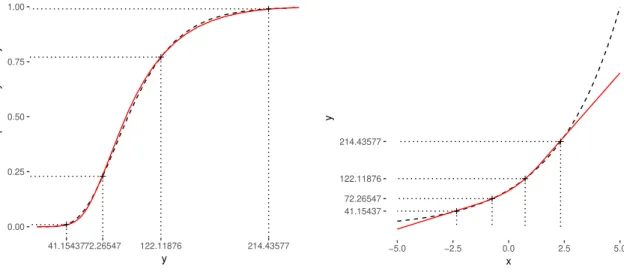
In order to illustrate the mapping involved in the stochastic collocation technique, we consider four options with strikesy0 = 40,y1 = 70, y2 = 120,y3 = 215 and maturity time T = 2 in the Black–Scholes model with constant volatility σ = 20% and forward price to maturity F = 100. Figure1a details the mapping from the four market strikesyito the cumulative probability densitypi
(step 1) and Figure1b shows the mapping from the coordinatexitoyi(step 2). The initial goal of step
3 is to find a smooth function that approximates the theoretical mapping in the coordinates fromxtoy well. The mapping function only needs to be monotonic, and to conserve the first moment, in order for the collocation method to be arbitrage-free. The figures show the mapping with the Black–Scholes model, which constitutes the reference, and with the B-spline collocation presented in this paper, based on the four options. The cumulative density for the B-spline collocation is obtained after computing the optimal collocation B-spline in thex,ycoordinates, based on the four points(xi,yi)i=0,...,3.
0.00 0.25 0.50 0.75 1.00 41.1543772.26547 122.11876 214.43577 y cum ulativ e probability density
mapping B−spline collocation Black−Scholes
(a)Cumulative probability density from strike pricesyi
41.15437 72.26547 122.11876 214.43577 −5.0 −2.5 0.0 2.5 5.0 x y
mapping B−spline collocation Black−Scholes
(b)xifromyi
Figure 1.Mapping in the stochastic collocation technique for the Black–Scholes model with volatility
In reality, we are really interested in minimizing the error in terms of option prices (or equivalently implied volatilities). The discrete set of reference option prices either come directly from the financial markets, or from a prior model. This is where step 4 also becomes critical.
Let us now detail step 4. The undiscounted price of an option with strike priceKis obtained by integrating over the probability densityBreeden and Litzenberger(1978):
C(K) = Z +∞
0 max(y−K, 0)f(y)dy,
where f is the probability density implied by the options prices. We then perform the change of variablex=Φ−1(1−G Y(y))to obtain C(K) = Z Φ−1(1) Φ−1(0) max GY−1(1−Φ(x))−K, 0φ(x)dx. Asg(x)≈GY−1(1−Φ(x)), we have C(K)≈ Z ∞ −∞max(g(x)−K, 0)φ(x)dx = Z ∞ xK (g(x)−K)φ(x)dx, (1)
whereφ(x)is the Gaussian density function and
xK=g−1(K). (2)
The change of variables is valid when the survival density is continuous and its derivative is integrable. In particular, it is not necessary for the derivative to be continuous.
When g is a piecewise cubic polynomial defined on the knots (xi,yi)i=0,...,N, the call option
price can be obtained analytically. Let g(x) = gi(x) = ai+bi(x−xi) +ci(x−xi)2+di(x−xi)3
for x ∈ [xi,xi+1], and k the index such that yk ≤ K < yk+1, assuming that 0 ≤ i < N exists, Equation (1) becomes C(K) =I(x˜−1,x0) +I(x˜N,∞)−KΦ(−x˜k) + N−1
∑
i=k h ai−(bi+di(x˜2i +3))xi+ci(xi2+1) i (Φ(−x˜i)−Φ(−x˜i+1)) + N−1∑
i=k h bi+ci(x˜i−2xi) +di(3x2i −3 ˜xixi+x˜2i +2) i φ(x˜i) − N−1∑
i=k h bi+ci(x˜i+1−2xi) +di(3x2i −3xix˜i+1+x˜2i+1+2) i φ(x˜i+1), (3)with ˜xk =g−1(K), ˜x−1=x0and ˜xi =xifori>k. The integralIcorresponding to the left and right
extrapolations is defined by
I(a,b) = Z b
a g(x)φ(x)dx.
In the case of a linear extrapolation with slopesand starting at the point(x,y), we have IL(a,b) = (y−sx)(Φ(b)−Φ(a))−s(φ(b)−φ(a)).
with the abuse of notationΦ(∞) = 1,Φ(−∞) = 0 andφ(∞) = φ(−∞) = 0. We uses = sL, and x = x0,y = y0 for the left wing extrapolation, and s = sR, and x = xN,y = yN for the right
When K < y0 and in the case of a linear extrapolation, Equation (3) is still valid, but with ˜ x−1= K−y0 sL +x0. WhenK>yN,CK=IR(x˜N,∞)with ˜xN= K−yN sR +xN.
The cut-off point ˜xk = g−k1(K) can be found analytically through Cardano’s formula
(Nonweiler 1968).
The first moment is given by
M1(g) =I(−∞,x0) +I(xN,∞) + N−1
∑
i=0 h ai−(bi+di(x2i +3))xi+ci(x2i +1) i (Φ(xi+1)−Φ(xi)) + N−1∑
i=0 h bi−cixi+di(xi2+2) i φ(xi) (4) − N−1∑
i=0 h bi+ci(xi+1−2xi) +di(3x2i −3xixi+1+x2i+1+2) i φ(xi+1).In practice, the preservation of the martingale property (and the put-call parity relation) imposes M1=FwhereFis the market forward price to maturityT.
The put option price is calculated through the put-call parity relation, namely
C(K)−P(K) =F−K, (5)
whereP(K)is the undiscounted price today of a put option of maturityT, andFis the forward price to maturity.
When put option prices are very small, and assuming that the first moment equals exactly the forward price, it is preferable to use a more direct approach. Equation (5) does not allow to compute prices below machine epsilon. Using the same change of variables as for the call option (Equation (1)), we have for a put option with strikeK:
P(K) = Z +∞ 0 max(K−y, 0)f(y)dy = Z xK −∞(g(x)−K)φ(x)dx. This leads to P(K) =KΦ(x˜k)−I(−∞, ˜x−1)−I(x˜N,xN) + k−1
∑
i=0 h ai−(bi+di(x2i +3))xi+ci(x2i +1) i (Φ(x˜i+1)−Φ(x˜i)) + k−1∑
i=0 h bi+ci(x˜i−2xi) +di(3x2i −3xix˜i+x˜2i +2) i φ(x˜i) (6) − k−1∑
i=0 h bi+ci(x˜i+1−2xi) +di(3x2i −3xix˜i+1+x˜2i+1+2) i φ(x˜i+1),with ˜xk=g−1(K), ˜x−1=x0and ˜xi=xifor 0≤i<k.
3. Exponential Spline Collocation 3.1. Vanilla Options
Instead of interpolating on the strikes (the points(xi,yi)i=0,...,N), we will interpolate the log strikes
positive and that the probability of the asset being negative equals zero. The undiscounted call price of an option with strikeKis then
C(K) = Z ∞
−∞max(e
g(x)−K, 0)
φ(x)dx, (7) wheregis a monotonic piecewise polynomial function interpolating(xi, lnyi)i=0,...,N. We cannot obtain
a closed-form formula for a generalgfunction, if we assume thatgis a quadratic spline. Let(x¯j)j=0,...,M
be the spline knots, andg(x) =aj+bj(x−x¯j) +cj(x−x¯j)2on[x¯j, ¯xj+1], withkthe index such that ¯ yk≤K<y¯k+1, we have then C(K) =I(x˜−1, ¯x0) +I(x˜M,∞) +KΦ(−x˜k) + M−1
∑
j=k eaj−bjx¯j+cjx¯2j+12m2jΦ x¯j+1 p 1−2cj−mj−Φ x˜jp1−2cj−mj p 1−2cj , withmj = bj−2cjx¯j √ 1−2cj and defining ˜xk =g −1(lnK), ˜xi =x¯ifori>k. When 1−2cj <0, we can use the
imaginary error function erfi as we have fora,b∈R,
−iΦ(ib p 2cj−1)−Φ(iap2cj−1) p 2cj−1 = erfi b q2c j−1 2 −erfi a q2c j−1 2 2p 2cj−1 .
For a linear extrapolation with slope s and passing by the point (x,y), corresponding to g(u) =s(u−x) +y, we find I(a,b) = Z b a e s(u−x)+y φ(u)du =ey−sx+12s2(Φ(b−s)−Φ(a−s)) , (8) with some abuse of notationΦ(−∞) =0, Φ(∞) =1. The left wing extrapolation corresponds to
x = x¯0andy = y¯0, withs = sL a free parameter and the right wing extrapolation corresponds to
x = x¯M,y = y¯M withs = sR. In order to keep the continuity of the derivative at the boundaries,
we choosesR=g0(xN)andsL=g0(x0). The first moment is given by
M1= Z ∞ −∞e g(x) φ(x)dx =I(−∞, ¯x0) +I(x¯M,∞) + M−1
∑
j=0 eaj−bjx¯j+cjx¯2j+12m2jΦ x¯j+1 p 1−2cj−mj −Φ x¯jp1−2cj−mj p 1−2cj (9) =I(−∞, ¯x0) +I(x¯M,∞) + M−1∑
j=0 eaj+ b2j−2bjxj¯+2cjx¯2j 2(1−2cj) Φ x¯j+1 p 1−2cj−mj−Φ x¯jp1−2cj−mj p 1−2cj . 3.2. Variance SwapVariance swaps contracts allow a buyer to receive the future realized variance of the price changes until a specific maturity date against a fixed strike price, paid at maturity. Conventionally, these price changes are daily log returns of a specific stock, equity index, or exchange rate based upon the most commonly used closing price (or exchange rate reset price). Variance swaps became particularly
popular after Demeterfi et al. showed that a single contract could be statically replicated by a portfolio of vanilla options (Demeterfi et al. 1999). In the absence of jumps2and assuming the observations to be continuous, the problem of pricing a variance swap can be reduced to the pricing of a log-contract. The price Vof a variance swap, by continuous replication, has a particularly simple closed-form expression with the exponential spline parametrization. For a newly issued variance swap with zero strike, and a transition probability density f fromt = 0 tot = T, followingCarr and Lee(2009), we have V(0,T) =−2 T Z ∞ 0 ln y F(0,T) f(y)dy (10) =−2 T Z ∞ −∞(g(x)−lnF(0,T))φ(x)dx.
In Equation (10), ˜g = g−F(0,T)is a piecewise quadratic spline. The value of the integral corresponds to the first moment of the collocation variable with the spline ˜g, which is given explicitly by Equation (4). The standard replication formula fromCarr and Madan(2001) implies to choose an integration cut-off and to use of a numerical quadrature, typically an adaptive Gauss–Lobatto quadrature. This is not necessary with the exponential spline collocation approach. The price of the variance swap can be adjusted by changing the slope of the linear extrapolation. This allows for a fast joint calibration of the collocating B-spline to market option prices and variance swaps. The market variance swap prices give some additional information on the tail of the distribution, not covered by vanilla options.
4. B-Spline Collocation
We recall that the goal of the stochastic collocation is to find a smooth monotonic function to represent the functiong mapping the abscissas(xi)i=0,...,N to the ordinates (the strikes)(yi)i=0,...,N
(see Figure1b), by minimizing the error in option prices in a least-squares sense. From the previous sections, we now know how to price vanilla options by collocating on a spline, which passes through the specific points(xi,yi)i=0,...N. We can then choose to optimize either the abscissas or the ordinates
of those points in order to minimize the least squares error in option prices, on the condition that we use a monotonicity preserving spline and make sure to conserve the first moment in the optimization.
Instead of using an exact interpolation function on a set of points, and optimizing this interpolation through the choice of points, we can rely on a B-spline representation and optimize directly the B-spline coefficients. The method will work both on the direct strikes, or on the log strikes. We consider a quadratic B-spline representation, that is, B-splines of orderk=3. The B-spline representation ofgon
N+1+kknots reads (De Boor 1978)
g(x) = N
∑
i=0αiBi,3(x). (11)
We choose the nearly optimal knots ti+3 = xi+1+2xi+2 for i = 0, ...,N−3 according to (De Boor 1978, p. 193) with the boundary knotst0 = t1 = t2 = x0andtN+1 = tN+2 = tN+3 = xN.
This choice of knots ensures thatgisC1on[x0,xN].
Because the derivative of the equivalent piecewise polynomial representation is linear between two distinct knots,gwill be monotonically increasing on an interval[ti−1,ti]if and only if the derivative
at the endpoints is positive. Thus,gwill be monotonically increasing on the interval[x0,xN]if and
only ifαi−αi−1>0 fori=1, ...,Nin Equation (11).
It is then particularly simple to impose the monotonicity constraints when we optimize the coefficientsαiduring the calibration to market quotes. Furthermore, a least-squares fit ofgdirectly to
some input(xi,yi)i=0,...,Nreduces to a simple quadratic programming problem:
˜ α=arg min α∈RN+1 1 2α TQ α+qTα (12)
subject toαi−αi−1 > 0 for i = 1, ...,N, with Q = PTP, q = −PTy and Pthe matrix defined by Pi,j=Bi,3(yj). In particular,Pis a banded matrix (De Boor 1978).
The quadratic programming problem is fast to solve using a standard optimization library such as CVXOPT (Andersen et al. 2013), OSQP (Stellato et al. 2017), or quadprog (Turlach and Weingessel 2007), when compared to the total time taken to calibrate the spline. This will allow starting the optimization from a reasonable initial guess.
In order to price an option or to evaluate the first moment, we simply transform the B-spline representation to a piecewise quadratic polynomial (De Boor 1978, p. 117–19) and rely on Sections 2and 3in this paper, for respectively a direct B-spline collocation, and an exponential B-spline collocation.
In the case of the direct B-spline collocation, the first moment is a linear combination of the B-spline coefficients. Indeed, the first moment is a linear combination of the piecewise polynomial coefficients in Equation (4) and the piecewise polynomial coefficients themselves are a linear combination of the B-spline coefficients: aj= tj+2−tj+1 tj+3−tj+1 αj+1−αj+αj, (13) bj=2 αj+1−αj tj+3−tj+1 , (14) cj= 1 tj+3−tj+2 αj+2−αj+1 tj+4−tj+2 + αj−αj+1 tj+3−tj+1 ! . (15)
We can thus add the martingale constraint directly to the quadratic programming problem as an additional equality constraint.
5. Calibration of the Spline Collocation to Market Quotes
We wish to minimize the weighted`2error norm between the volatilities implied from the prices obtained by spline collocation and the market implied volatilities. For this, we can optimize the location of either the spline knots abscissasxior the spline knots ordinatesyi, or in the case of the
B-spline representation, the coefficientsαi. 5.1. Coordinate Transformation
In order to preserve the order of the knots, we rely on the following mapping:
(
zi =xi−xi−1, fori>0 , z0=x0,
and enforcezi≥0 as box constraints in the least-squares minimization. Box constraints can be added
in a relatively straightforward manner to any Levenberg-Marquardt algorithm, such as the one of
Klare and Miller(2013), through the projection technique described in (Kanzow et al. 2004).
We use the same mapping if the ordinates or the B-spline coefficients are optimized, usingyi,
5.2. Moment Conservation
We also wish to preserve the first moment exactly in order for the spline representation to be fully arbitrage-free. LetM1(g)be the first moment computed by Equation (4) andFbe the market forward price to the option maturity timeT. In order to makeM1matchF, we shift the coefficientaiof each
piecewise polynomial(gi)i=0,...,N−1and use ˆ
ai =ai+F−M1, for 0≤i≤N. (16) For the exponential spline representation onM+1 unique knots, the adjustment is almost the same, but based on the log values we use
ˆ
ai=ai+lnF−lnM1, for 0≤i≤M. (17) The new spline ˆgwith updated coefficients ˆaiwill satisfy exactlyM1=F.
With this adjustment, there is a fundamental difference between the optimization of the abscissas xiand the ordinatesyi: when the abscissas are optimized, the adjustment will also implicitly adjust
theyias we haveyi =aˆi. Furthermore, when optimizing the ordinatesyior the B-spline coefficients
αi, the first coordinatey0(respectivelyα0) can be directly deduced from the martingale adjustment. Indeed, the adjustment only impacts the value ofz0and has no effect onzi =u−1(yi−yi−1)fori>0. This allows to reduce the number of dimensions of the optimization problem by one.
5.3. Choice of Coordinates
In our experiments, the optimization of the abscissas (xi)i=0,...,N appeared to be the least
stable. In particular, the outcome was highly dependent on the initial guess. Only with a proper regularization and a good smooth initial guess (for example, the constant Bachelier guess) was the outcome satisfactory.
In comparison, the optimization of the ordinates(yi)i=0,...,Nwas found to be more stable, and the
optimization of the B-spline coefficients was the most stable of all choices. One reason for this stability, is the initial guess for the B-spline coefficients respects the martingale constraint. Another is that the B-spline formulation is simply more stable than the piecewise-polynomial version (De Boor 1978). Values from the B-spline representation are obtained from a linear combination of the coefficients, while values obtained from the monotonic cubic spline representation are neither a linear combination of the abscissas nor of the ordinates, because of the monotonicity constraint.
The flexibility of choosing a different variety of monotonic splines such as the cubic spline of
Hyman(1983) orHuynh(1993) when optimizing the knots abscissas or ordinates does not translate to a better fit of the reference option prices. In some specific cases, such as the one we explore in Section8, the optimization the abscissas led to a better fit, but this consists in fitting towards the prices of a pre-existing model at hypothetical strikes, and not directly towards the market prices.
From now on, for clarity, we will thus focus only on the B-spline or exponential B-spline collocations where the B-spline coefficients are optimized.
5.4. Regularization
We will see through real examples that it can be useful to add regularization to the minimization as well, in order to avoid an implied probability density with many spikes. An interesting candidate for the regularization is to minimize the strain energy of the beam that is forced to pass through the given data points (Glass 1966):
E= m
∑
i=0 µ2i (σ(ξ,Ki)−σi)2+λ2 m−1∑
i=0 µ2ig00(xi)2 [1+g0(xi)2] 5 2 (xi+1−xi), (18)whereσ(ξ,K)is the implied volatility corresponding to the option prices obtained with the spline collocation andσiis the market implied volatility at strikeKi. For the maturityTconsidered,m+1
is the number of market strikes. We allow the number of strikes to be greater than or equal to the number of spline interpolation nodesN+1. The parameterξrepresents a specific spline configuration onN+1 nodes. For a B-spline, we haveξ= (αj)j=0,...,N, where(αj)j=0,...,Nare the coefficients of the
B-spline representation.
The first term of the objectiveEcorresponds to the square of the root mean square error (RMSE), while the second term is the regularization. The regularization parameterλcontrols the smoothness of the spline interpolation.
In the case of the B-spline representation, Eilers and Marx (1996) propose a simpler regularization. Their penalized spline (P-spline) minimizes the total variation of the second derivative. This regularization, expressed in terms of the B-spline coefficients, reads
E= m
∑
i=0 µ2i (σ(ξ,Ki)−σi)2+λ2 N−1∑
j=1 4µ2i (tj+2−tj+1)2 αj+1−αj tj+3−tj+1 +αj−1−αj tj+2−tj !2 , (19)where(tj)j=0,...,N+3are the spline knots. In particular, the latter regularization is linear in the coefficients
(αj)j=0,...,Nand can thus be directly included in the quadratic programming problem described in
Section4.
6. Making Market Call Prices Arbitrage-Free
For each strike and maturity, at a given time, the market quotes two prices for an option contract: the bid price and the ask price. In order to calibrate directly the collocation spline to the market quotes, we need a single estimate of the implied cumulative probability density. It is common practice to use the average of the bid and ask prices, the mid price for this purpose. Alternatively, we could also build two distinct representations: one for the bid prices and one or the ask prices.
When considered separately, the bid, ask, or mid prices are not guaranteed to be arbitrage-free in theory: there can be theoretical arbitrages within the bid-ask spread that cannot be taken advantage of in practice. Like most financial models, the collocation method is really only well defined in the absence of arbitrage: the implied cumulative probability density needs to be monotonic. We will explore in this section different ways to smooth the quotes and make them arbitrage-free. The goal is to obtain a good initial guess of the implied cumulative probability density in order to calibrate the spline nodes to the market prices afterwards.
6.1. No-Arbitrage Properties
Let(yi)i=0,...,mbe the market strikes and(ci)i=0,...,mthe undiscounted market call option prices
corresponding to each strike, withy0<y1<...<yn. Lemma 1 ofKahalé(2004) states that there is no
arbitrage in those prices if and only if
−1< ci−ci−1 yi−yi−1
< ci+1−ci yi+1−yi
<0 , fori=1, ...,m−1 . (20)
To be more precise, we should also have max(F−yi, 0) < ci < F, whereFis the underlying
forward price to the option maturity. 6.2. A Quadratic Programming Problem
When the undiscounted call option pricescicontain some arbitrage, we need to solve the following
quadratic programming problem: ˜
c=arg min
z∈Rn+1
subject to −1< zi−zi−1 yi−yi−1 < zi+1−zi yi+1−yi <0 , fori=1, ...,m−1 , (22) whereW is a diagonal matrix of weights. For equal weightsWis the identity matrixIn+1. We can
include information on the bid-ask spread, for example by takingwito be the inverse of the bid-ask
spread at strikeyi.
We have
kW·(z−c)k22=zTWTWz−2(WTWc)Tz+ (Wc)TWc.
The minimization problem can thus be formulated as a quadratic programming problem: ˜ c= arg min z∈Rn+1,Gz≤h 1 2z TQz+qTz (23) with Q=WTW, q=−WTWc,
and the elementsGi,jof the matrixG, that specifies the linear constraints in (23), are
Gi,i−1=− 1 yi−yi−1 , Gi,i = 1 yi−yi−1 + 1 yi+1−yi, Gi,i+1 =− 1 yi+1−yi , fori=1, ...,n−1, and G0,0= 1 y1−y0, G0,1 =− 1 y1−y0, Gn,n= 1 yn−yn−1, Gn,n−1 =− 1 yn−yn−1.
and the vectorhbyh0= 1.0−e,hi = −efori >0. The constantedefines a maximum acceptable slope and ensures that the call prices are strictly convex.
In order to tune the smoothing of option prices, we could add a Tikhonov regularization, using the matrix of second order differences as Tikhonov matrix. This is, however, not necessary for the B-spline collocation, as we already add a regularization when computing the B-spline representation based on the initial guess.
Once the quadratic programming problem has been solved3, we can estimate the call price slopec0i at each strikeyiusing the parabola that passes through the three pointsci−1,ci,ci+1(seeLe Floc’h and
Oosterlee(2019)): c0i ≈ li(yi+1−yi) +li+1(yi−yi−1) yi+1−yi−1 whereli = ci −ci−1 yi−yi−1 (24) fori=1, ...,m−1, and withc00=l1,c0m =lm. It will lead to−1<c0i <0 and increasingc0iassuming
that the call pricesciobeys the conditions of lemma 1 ofKahalé(2004). This gives a direct estimate of
the survival densitypi=−c0iand thus of the abscissaxi.
Another approach to find an initial guess is to rely on a very rough estimate, which may be a good starting point for the optimization. A straightforward initial guess for the implied cumulative
probability density is to consider the density implied by a flat Bachelier volatility. The at-the-money market implied volatility is a natural choice. For a given option price, the Bachelier implied volatility σN can be found in closed form using the rational expansions ofLe Floc’h(2016). The collocation
points can then be obtained directly:
xi =−F
−yi
σ
√
T . (25)
With a constant Bachelier volatility,xis an affine function ofyand vice-versa. 7. Example of Calibration on TSLA Options
We consider options on the stock with ticker TSLA expiring on 17 January 2020 as of 15 June 2018. We first imply the forward price from the put-call parity relation at-the-money and then imply the Black–Scholes volatility from the mid price for each option strike (TableA1). In this example, the options mid prices are not arbitrage free.
We will measure the RMSE between the volatilities implied by the calibrated stochastic collocation and the market implied volatilities, with and without regularization. We use equal weights in this example. Although it is not particularly realistic, it has the advantage of making the plots of the implied volatility more explicit.
The calibration consists firstly in computing an arbitrage-free (convex) set of call option prices from the market mid quotes according to Section6.2, secondly in computing the B-spline initial guess following Section4, and thirdly in minimizing the error measure represented by Equation (18) with a Levenberg–Marquardt minimizer.
7.1. B-Spline
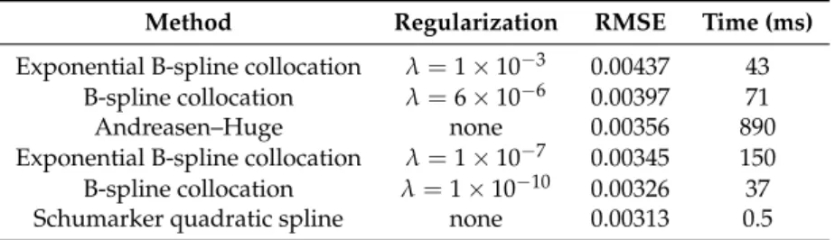
With a small (or zero) regularization parameterλ, the resulting implied probability density possesses many spurious spikes (Figure2a). The use of a larger regularization parameterλ, during the non-linear minimization of the objectiveEdescribed in Equation (18), helps smoothing the spikes, but it increases the RMSE slightly (see Table1).
Table 1. Root mean square error (RMSE) of the collocation method implied volatilities against the market implied volatilities of the TSLA 1 m options as of 18 June 2018.
Method Regularization RMSE Time (ms)
Exponential B-spline collocation λ=1×10⁻³ 0.00437 43
B-spline collocation λ=6×10⁻⁶ 0.00397 71
Andreasen–Huge none 0.00356 890
Exponential B-spline collocation λ=1×10⁻⁷ 0.00345 150
B-spline collocation λ=1×10⁻¹⁰ 0.00326 37
Schumarker quadratic spline none 0.00313 0.5
In Table1, we also compute the RMSE with a simple convexity preserving quadratic spline (Schumaker 1983) on the filtered market option prices (Equation (23)). This interpolation leads to a positive and piecewise-constant probability density. On convex prices, the interpolation is exact. The RMSE is thus purely due to the filtering of the market quotes by quadratic programming.
Andreasen and Huge (2011) propose a different non-parametric arbitrage-free volatility interpolation, where a discrete local volatility is calibrated to market option prices in a one-step finite-difference discretization of the forward Dupire partial differential equation. The number of free parameters corresponds effectively to the number of quotes, as in the spline collocation, and their technique will also tend to overfit. It is known to lead to a nearly exact interpolation on arbitrage-free option prices. It does however not lead to a more accurate representation of the market implied volatilities than the B-spline collocation with a small regularization constant. The corresponding implied probability density also possesses spikes.
0.000 0.001 0.002 0.003 0 200 400 600 Strike Probability density Regularization constant 1×10⁻¹⁰ 6×10⁻⁶
(a)Probability density implied by the prices obtained with a calibrated B-spline collocation
40 60 80 100 120 0 200 400 600 Strike Implied v olatility in % Implied volatility B−spline collocation Market
(b)Volatility smile implied by the prices obtained with B-spline collocation with regularizationλ=6×10⁻⁶
Figure 2.Implied probability density and implied volatility for the B-spline collocation, calibrated to 1 m TSLA options.
The B-spline collocation is not only at least as accurate as the technique ofAndreasen and Huge(2011) on this example, it is also significantly faster. In the latter, the involved finite difference grid must be relatively large (we used 800 points) and the corresponding tridiagonal system must be solved for each set of piecewise constant volatilities considered by the minimizer. Furthermore, the B-spline collocation offers a continuous interpolation of the option prices. In the technique of
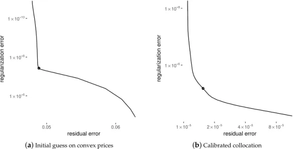
Andreasen and Huge(2011), options prices are given only at the finite difference grid points. Another careful4arbitrage-free interpolation must be used to compute the price in between grid points. Finally, the B-spline collocation offers the ability to tune the probability density smoothness against the RMSE. The optimal regularization parameter can be found using the L-curve method (Hansen 1992). On Figure3b we plot the L-curve for the calibrated B-spline collocation, that is the regularization
4 In practice, we solve the Fokker-Planck forward PDE instead of the Dupire forward PDE, and then integrate the option payoff
on the known probability density as inHagan et al.(2014);Le Floc’h and Kennedy(2017) in order to obtain arbitrage-free
norm against residual norm, in logarithmic scale, or equivalently, the second sum against the first sum of Equation (19), varying the regularization parameterλ. For most regularization techniques, such a curve is L-shaped, because, on linear problems, the regularization norm is a strictly decreasing function of the regularization parameterλ, and the residual norm is a strictly increasing function ofλ. A good regularization parameter will achieve a good compromise between the two errors, and will correspond to a regularized solution near the “corner” of the L-curve. On non-linear least-squares problems in general, the regularization and residual norms will not be strictly monotonic, they will however be nearly monotonic and the L-curve method may still be applied (Aster et al. 2018, p. 241). Our choice λ = 6×10⁻⁶ is the point located in the corner of the L-curve (see Figure 3b). Performing multiple calibrations to find the optimal regularization parameter, following one of the algorithms ofHansen and O’Leary(1993), may be time-consuming. An alternative is to apply the L-curve method to the B-spline initial guess based on the convex option prices5(Figure3a).
1×10+6 1×10+8 1×10+10 0.05 0.06 residual error regular ization error
(a)Initial guess on convex prices
1×10+6 1×10+8 1×10⁻⁵ 2×10⁻⁵ 4×10⁻⁵ 8×10⁻⁵ residual error regular ization error (b)Calibrated collocation
Figure 3. L-curves of the B-spline corresponding to the initial guess, and the calibration result on TSLA options.
7.2. Exponential B-Spline
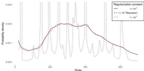
The exponential B-spline initial guess does not preserve the first moment. As a consequence, its calibration tends to be less stable than the calibration of the regular B-spline. The choice of initial guess plays then an important role, and the inclusion of the regularization in the calculation of the exponential B-spline initial guess is particularly important. The RMSE in the implied volatilities is comparable to the one obtained by the Andreasen and Huge technique, and is larger than the RMSE of the regular B-spline collocation (Table1). In spite of the larger error, the implied probability density is not as smooth as the one implied from the regular B-spline collocation (Figure4). A smoother initial guess, such as the constant Bachelier volatility, is then preferable.
0.000 0.001 0.002 0.003 0 200 400 600 Strike Probability density Regularization constant 1×10⁻³ 1×10⁻³ (Bachelier) 1×10⁻⁷
Figure 4.Implied probability density for the exponential B-spline collocation, calibrated to 1 m TSLA options, with different regularization constants.
7.3. Starting from Arbitrage-Free Prices
It is also interesting to take the filtered convex option prices (from Equation (23)) as a basis to compare the different techniques. We expect the RMSE to be lower, eventually zero, if the interpolation is exact at the market strikes. For example, the convexity-preserving Schumaker quadratic spline results in an RMSE of exactly zero (but the associated implied probability density is a staircase). The B-spline collocation results in an RMSE of around 0.0005 without regularization constant. This is lower than the RMSE produced by the Andreasen–Huge technique. In theory, their technique should be able to attain a lower RMSE, but the number of strikes, and thus the number of constants to optimize is relatively large on our problem and this creates difficulties for the numerical optimization. The collocation on an exponential B-spline leads to an RMSE similar to the one obtained with the Andreasen–Huge technique (Table2). Of course, with a small regularization constant, the corresponding probability density possesses many spikes and is not very practical.
Table 2. Root mean square error (RMSE) of the collocation method implied volatilities against the implied volatilities of the TSLA 1 m options as of 18 June 2018, based on convexity adjusted prices.
Method Regularization RMSE Time (ms)
Exponential B-spline collocation λ=10−3 0.00287 35
B-spline collocation λ=6×10⁻⁶ 0.00239 39
Exponential B-spline collocation λ=10−7 0.00118 160
Andreasen–Huge none 0.00112 890
B-spline collocation λ=10−10 0.00042 78
Schumaker quadratic spline none 0 0.02
On other market data, for example, options on NFLX from July 2018, the same conclusions can be drawn.
8. A More Extreme Example—Wiggles in the Implied Volatility
Jäckel(2014) shows that undesired oscillations can appear in the graph of the implied volatility against the option strikes when the option prices are interpolated by a monotonic and convex
spline. Table A2 in AppendixA presents a concrete example6. Here, the option quotes are not direct market quotes, but the solution of a sparse finite difference discretization of a local stochastic volatility model: the market never quotes so far out-of-the-money option prices. His data has a few interesting properties:
• some of the option prices are extremely small: the interpolation must be very accurate numerically.
• the option prices are free of arbitrage. In theory, an arbitrage-free interpolation can be exact.
• a cubic spline interpolation on the volatilities or the variances, often used by practitioners, is not arbitrage-free.
• a convexity preservingC1-quadratic, orC2-rational spline results in strong oscillations in the implied volatility.
The interpolation proposed in (Jäckel 2014) possesses unnatural spikes at the points of clamping, in particular, the implied density is not continuous.
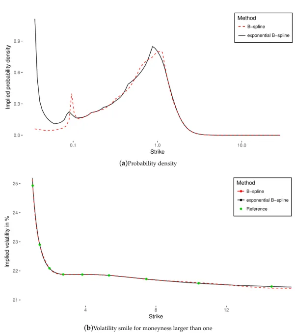
For this example, the B-spline collocation leads to a relatively large RMSE when compared to Andreasen–Huge method. As a consequence, we can see an oscillation of small amplitude in the corresponding implied volatility for large strikes (Figure5b). This is very mild compared to the spline interpolations presented in (Jäckel 2014). The higher error is mostly located in the left wing. The exponential B-spline collocation results in a much lower RMSE, albeit still larger than the Andreasen and Huge technique (Table3). The volatility implied by the exponential B-spline collocation does not oscillate.
The optimal implied probability density is relatively smooth, but possesses a few visible modes (Figure5a). This makes the monotonic polynomial collocation of Le Floc’h and Oosterlee(2019) ineffective, even when using a high degree polynomial. Polynomials of degree seven and higher lead to a RMSE larger than one vol point.
Table 3. Root mean square error (RMSE) of the collocation method implied volatilities against the implied volatilities of TableA2in AppendixA.
Method Regularization RMSE Time (ms)
Septic polynomial none 1×10⁻² 230
B-spline λ=10−12 2×10⁻⁴ 10
Exponential B-spline λ=10−7 6×10⁻⁵ 10
Andreasen–Huge (800 nodes) none 1×10⁻⁶ 25
Andreasen–Huge (3200 nodes) none 9×10⁻⁸ 67
Schumaker convex spline none 0 0.02
It is possible to obtain a better fit with the B-spline collocation with a better choice of knots, for example, if we compute the knots implied by the calibrated B-spline collocation, and calibrate one more time. In Table4, we denote this technique as “Best”. It improves significantly the accuracy on the example of Peter Jäckel, but not on the filtered and non filtered TSLA market option quotes, where the different choices for the initial knots lead to a very similar RMSE.
On Peter Jäckel’s example, the optimal implied probability density is relatively smooth everywhere, and especially for strike moneyness larger than one. Figure6 shows however that the probability density implied by technique ofAndreasen and Huge(2011) exhibits a staircase shape when zoomed-in. This is due to the interpolation in between the finite difference grid nodes. In contrast, the probability density implied by the (exponential) B-spline collocation stays very smooth, and is continuous by construction.
0.0 0.3 0.6 0.9 0.1 1.0 10.0 Strike
Implied probability density
Method B−spline exponential B−spline (a)Probability density 21 22 23 24 25 4 8 12 Strike Implied v olatility in % Method B−spline exponential B−spline Reference
(b)Volatility smile for moneyness larger than one
Figure 5.Implied probability density and implied volatility for the spline collocations of the market data of TableA2in appendixA.
Table 4. Root mean square error (RMSE) of the collocation method implied volatilities starting the calibration with the Bachelier, the convex, or the “best” initial guess, and using a small regularization constant.
Market Data Collocation Method Bachelier Convex Best
Peter Jäckel B-spline 0.00063 0.00025 0.00001
Exponential B-spline 0.00016 0.00006 0.00003
TSLA raw B-spline 0.00330 0.00326 0.00322
Exponential B-spline 0.00343 0.00345 0.00343
TSLA convex B-spline 0.00054 0.00042 0.00034
0.01 0.02 0.03 2.5 2.6 2.7 2.8 2.9 3.0 Strike Probability density Interpolation Andreasen−Huge
Exponential B−spline collocation
Figure 6.Implied probability density for the exponential B-spline collocation and Andreasen–Huge techniques, for strike moneynessK∈[2.5, 3.0], calibrated to the market data of TableA2in AppendixA. The B-spline has a knot located atK=2.679.
9. Conclusions
The monotonic B-spline and exponential B-spline collocations allow a more flexible arbitrage-free representation as compared to the monotonic polynomial collocation. They can capture multi-modal distributions well. In practice, when the goal is to fit market option prices, we have shown that is important to add a regularization during the optimization in order to stabilize the calibration and produce a smooth implied probability density, and we have described which regularization is appropriate.
We have also presented a simple non-parametric technique to de-arbitrage a set of option prices, which may be used independently of the B-spline collocation method.
In some specific cases, such as the example fromJäckel(2014), the outcome of the B-spline calibration may be dependent on the choice of the initial fixed knots. In the latter example, the exponential B-spline collocation behaved better, however.
On actual market options quotes, corresponding to various equity or equity indices, we did not observe this strong dependence on the choice of initial knots. We observed a quality of fit in terms of implied volatilities similar to or better than the best non-parametric arbitrage-free methods, such as the technique ofAndreasen and Huge(2011). Compared to the latter, the spline collocation has the advantage of providing a natural continuous interpolation and extrapolation. The technique from Andreasen and Huge is based on a fine discretization of the problem, and requires an additional careful arbitrage-free interpolation scheme to compute the prices for option strikes not placed on the discretization grid. The B-spline collocation is also less computationally intensive, as the Andreasen and Huge technique mainly works well on a dense grid, typically composed of thousand points or more.
An additional interesting property of the exponential B-spline representation is the simple analytical expression we obtain for the price of a variance swap. The latter is a linear combination of the B-spline parameters. This allows including the market prices of variance swaps very easily into the calibration and thus obtaining a better representation of the wings of the implied volatility.
Finally, the B-spline and exponential B-spline collocations can be used directly to price exotic derivatives within the collocated local volatility model ofGrzelak(2016).
We leave for further research the definition of an algorithm for an automatic selection of the best B-spline knots, as well as an extension to B-splines of order four.
Author Contributions: Conceptualization, F.L.F. and C.W.O.; methodology, F.L.F. and C.W.O.; software, F.L.F.; writing–original draft preparation, F.L.F.; writing–review and editing, C.W.O.; visualization, F.L.F.; supervision, C.W.O.
Funding:This research received no external funding.
Conflicts of Interest:The authors declare no conflict of interest.
Appendix A. Market Data
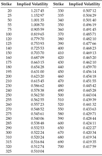
Table A1. Implied volatilities against strikesKfor TSLA options expiring on 17 January 2020 as of 15 June 2018. This corresponds to a maturityT=1.59178 and the forward isf =356.73.
Strike Implied Volatility Strike Implied Volatility
20 1.217 45 330 0.507 12 25 1.152 97 335 0.504 29 50 1.001 35 340 0.501 40 55 1.008 70 350 0.496 19 75 0.905 59 360 0.491 45 100 0.819 65 370 0.485 71 120 0.779 70 380 0.482 10 125 0.753 93 390 0.477 66 140 0.725 53 400 0.468 23 150 0.703 70 410 0.469 13 160 0.687 09 420 0.465 20 175 0.663 15 430 0.462 10 180 0.654 28 440 0.459 70 195 0.631 00 450 0.456 14 200 0.623 20 460 0.454 18 210 0.615 45 470 0.451 55 230 0.586 62 480 0.445 42 240 0.578 38 490 0.445 28 250 0.562 50 500 0.443 04 255 0.562 55 510 0.439 39 260 0.557 23 520 0.441 32 270 0.548 52 550 0.433 63 275 0.545 61 580 0.429 71 280 0.540 06 590 0.428 44 285 0.538 48 600 0.424 11 290 0.532 53 650 0.422 27 300 0.522 24 670 0.420 34 310 0.520 24 680 0.419 34 315 0.516 84 690 0.419 35 320 0.512 74 700 0.417 59 325 0.510 04
Table A2.Implied volatilities against moneynessKFfor an option of maturityT=5.0722, corresponding to the example 1 ofJäckel(2014).
Moneyness Implied volatility
0.035 12 0.642 41 0.049 10 0.621 68 0.068 62 0.590 58 0.095 92 0.553 14 0.134 08 0.511 40 0.187 41 0.466 70 0.261 96 0.420 23 0.366 17 0.373 30 0.511 82 0.327 56 0.715 42 0.285 11 1 0.249 33 1.397 78 0.228 97 1.953 80 0.220 86 2.730 99 0.218 76 3.817 33 0.218 74 5.335 80 0.218 43 7.458 29 0.217 20 10.425 07 0.215 74 14.572 00 0.214 62 20.368 49 0.214 11 28.470 74 0.214 58 References
Andreasen, Jesper, and Brian Norsk Huge. 2011 Volatility interpolation. Risk24: 76. [CrossRef]
Andersen, Martin S., Joachim Dahl, and Lieven Vandenberghe. 2013. CVXOPT: A Python Package for Convex Optimization. Available online:abel.ee.ucla.edu/cvxopt(accessed on 22 January 2019).
Aster, Richard C., Brian Borchers, and Clifford H. Thurber. 2018. Parameter Estimation and Inverse Problems. Amsterdam: Elsevier.
Breeden, Douglas T., and Robert H. Litzenberger. 1978. Prices of state-contingent claims implicit in option prices. Journal of business51: 621–51. [CrossRef]
Carr, Peter, and Dilip Madan. 2001. Towards a theory of volatility trading. InOption Pricing, Interest Rates and Risk Management, Handbooks in Mathematical Finance. Cambridge: Cambridge University Press, pp. 458–76. Carr, Peter, and Roger Lee. 2009. Robust Replication of Volatility Derivatives. Available online: www.math.
uchicago.edu/~rl/rrvd.pdf(accessed on 22 January 2019).
Corlay, Sylvain. 2016. B-spline techniques for volatility modeling. Journal of Computational Finance19: 97–135. [CrossRef]
De Boor, Carl. A Practical Guide to Splines. New York: Springer, vol. 27.
Demeterfi, Kresimir, Emanuel Derman, Michael Kamal, and Joseph Zou. 1999. More than you ever wanted to know about volatility swaps. Goldman Sachs Quantitative Strategies Research Notes41: 1–56.
Dupire, Bruno. 1994. Pricing with a smile. Risk7: 18–20.
Eilers, Paul H. C., and Brian D. Marx. 1996. Flexible smoothing with B-splines and penalties. Statistical Science 11: 89–102. [CrossRef]
Gatheral, Jim. 2004. A Parsimonious Arbitrage-Free Implied Volatility Parameterization With Application to the Valuation of Volatility Derivatives. InPresentation at Global Derivatives & Risk Management, Madrid. Available online:faculty.baruch.cuny.edu/jgatheral/madrid2004.pdf(accessed on 22 January 2019).
Glass, J. M. 1966. Smooth-curve interpolation: A generalized spline-fit procedure. BIT Numerical Mathematics 6: 277–93. [CrossRef]
Grzelak, Lech A., and Cornelis W. Oosterlee. 2017. From arbitrage to arbitrage-free implied volatilities. Journal of Computational Finance20: 31–49. [CrossRef]
Grzelak, Lech A. 2016. The CLV Framework-A Fresh Look at Efficient Pricing with Smile. SSRN 2747541. Available online:papers.ssrn.com/sol3/papers.cfm?abstract_id=2747541(accessed on 22 January 2019).
Hagan, Patrick S., Deep Kumar, Andrew Lesniewski, and Diana Woodward. 2014. Arbitrage-Free SABR.Wilmott 2014: 60–75. [CrossRef]
Hansen, Per Christian. 1992 Analysis of discrete ill-posed problems by means of the L-curve. SIAM Review 34: 561–80. [CrossRef]
Hansen, Per Christian, and Dianne Prost O’Leary. 1993. The use of the L-curve in the regularization of discrete ill-posed problems.SIAM Journal on Scientific Computing4: 1487–503. [CrossRef]
Huynh, Hung T. 1993. Accurate monotone cubic interpolation. SIAM Journal on Numerical Analysis30: 57–100. [CrossRef]
Hyman, James M. 1983. Accurate monotonicity preserving cubic interpolation. SIAM Journal on Scientific and Statistical Computing4: 645–54. [CrossRef]
Jäckel, Peter . 2014. Clamping Down on Arbitrage. Wilmott2014: 54–69. [CrossRef] Kahalé, Nabil. 2004. An arbitrage-free interpolation of volatilities. Risk17: 102–6.
Kanzow, Christian, Masao Fukushima, and Nobuo Yamashita. 2004. Levenberg-Marquardt methods for constrained nonlinear equations with strong local convergence properties. J. Computational and Applied Mathematics 172: 375–97. [CrossRef]
Klare, Kenneth, and Guthrie Miller. 2013. GN—A Simple and Effective Nonlinear Least-Squares Algorithm for the Open Source Literature. Available online: www.netlib.org/misc/gn/GN_ReadMe.pdf(accessed on 22 January 2019).
Le Floc’h, Fabien. 2016. Fast and Accurate Analytic Basis Point Volatility. SSRN 2420757. Available online: papers.ssrn.com/sol3/papers.cfm?abstract_id=2420757(accessed on 22 January 2019).
Le Floc’h, Fabien, and Cornelis W. Oosterlee. 2019. Model-Free Stochastic Collocation for an Arbitrage-Free Implied Volatility, Part I.Decision in Economics and Finance. Available online:link.springer.com/article/10. 1007/s10203-019-00238-x(accessed on 22 January 2019).
Le Floc’h, Fabien, and Gary J. Kennedy. 2017. Finite difference techniques for arbitrage-free SABR. Journal of Computational Finance20: 51–79.
LeVeque, Randall J. 2007. Finite Difference Methods for Ordinary and Partial Differential Equations: Steady-State and Time-Dependent Problems. Philadelphia: SIAM, vol. 98.
Mathelin, Lionel, and M. Yousuff Hussaini. 2003. A Stochastic Collocation Algorithm for Uncertainty Analysis. CR-2003-212153. Hampton: NASA Langley Research Center, pp. 1–16.
Nonweiler, Terence R. 1968. Algorithms: Algorithm 326: Roots of low-order polynomial equations.Communications of the ACM11: 269–70. [CrossRef]
Schumaker, Larry I. 1983. On shape preserving quadratic spline interpolation. SIAM Journal on Numerical Analysis 20: 854–64. [CrossRef]
Stellato, Bartolomeo, Goran Banjac, Paul Goulart, Alberto Bemporad, and Stephen Boyd. 2017. OSQP: An Operator Splitting Solver for Quadratic Programs. arXiv. Available online: http://xxx.lanl.gov/abs/1711.08013 (accessed on 22 January 2019).
Turlach, Berwin A., and Andreas Weingessel. 2007. quadprog: Functions to Solve Quadratic Programming Problems. CRAN-Package. Available online:https://cran.r-project.org/web/packages/quadprog/index. html(accessed on 22 January 2019).
c
2019 by the authors. Licensee MDPI, Basel, Switzerland. This article is an open access article distributed under the terms and conditions of the Creative Commons Attribution (CC BY) license (http://creativecommons.org/licenses/by/4.0/).

![Figure 6. Implied probability density for the exponential B-spline collocation and Andreasen–Huge techniques, for strike moneyness K ∈ [ 2.5, 3.0 ] , calibrated to the market data of Table A2 in Appendix A.](https://thumb-us.123doks.com/thumbv2/123dok_us/10079493.2907973/18.892.154.550.144.425/probability-exponential-collocation-andreasen-techniques-moneyness-calibrated-appendix.webp)