UNIVERSITY OF TARTU
Institute of Computer Science
Computer Science Curriculum
Annett Saarik
Trajectory Reconstruction and Mobility
Pattern Analysis Based on Call Detail
Record Data
Master’s Thesis (30 ECTS)
Supervisor: Amnir Hadachi, PhD
Trajectory Reconstruction and Mobility Pattern Analysis
Based on Call Detail Record Data
Abstract: Up until now, GPS data has been greatly used for collecting highly precise locational data from moving objects including humans. In contrast, mobile phone data is becoming more and more popular in the last few years. The usage of mobile phone data, that is also known as CDR data, has many benefits over the widely used GPS. This means that the methods used for example in GPS trajectory reconstruction, need to have modifications made be compatible with CDR data.
The fact that telecommunication companies have started to cooperate more and share the CDR data with the public is also a boost to the usage of CDR data. The processed and analyzed CDR data can be used to get an overview of crowd movement in different scales, for example traveling inside a city as opposed to between countries. Extracting trajectories from CDR data has numerous com-plications. This is due to the fact that the data might not be continuous and discovering of the starting point of the object in motion is complicated.
The goal of this thesis is to use CDR data in the reconstruction of trajectories made by an anonymous user and to validate the results with GPS data generated in parallel to the CDR data. Reconstructed trajectories can be used for movement analysis and population displacement and would help city planning by optimizing the infrastructures.
Outcomes of this thesis are the reconstructed trajectories based on CDR data and the precisions of final paths. Also, the frequency of CDR events is analyzed in addition to distance distribution. After that the areas that the user visits most frequently are extracted, such as home and work locations.
Keywords: Call detail record, trajectory reconstruction, location data, crowd movement, mobility patterns
Trajektooride taastamine ja inimeste liikumise mustrite anal¨
u¨
us
mobiiltelefoni andmete p˜
ohjal
L¨uhikokkuv˜ote: Tehnoloogiad, mis kasutavad geograafilisi andmeid, on muutu-nud meie igap¨aevaelu t¨ahtsaks osaks. T¨anu sellele on kasvanud asukoha andmete massiliine salvestamine ja kaevandamine. Seni on GPS tehnoloogiad olnud p˜ ohi-liseks geograafiliste andmete kogumismeetodiks. Sellega paralleelselt on populaar-sust kogunud mobiiliandmete kasutamine positsiooni tuvastamiseks ja liikumis-mustrite anal¨u¨usimiseks. Mobiiliandmete (CDR) p˜ohjal trajektooride taastamiseks on vajalik meetodite kohendamine selleks, et tulemused oleksid korrektsed.
T¨anu sellele, et telekommunikatsiooni ettev˜otted on alustanud suuremat koost¨o¨od ja hakanud CDR-andmeid j¨arjest rohkem avalikustama, on mobiiliandmete kasuta-mine mitmetel aladel suurenenud. T¨o¨odeldud mobiiliandmed aitavad anda ¨ ulevaa-det rahvastiku liikumisest erinevates ulatustes. Samal ajal on trajektooride taasta-mine CDR-andmetest kohati raskendatud v˜orreldes GPS-andmetega. Suurimaks probleemiks on algus- ja l˜opp-positsioonide asukoha m¨a¨aramine, mis on veelgi enam raskendatud juhul kui objekt liigub.
Selle l˜oput¨o¨o eesm¨argiks on trajektooride taastamine anon¨u¨umsete kasutajate poolt genereeritud CDR-andmete p˜ohjal. Tulemuste valideerimine GPS-andmetega, mis on loodud paralleelselt mobiiliandmetega ning on vajalik selleks, et m¨a¨arata saadud trajektooride t¨apsust. Loodud trajektoore saab kasutada objektide, seal-hulgas ka inimeste, liikumismustrite anal¨u¨usimiseks ja rahvastiku paiknemise tu-vastamiseks, mis aitab linnade planeerimisel ja infrastruktuuride optimeerimisel. L˜oput¨o¨o v¨aljunditeks on trajektooride taastamine ja t¨apsuse anal¨u¨usimine, lisaks sellele inimese liikumismudelite tuvastamine ja tihedamini k¨ulastatavate asukohta-de iasukohta-dentifitseerimine nagu n¨aiteks kodu, t¨o¨okoht ja poed.
V˜otmes˜onad: Mobiiltelefoni andmed, trajektoori konstrueerimine, asu-koha andmed, rahvastiku liikumine, inimeste liikumise mustrid
Acknowledgements
First, I would like to extend my gratitude to the best supervisor in the world, Dr. Amnir Hadachi for endless guidance, patience and the ability to keep a sense of humour, when I had lost mine. For the last year he has been a solid source of knowledge and wisdom.
I would like to thank my parents, Anu Saarik and Silver Saarik, who always believed in my capabilities even when I did not and supported me in my decision to pursue studies in Tartu University. I am grateful for the work they have done, to give me the life I have now. Without their encouragement and faith, I could not have done it.
Last but not least, I would like to thank Karl Rankla, Mari Krusten, Reimo Rebane and Jenny Holm for helping me by reading and giving valuable advice to improve my work. To the computer science ladies, Olha Shepelenko and Asmar Hasanova, big thanks for the support and for keeping the morale high during the thesis writing.
Contents
Acknowledgements 4 List of Abbreviations 8 List of Figures 9 List of Tables 9 1 Introduction 10 1.1 General view . . . 101.2 Research questions and objectives . . . 11
1.3 Scope . . . 11
1.4 Contributions . . . 11
1.5 Road map . . . 12
2 State-of-the-art 13 2.1 Call Detail Records . . . 13
2.1.1 Relevant issues with CDRs . . . 13
2.1.2 Applications with CDR data . . . 14
2.2 Trajectory data mining . . . 15
2.2.1 Trajectory preprocessing . . . 16
2.2.2 Trajectory data management . . . 17
2.2.3 Trajectory uncertainty . . . 18
2.2.4 Trajectory pattern mining . . . 18
2.2.5 Trajectory classification . . . 19
2.2.6 Applications of trajectory data mining . . . 20
2.3 Human mobility patterns . . . 23
2.3.1 Transportation . . . 23
2.3.2 Urban planning . . . 24
2.3.3 Event detection . . . 25
2.3.4 Semantic analysis . . . 25
3 Calculating the trajectories 28
3.1 Call Detail Records . . . 28
3.2 Technologies applied . . . 30 3.2.1 OpenCellID . . . 31 3.2.2 OpenStreetMap . . . 32 3.2.3 NetworkX . . . 33 3.3 Trajectory preprocessing . . . 34 3.3.1 Cell ID query . . . 34 3.3.2 Geometric center . . . 34
3.3.3 Importing Tartu road data into a network . . . 36
3.3.4 Nearest road . . . 36
3.4 Reconstructing the trajectories . . . 39
3.4.1 Calculating the time intervals . . . 39
3.4.2 Reconstructing paths . . . 39
3.4.3 Cell ping-pong handover problem . . . 40
3.5 Validating with GPS data . . . 41
4 Human mobility patterns 45 4.1 Frequency of CDR events . . . 45
4.2 CDR dispersion over distance . . . 46
4.3 User POI . . . 48
4.3.1 Home and work . . . 48
4.3.2 Additional POIs . . . 49
5 Conclusion 52 5.1 Future work . . . 53
List of Abbreviations
API Application Programming Interface
BTS Base transceiver station
CDR Call Detail Record
CI Cell ID
CS Computer Science
EVP Exceptionally Visited POIs
GPS Global Positioning System
GSM Global System for Mobile Communication
GU Geographical Unit
ITS Intelligent Transportation Systems
JSON JavaScript Object Notation
KNN K-Nearest Neighbor
LAC Location Area Code
LCSS Longest Common Subsequence
MCC Mobile Country Code
MMPP Markov modulated Poisson process
MNC Mobile Network Code
MVP Mostly Visited POIs
OSM OpenStreetMap
POI Point of Interest
SMDR Station Messaging Detail Record
List of Figures
1 Overview of trajectory mining methods. . . 16
2 Antenna and four cell coverage areas (polygons) surrounding it. . . 29
3 Cell tower locations in Estonia from OpenCellID API. . . 31
4 OSM road data of Tartu shown in NetworkX structure. . . 33
5 Calculated centroids with coverage areas (polygons). The centroids are in green and polygons are in blue. . . 35
6 Cell coverage area centroid and nearest node in OSM. The centroids are in blue and nearest nodes are in yellow. . . 38
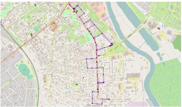
7 Trajectory reconstruction based on CDR data. Trajectory points are in pink and GPS locations are shown as blue rectangles. . . 42
8 Trajectory reconstruction based on CDR data. GPS trajectory is in red and CDR trajectory is in blue. . . 43
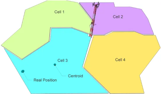
9 Cell 3 centroid and the real starting position of the object. . . 44
10 Histograms of event frequencies for the entire dataset. . . 46
11 Histograms of distance distribution for the entire dataset. . . 47
12 Cell tower connections. . . 48
13 Work and home areas shown in blue polygons. . . 49
14 Frequently visited areas. . . 50
15 POI inside the frequently visited area. Visited area is shown within a blue polygon line and POI are in green dots. . . 51
16 Event frequency during weekdays. . . 61
17 Event frequency during weekends. . . 62
18 Distance distribution during weekdays. . . 63
19 Distance distribution during weekends. . . 64
List of Tables
1 Example of CDR data used in this thesis. . . 292 Notation to the Vincenty’s inverse formula. . . 36
1
Introduction
The introduction chapter gives an insight about positioning and how this thesis work is contributing into the field of Intelligent Transportation Systems (ITS). The research that has been conducted is focused on investigating the use of mobile phone data also known as Call Detail Records (CDR) in reconstructing trajectories and extracting human mobility patterns.
1.1
General view
The usage of geospatial data in people’s everyday lives has become more frequent over the years. Geospatial data is a dataset that includes geographic data. Spatial data makes mundane tasks easier by helping to make travel plans from short trips to the market, to longer more elaborate plans, to travel across country borders. This data can be presented with location attributes such as latitude and longitude, address, postal code, street name etc. In some cases the information is represented by more complex data types and structures.[PT14]
One option to collect enormous amounts of geospatial data is from Global Po-sitioning System (GPS) devices, such as mobile phones, which are used frequently by people in their daily lives. The growth over the last 15 years in the number of mobile cellular services subscribers is remarkable. In the year 2015 the number of unique cellular (GSM) subscribers has increased to around 4.7 billion.[mob16]
There are some disadvantages with collecting GPS data, such as the user must enable the settings for GPS tracking and this drains the battery of the device faster. This is not the case in collecting CDR data. CDR is a record of every transaction a mobile subscriber makes. These transactions include calls, messaging or even just waking the mobile phone from sleep mode. This means that every time, when a mobile phone is connected to an antenna, CDRs are made continuously and stored by the telecommunication companies. Companies save the records for billing the subscriber for their use of the telecommunication services.[ict16]
In this thesis CDRs are acquired from a mobile application developed by the distributed systems group in University of Tartu, Computer Science Institute. This data is used to calculate the possible location data (latitude and longitude) of the
mobile user at the moment of the CDR creation. From these sets of latitude and longitude it is possible to construct trajectories of users from a certain starting point A to destination point B. Using these trajectories helps in understanding complex movement patterns that mobile phone users make in their daily lives. These patterns can give an overview of the complicated migration of crowds in small and large scale. Small scale meaning commuting to workplace or traveling around the user’s residential area. Large scale is more sophisticated movement from non-urban to urban areas and vice versa also migration to foreign countries.
1.2
Research questions and objectives
The goals of this thesis is to compute user trajectories from CDR data, validate them with the GPS data that was collected in parallel, to assess the legitimacy and precision of the CDR trajectory reconstruction results. An additional goal is to examine individual user’s mobility patterns and areas of significance.
• Is it possible to to reconstruct human generated trajectories based on CDR data and what is the accuracy compared to GPS data?
• What are the individual user’s mobility patterns and places of significance based on CDR data?
1.3
Scope
In this thesis, CDRs that are used in the trajectory reconstruction and further pattern analysis are generated by mobile users, who have the mobile application, developed by distributed group, mobCollector installed and have agreed to share their data for academic purposes. Data is collected inside Estonia country borders. In total 3721 CDR and 682 GPS records were used.
1.4
Contributions
Methodologies used in this thesis are mainly built on data analysis: understand-ing, preprocessunderstand-ing, cleanunderstand-ing, modeling and individualizing the data. The main objectives that are targets in this thesis are:
• acquiring cell ID location data from OpenCellID;
• calculating the cell coverage area polygon centroids;
• processing road data;
• discovering the nearest nodes from the road data;
• reconstruction of the trajectories based on CDR data;
• CDR event distribution analysis;
• CDR distance dispersion analysis;
• detecting frequently visited locations.
1.5
Road map
The road map gives a brief introduction to the structure and chapters of this thesis.
Chapter 2. Gives an overview of the current research that has been done in the related fields of this thesis. Subjects such as description of CDR data, trajectory reconstruction and human mobility patterns are covered.
Chapter 3. Includes a more detailed sight into the geospatial data used in this thesis and a thorough description of the steps and calculations made to generate the trajectories based on CDRs.
Chapter 4.Is about analyzing one anonymous user’s event and distance distribution in addition to identifying most frequently visited places.
Chapter 5. Conclusion of the thesis and description the possible future work is in the last chapter.
2
State-of-the-art
This chapter gives an overview of research that has been conducted in the related CS fields. CDR data, trajectory reconstruction and crowd movement have been part of many academic research papers and this chapter will examine the possible overlapping of these subjects.
2.1
Call Detail Records
CDRs are records that are generated by the mobile subscriber of a telecommuni-cation company. These records are generated, when the mobile phone is connected to an antenna and the user has interacted with their mobile phone. Different in-teractions are called events. The records can consist of various data and usually are not identical among the providers. There is no universal format implemented for this data and the providers can choose the content of the records themselves. Given the sensitivity of information in CDRs, it is a good practice to anonymize the identifying fields in the records. This means the names and/or mobile numbers are removed from the data and commonly replaced with unique integer numbers for specific subscribers.
2.1.1 Relevant issues with CDRs
Because CDR data is very different from GPS data it presents multiple challenges in processing it. Some of them are:
• Temporal sparseness - The CDRs are generated when the user interacts with their mobile phone. A large number of mobile users make infrequent calls and messages or the records made are periodically irregular. This is not the case with GPS generated data.
• Spatial sparseness - The location recorded with an event is the location of the cell tower and this brings the spatial sparseness into the CDR data.
• Non-routine events - Regular events like going to work or home are easier to detect. Non-regular events like football or some other social events are not
part of the usual routine trajectories and therefor are more unpredictable. [DPG+15]
The privacy concerns with using and processing CDR data are an additional chal-lenge. Even when names and mobile phone numbers are anonymized and all identifying data linked to the user is removed, there is an increasing awareness of the re-identification possibility. For example, identifying the specific field of work or a profession of a mobile subscriber from a seemingly random CDR dataset. By clustering one specific user’s two most visited areas it is possible to discover significant locations by checking, if it is a residential area for home area.[Pul13]
2.1.2 Applications with CDR data
There are many possible development opportunities for mobile phone network data. Benefits in smart city planning and transportation are a given and presented in one of biggest projects with mobile phone data in fixing bus routes in the city of Abidjan. The telecommunication company released 2.5 billion CDRs to research the possibilities of improving the bus routes and scheduling in the city. The research included extracting frequent sequential patterns from the stops made and locating users’ home and work areas, resulting in 65 improvement suggestions and two new added routes. This optimized the system enough for a 10 percent decrease in travel time for citizens.[BCDL+13]
In addition to transportation system planning, CDRs can also be used in dis-aster response. This was researched with data collected after the Haiti earthquake in 2010. It is a natural response to any disaster to flee from the affected areas, therefore finding out exactly how people react and move after catastrophes can help in organizing and managing first responders. Disasters also include infec-tious disease outbreaks and man-made hazards, for example terrorist attacks or industrial accidents.[BLT+11]
There have been many projects made in health research and disease prevention with mobile phone data. One of most significant studies was with quantifying malaria outbreaks in Kenya. Around 15 million mobile subscribers’ data was acquired for a time period of one year, to map their regional travels. Together with the malaria transmission model, which shows the rate of infection, specific
ares were located, where the probability of malaria spreading was higher.[WET+12]
Social science research can also benefit from applying mobile phone data. In 2012 census data and CDR were used to research and find recognizable patterns in various social groups of the subscribers. In this project census data consisted of socioeconomic information from the same area as the CDRs are collected from. Around 10 million subscribers’ data was acquired from 12 cities[FMV12]. Results showed a strong correlation between the socioeconomic level of a specific subscriber and the expenses, physical distance with the contacts and geographical areas where people travel. Another research in Republic of Cˆote d’Ivoire was conducted to use CDRs to determine and map poverty lines in that area. Greater amount of mobile communication between subscribers and larger range of calls are an indicator for larger prosperity. As a result poverty lines of eleven regions of Cˆote d’Ivoire were estimated.[SMC13]
2.2
Trajectory data mining
Spatial trajectories are location sequences generated by moving objects, such as humans, vehicles or even animals. As a result of rapidly advancing tracking tech-nologies and mobile computing, processing and generating trajectories from that data is becoming more prominent. Research in trajectory reconstruction and data mining is extensive. Most of the studies inspect different techniques for trajectory computing with location data like GPS or CDR. In the research paper ”Trajectory Data Mining: An Overview” by Dr. Yu Zheng, there is detailed description of tra-jectory construction methods. The five major subjects tratra-jectory preprocessing, indexing, uncertainty, pattern mining and classification are introduced in the next four chapters.[Zhe15]
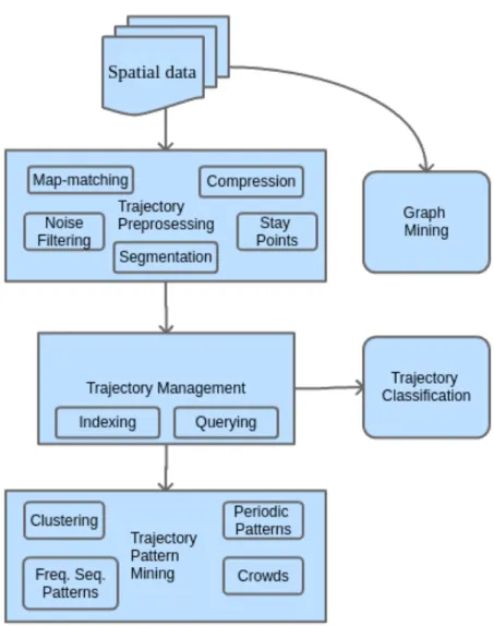
Figure 1 gives a simple overview of the process flow in trajectory data mining and subjects covered in this thesis. Spatial data in the beginning of the chart can represent both GPS and CDR data. In this thesis it represents CDR data collected from volunteer users.
Figure 1: Overview of trajectory mining methods.
2.2.1 Trajectory preprocessing
Before using the trajectory data there are numerous problems that need addressing in order to start working with the data. More substantial issues concerning trajec-tory preprocessing can be covered with five suggested solution methods explained in more detail in the list below.
• Noise filtering. When working with trajectory data some location measure-ments may be incorrect by several (hundred) meters. These deviations in the data depend on the technology used and the physical objects that interfere
with the signal near the true location. To remove the inaccurate points from the trajectory a median filter can be used. The filter algorithm calculates medians between a point n and its n−1 predecessors in a period of time. If the next median differs more than the agreed upon allowed error, it is a noise point. The median filter is not efficient for sparse trajectory data. This means the filter cannot be used with CDRs. For scattered dataKalman
filter or particle filter can be used. Kalman filter takes a motion model into account and estimates states like speed with assuming linear models. The particle filter algorithm relaxes these assumptions and therefore is a less efficient algorithm.[LK11]
• Stay points. Some points in a trajectory are more significant than other, for example opposed to noise points there are also stay points. These points represent locations where an object has stayed for a longer period. When calculating data generated by humans, the stay points can be shops, malls, restaurants etc.[Zhe15]
• Compression. To minimize memory storage and computing time there are two compression methods. The offline method reduces the trajectory after it has been completely generated and the online method, which compresses trajectories instantly as an object moves.[LK11]
• Segmentation. For a very detailed analysis on trajectory segmentation it is split into smaller parts. Segmentation can be based on time, the shape of the trajectory or semantic meaning (walking, driving) of the parts.[Zhe15]
• Map-matching. Last preprocessing method is map-matching, which converts a sequence of latitude and longitude data to a road segment where the object generated corresponding points.[Kru11]
2.2.2 Trajectory data management
Searching and querying over enormous sets of trajectory data is time consuming. Indexing increases the efficiency of these queries and makes trajectory data storage management easier. Queries are divided into two types K-Nearest Neighbor (KNN)
and range. KNN query recovers the top-K trajectories that are positioned inside the minimum accumulated distance range. In order to use KNN queries a distance (or similarity) function, that is based on minimum bounding rectangles between two trajectories, needs to be determined. Two concepts that are acquired from string matching can be implemented in function Longest Common Subsequence (LCSS) and Edit Distance. Range queries are also referred to as distance metric, meaning the evaluation of distances between two trajectories. Range queries fetch segments of the trajectory that are within a previously defined spatial range. The result of the query can be used to verify a feature within the segment such as object speed.[DXZZ11]
2.2.3 Trajectory uncertainty
As a result of spatial data sparseness uncertainty occurs in trajectories. As ob-jects move constantly, but the number of recorded location points are limited, the locations of objects between two documented points are ambiguous. This problem arises with CDR data more frequently than in GPS.[Tra11]
2.2.4 Trajectory pattern mining
In trajectory pattern mining there are four distinguishable categories that observe and inspect patterns from one or more trajectory. These categories include moving together patterns, trajectory clustering, sequential patterns and periodic patterns.
• Moving together patterns. As the name suggests, this category discovers ob-jects that move together in a certain period of time. These patterns are used in species migration, military surveillance and traffic event detection. It can be used to detect possible bottlenecks in city road systems during rush hours. The groups of objects traveling together are called flocks and swarms. Flock is a group that is moving simultaneously in at leastk period of time. Swarm is a composed version of a flock leaving out the time requirement.[JYJ11]
• Trajectory clustering. Combining together objects, that have same paths at some point in their movements, is called trajectory clustering. The paths are
split into segments and objects with similar ones can be identified by cal-culating the distances between two complete trajectories. Micro-and-Macro Clustering approach is also used to first find clusters in very small subsets and grouping small micros together to generate bigger macro clusters.[JYJ11]
• Sequential patterns. When objects travel in homogeneous paths through points and during similar times, sequential patterns can be identified. The sequences share same locations and comparable travel times, although the se-quence does not have to be consecutive. As an example view the trajectories
A and B inFormula 1. A:l1 1.5h −−→ l2 1h −→l7 1.2h −−→ l4. B :l1 1.2h −−→l2 2h −→l4, (1)
where l is a location. In the example A and B share the same sequence l1 → l2 →l4 although they are not consecutive. Discovering these patterns
can enhance the accuracy of next location calculation, estimating similarities, trajectory compression and travel recommendation.[JYJ11]
• Periodic patterns. Searching and identifying recurring events results in pe-riodic patterns. These patterns are made by objects that generate similar trajectories when certain time period has passed. For instance people going to the market on weekends or gift-shopping before holidays. For detecting these patterns two stage detection method is used. Density algorithm is im-plemented to find popular locations among objects. Considering the result, trajectories are reconstructed into time series with values in and out as a status of the moving object at a certain popular location. The final stage is to generate summaries from partial movement sequences using hierarchical clustering algorithm.[JYJ11]
2.2.5 Trajectory classification
Separating trajectories (or parts of it) by difference in status is called trajectory classification. Various states include movement, such as walking, biking, driving or using public transport. Adding these semantic descriptions to trajectories adds
value in context aware computing. Trajectory classification process is broken down to three major stages:
1. Using segmentation methods to divide trajectories into sections. 2. Extracting characteristics from all sections.
3. Generating a model to identify every section.[Zhe15]
A research project based on GPS data categorizes object’s trajectory by trans-portation mode [ZLWX08]. The main classes were driving, biking, walking and taking public transport and the reason for them is that a person can take multiple transportation method during one trajectory. The segments are identified with a class through Decision Tree Classifier. The principal is that movement information about heading change, stop and velocity adjustment rate are extracted and read into the Decision Tree after that results are classified the a model is implemented in the Decision Tree.[ZCL+10]
2.2.6 Applications of trajectory data mining
Numerous fields, such as transportation, urban planning, environment, energy, so-cial, business and public safety, use trajectory mining applications. In this chapter urban planning and transportation applications are explained in detail [MT16]. For a regular smartphone user more familiar applications might be path discovery in transportation such as Google Maps1 or any alternative, for instance WikiMapia
Map2, MapQuest Map3 or Waze Map4. The main applications for trajectory data
mining are explained in detail in the list below.
• Path discovery. Is the most common trajectory mining application, it is also very popular among users in their daily lives. Finding the most rea-sonable route for travels has been the focus point of many research projects [DYGD15]. As users’ preferences for route attributes vary the path discov-ering algorithm also differ. As some people prefer shorter distance lengths 1www.google.ee/maps
2www.wikimapia.org/ 3www.mapquest.com 4www.waze.com/livemap
for smaller gas consumption others only care about the time spent on the travels. More sophisticated path detections techniques also take into ac-count the traffic and even weather. In ITS various research examines how to update the paths simultaneously with real time data from various sensing technology.[Zel98]
• Destination prediction. Is linked to path discovery and it is found that hu-man mobility and movement is profoundly regular and therefore predictable in high precision. In a research paper about restraints of human mobility the prediction accuracy rate was 93% [SQBB10]. Large number of location based applications use destination prediction to send advertisements or special of-fers to potential clients. Recording past trajectories to databases improves destination predictions. When a user is traveling through a regular path des-tination corresponds with the final location in the past trajectories.[CLC10]
• Movement behavior analysis. Trajectory calculations gives many ways of analyzing object’s movement and finding occurring patterns. One substan-tial research is conducted in determining patterns between sociodemographic groups based on age, wealth, gender, educational level and wealth [RBdM+13]. Another research paper identifies groups, such as animals, humans and ve-hicles, traveling together in time intervals. The movement behavior for this type of event is called gatherings and are found by large dataset indexing, searching and updating issues. Gatherings can be celebrations, parades, protests, traffic congestions and other public assemblage. The five main characteristics of gatherings are:
1. number of participants is high;
2. participants arrange a compressed group; 3. event should occur in a certain time interval; 4. geometric attributes of groups stay the same;
5. there is a number of participants, who stay in the group at any time for a certain interval.[ZZYS13]
In the research a sizable dataset, consisting of location data, is collected from taxicabs in Beijing [ZZYS13]. Research in discovering object’s, in this case
a human’s, rationality to enter a certain point of interest (POI). POI can be any potential stopping point from shopping malls, restaurants and to bus stops, hospitals.[LQW15]
• Group behavior analysis. Examines clusters of objects, that are likely to generate between groups, during motion. These clusters develop due to their social behavior and to discover them techniques from Chapter 2.2.4
are used. Research has been conducted in trajectory modeling to describe the movement patterns in shifting groups. These patterns include events like parades, protests and traffic bottlenecks.[ZZYS13]
• Urban computing. Obtaining data from sources such as sensors, devices, vehi-cles, buildings, humans and analyzing it to find better solutions for problems in the city. Using data to solve these issues, like air pollution, energy con-sumption and traffic bottlenecks, in cities is called urban computing [FZ16]. The usage of trajectory data in urban development has many benefits, for example processed trajectories can be used to optimize public transportation schedules and routes, also in planning and building new roads. The identifi-cation of regions, such as residential, business and eduidentifi-cation, in cities helps urban planners to understand the complexity of cities.[ZCWY14]
• Understanding trajectories. Making sense of trajectory data without seman-tic descriptions can be problemaseman-tic and to simplify this attributes are added to segments of trajectories by modeling data with specific features. More fre-quently used semantic attributes are divided by the mean of transportation used, such as walk, drive, bus[PSR+13]. Some location applications require
a semantic attribution of locations for instancework orhome [LCC12]. An-other method to make the trajectory data understandable is to use visual analytics methods such as map-matching, graphs, images.[AA13]
2.3
Human mobility patterns
Human mobility has been mentioned several times in Chapters 2.1 and 2.2.4. This chapter gives a more detailed analysis about human mobility pattern dis-covery and presents prominent research in the field. This chapter is divided into four subchapters: transportation, urban planning, event detection, semantic anal-ysis. All of these subchapters cover a specific field, which uses mobility pattern applications.
2.3.1 Transportation
Detecting and analyzing human mobility patterns from location data has numerous benefits in transportation, such as rescheduling public transport when needed and discovering traffic anomalies. Planning and building streets and infrastructure is also moderately connected to transportation but in this paper, will be covered in
Chapter 2.3.2. This chapter gives an overview of techniques for processing CDR data to improve the transportation infrastructure in a certain region.
Understanding the human mobility in a city and detecting POIs for the purpose of improving transportation is crucial. There is regularity in the trajectories and time in human mobility, that lead to the following characterizing aspects:
• movements of individuals are summarized in as a set of points, where they stay the longest time;
• places visited only once are time consuming;
• humans travel between points based on temporal distance;
• most frequently visited POIs are home and work.[PJZ+16]
Traffic anomalies such as congestion, accidents, bottlenecks can greatly affect nor-mal traffic flow in cities. To identify unusual events from mobile data metrics, such as trip rates, travel distance and travel time need to be calculated [CMS+16]. In the research project about determining these values trajectories of individuals were mostly used.[GHB08]
Observing the traffic flow in cities, at a crowd level can give additional insight to problems. Big datasets of trajectories are an effective base for understanding
mobility patterns at society-wide range. For example a study in Milan identified roads most used by the morning and evening commuters in addition to the exact times when traffic bottlenecks developed in the city.[GNP+11]
2.3.2 Urban planning
Using spatial data in urban planning can increase the understanding of urban dy-namics and human movement flows. Analyzing location data allows urban planners to monitor the fast changing urban dynamics. Also to detect upcoming trends in movement of the citizens[DL99], which can be very time consuming and difficult using traditional surveys, such as questionnaires.[RFPW06]
Approximately 15 million CDRs were collected around city of Morristown to get an overview of residents’ daily travels. The geographical areas surrounding the city, where workers live are given a semantic namelaborshed. In contrast, areas where people would frequently visit the community location such as bars and restaurants are calledpartyshed. By grouping residents by their preferred activities around the city it is possible to model typical flow of the residents between different parts of the city.[BCH+11]
Human mobility is complex, but almost never random. The movement of people is affected by their needs, commitments and social obligations. As an outcome of these factors human mobility patterns show regularity in daily (weekly, monthly, etc) movements. These regularities can be characterized by defining the
Relevance Ratio and POI [NSL+12] of the user u under observation, such as in
Formula 2.
RR(P OI, u) = dvisit(P OI, u) dtotal(u)
(2) where dvisit(P OI, u) is the sum of days that the location has been visited and
dtotal(u) is the sum of all days in the user data. These locations are categorized
into three classes Mostly Visited POIs (MVP), Occasionally Visited POIs (OVP) and Exceptionally Visited POIs (EVP), by frequency of visits.[JZGR16]
2.3.3 Event detection
Event is considered a substantial activity not regular in daily human patterns. To discover these type of events, object’s history and regular movements are taken into account and any sort of deviations from regular paths are detected. After that Poisson and exponential distribution models are used. With these steps it is possible to characterize regular behavior and recognize anomalous events. If the thresholds of frequencies and spans are smaller than for any event that occurred, it can be categorized as an anomaly.[ZD12]
Alternative method for detecting unusual events, from more than one object, is more suitable for CDR data, because of the issues described in Chapter 2.1.1. The process is divided into multiple steps, firstly CDRs are received and split into clusters, after that crowds are detected from sequences of clusters. Afterwards constraints are verified for each crowd detected and a tag (unusual) is added to it. One or more crowds construct an unusual event.[DPG+15]
Definition 2.1. (Crowd) A crowdC is
CCtm, CCtm+1, ..., CCtn that represents
consecutive clusters with three constraints. Movement, because number of points visited needs to be over one. Durability, number of consecutive clusters is bigger than threshold. Commitment, number of participants in any given moment is greater than the threshold.
Unusual events were detected from CDRs in Abidjan, Cˆote d’Ivoire. Markov modulated Poisson process (MMPP) was modified to detect hourly and daily be-havioral anomalies from spatial data. As result unusual events found from mobile data correlated with events such as protests, holidays and major sport events that actually occurred in the area. Additionally, analyzing mobile data as a time series gives better output in tracking masses during movement.[GISL16]
2.3.4 Semantic analysis
From object spatial data such as CDRs most visited places, also known as POI, are attainable as mentioned in previous chapter. Giving these POI a semantic meaning adds more personal information about the object under observation. Two places with the highest frequency of visits often arehome andwork. Finding other semantic locations from trajectory data is more complex.
The two issues with combining the location data to a semantic meaning, are obtaining the spatial data and after that labeling the locations with semantic meaning. To obtain most occurring points from location data, clustering (parti-tioning, density-based, time-based) algorithms are used. The disadvantage with these techniques is that the result is a geographic point with a radius, but does not include a semantic meaning. Another approach uses hierarchical algorithm compiled with both time-based and density-based clustering.[LCC12]
Definition 2.2. (Location point) Is P from the trajectory as a pairp= (lat, lon). Where lat is the latitude andlon is the longitude.
Definition 2.3. (Trajectory) Is a sequence of location points with added times-tamps, represented as traj = (p0, t0), ...,(pn, tn) , where p is a location and t is
the timestamp.
Definition 2.4. (Visit point) Is a location with two timestamps, defined asvp= (p, tin, tout), where p is the location and tin is arrival time and tout is departure
time.
Definition 2.5. (Physical place) Is a cluster of location points, represented as pp= (vp1, ..., vpn), where vp1 and vpn are nearby.
The time-based algorithm checks, ifvpis located in the cluster of points already generated, and compares the time intervals and distances. If the time period is greater and distance is less than the tolerated threshold, it is in fact a visit point. [LCC12]
In another research same types of clustering algorithms were used to find vari-ous user groups from CDR data. The main attributes for clusters, were time (day, week) and distance (Euclidean distance). All of the unique users’ CDR data was aggregated into 1-hour blocks by day of the week. Results show that it is possible to identify student mobile users by their daily and hourly usage pattern. The other group identified is commuters, who use their mobile phones more during the morning and evening rush hours.[BCH+]
In comparison, location data can be nowadays collected from social sites, such as Twitter5. This was tried in a project for mining users mobility patterns within
urban context. As a result it was possible to identify most frequent route pat-terns between famous London landmarks. The outcome can be used to generate personalized travel recommendations for tourists.[CFT16]
Because mobile phones are ubiquitous nowadays and present in high and low income households, CDR data can be used to recognize and analyze needs and habits of various groups. In a project conducted in Latin America mobile phone data was combined with socio-economical census data, collected by the National Statistical Institute, during a period of five years and divided into Geographical Units (GUs). CDR data was grouped into polygons using Voronoi diagrams and then merged with GUs. Results display correlations among various socio-economic levels. Larger distances of the call maker and receiver means a higher economic background of the users. Accuracy of these calculations is R2 ≈0.82.[FMV12]
2.4
Conclusion
To summarize, there is extensive work done in the fields of trajectory data mining and human patterns, but many problems are still unsolved. Thanks to open data movements gaining support, many telecommunication companies have started to take steps towards sharing their CDR data. This gives more opportunities to investigate human mobility more extensively and with less financial losses. At the moment CDR trajectory reconstruction methods are not highly accurate. This is due to the fact that origin and destination point recovery is difficult and usually not very precise.[LWB+13]
3
Calculating the trajectories
This chapter introduces the methods and technologies used in the processing of CDR data that has been collected by a mobile application developed by the dis-tributed systems group at the University of Tartu, Computer Science Institute. In parallel to CDRs, GPS data was also gathered in the same time period. This enables the verification of data legitimacy in trajectory reconstruction covered in
Chapter 3.5. Additionally to CDRs multiple resources were used to collect and filter data. In Chapter 3.1 there is a detailed description of CDR data, after that inChapters 3.2.1 and 3.2.2two additional services are introduced that were used in the trajectory reconstruction process.
3.1
Call Detail Records
GSM is an international mobile phone standard that provides connection services for subscribers. The GSM system consists of base transceiver stations or BTSs. Each system covers a geographical area that is called a cell coverage area (polygon). BTS enables the gathering of information about every GSM device that is in connection. This type of data is known ascall detail records or CDRs (alsostation messaging detail record or SMDR). Information collected in CDRs can include:
1. metadata;
2. phone number of the mobile subscriber or when anonymized, user id (SID); 3. timestamp;
4. cell location data such as MCC, MNC, LAC, CI (descriptions in Chapter 3.2.1);
5. event type (i.e. handover, pickup).
In addition to information in the list above, telecommunication operators can include or remove fields as they choose. CDRs are described as passive location data compared to GPS data, which is considered active. CDRs are generally formatted in XML (eXtensible Markup Language) based tagging schema that is
defined by the operators. CDR data is used to generate invoices for subscribers of telecommunication companies and to analyze network traffic.[cdr13]
Table 1: Example of CDR data used in this thesis.
ID SID tascii CGI
1 100562421962333 2016-10-16 09:00:39.853 248-2-1002-54412 2 100562421962333 2016-10-16 09:00:53.227 248-2-1002-54415 3 100562421962333 2016-10-16 09:00:58.546 248-2-1002-56593 4 100562421962333 2016-10-16 09:01:10.524 248-2-1002-54412 Example of a CDR used in this thesis, is shown in Table 1. Irrelevant fields, to this thesis, were left out of the table. User generated CDRs are represented as a row and contains SID, timestamp (tascii) and CGI that includes location data divided by a dash.
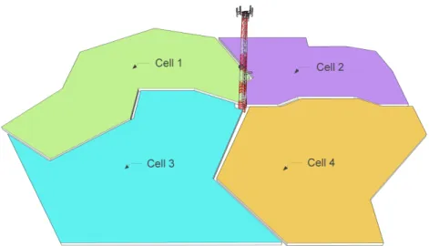
Figure 2: Antenna and four cell coverage areas (polygons) surrounding it.
Figure 2 is an illustration of one antenna that can four coverage areas (poly-gons). In real life the antenna can have multiple cell towers mounted on it. The polygons are irregular and can overlap each other. In more complex cases, one coverage area can wrap another entirely.
3.2
Technologies applied
Various libraries and software was used in this thesis. Reading in and processing CDR data was made by using Python programming language6library named
Pan-das7. Pandas is an open source library offering high-performance, easy-to-use data
structures and data analysis tools. Jupyter Notebook8 was used as a programming
environment because it contains live code, equations, visualizations and supports Python and all the libraries used in this thesis. Other technologies used in this thesis:
• OpenCellID9 - explained in Chapter 3.2.1;
• OpenStreetMap10 - explained in Chapter 3.2.2;
• NetworkX11 - explained inChapter 3.2.3;
• QGIS12 - free open source software for creating, editing, analyzing geospatial
information. In this thesis QGIS was used to visualize CDR paths;
• Numpy13- package for scientific computing with Python was used to conduct
multiple calculations with location data and distances;
• Matplotlib14 - Python library for generating high quality graphs and plots;
• Requests15 - the HTTP library for Python was used to make queries to
various services;
• Geopy16 - Python client for numerous geocoding web services was used in
trajectory reconstruction; 6www.python.org 7www.pandas.pydata.org 8www.jupyter.org 9www.opencellid.org 10www.openstreetmap.org 11www.networkx.github.io 12www.qgis.org 13www.python.org 14www.matplotlib.org 15www.python.org 16www.geopy.readthedocs.io
• Scipy17- Python-based system of open-source software for mathematics,
sci-ence and engineering was used in various computations.
3.2.1 OpenCellID
OpenCellID is an open-source community collaboration project that aims to col-lect and document GPS locations of cell towers and share this data. Volunteer users can upload and download spatial data through a Location API (Application Programming Interface). OpenCellID data together with CDR data can be used to replace GPS as a tracking method with cell IDs, which helps to save device battery power and to track a device in a building, where GPS is not available.
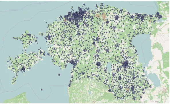
Figure 3: Cell tower locations in Estonia from OpenCellID API.
In this thesis four fields of data was used to identify the cell ID. An example of location data is inTable 1 where cell tower data is in column CGI. When splitting the column by dash, the fields are:
• MCC - Mobile Country Code represented as a integer number (Estonia is 248);
• MNC - Mobile Network Code represented as ainteger number;
• LAC - Location Area Code of the operator network;
• CI - Cell ID.
Accuracy of the data may vary, because OpenCellID is open-source and community based service. This means that some API queries got inaccurate results back or no result at all and these errors were removed. InFigure 3all the cell tower positions are shown inside Estonia. In urban areas there are clearly more towers to serve bigger number of users as opposed to rural areas.
3.2.2 OpenStreetMap
OpenStreetMap (OSM) is an online service that collects world’s geographic data and distributes it for free. The service has about 20 000 active users, who volunteer to assemble and upload geographic data. All maps generated with collected data are adjustable by users and can be used as they see fit. The data can be downloaded in the format of XML. The XML files include tags:
• node is a geographical point on earth with latitude and longitude as at-tributes;
• way is an ordered sequence (list) of nodes that all together make up a portion (polyline) of a road or a street;
• relation is a connection to model logical (usually local) or geographic rela-tionships between objects.
OSM data includes additional data about road segments, for example max speed, bus stops etc. In addition to the data, OSM has multiple functions to query and manipulate spatial data. OSM has an API for querying and saving data. [HW08] For this thesis the road data is downloaded by boundary box query to the API. For example the downloaded road data for Tartu had 24655 nodes and 27933 ways.
3.2.3 NetworkX
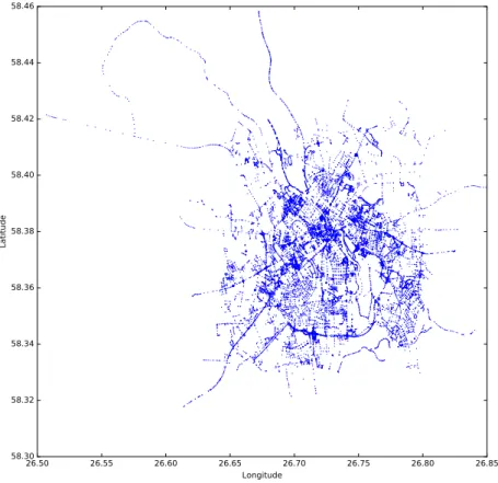
For the purpose of searching and processing OSM road data faster, nodes, ways and relations were read into a network structure with NetworkX. NetworkX is a Python language software package for creating, manipulating and studying structures and functions of the network, in addition it is possible to read in and store data as a graph. While reading OSM data into structure, every node and way was identified with an ID number from the original OSM road data file. In Figure 4 nodes in
26.50 26.55 26.60 26.65 26.70 26.75 26.80 26.85 Longitude 58.30 58.32 58.34 58.36 58.38 58.40 58.42 58.44 58.46 La ti tu de
Figure 4: OSM road data of Tartu shown in NetworkX structure.
Tartu are shown in a graph structure using NetworkX. Nodes have id, latitude and longitude as data. As seen in the figure, nodes make up a network that resembles Tartu’s road system.
3.3
Trajectory preprocessing
As mentioned in the previous chapters, multiple technologies were used to recon-struct the trajectories from original CDR data. In this section all the steps in data processing are described in detail and intermediate results are visualized.
3.3.1 Cell ID query
OpenCellID API is used to search and download cell IDs in Estonia. CDR data does not include latitude and longitude parameters, because of this querying the OpenCellID API is necessary. When an API query is successful JSON format file is downloaded as a response. An example of a JSON file for one query is below.
{ ” l o n ”: 2 4 . 7 7 4 6 7 2 1 9 2 3 0 7 6 9 4 , ” l a t ”: 5 9 . 3 7 7 4 6 3 3 0 7 6 9 2 2 9 5 , ”mcc”: 2 4 8 , ”mnc”: 2 , ” l a c ”: 1 , ” c e l l i d ”: 5 5 1 4 5 , ” a v e r a g e S i g n a l S t r e n g t h ”: 1 0 , ” r a n g e ”: 1 4 1 5 7 , ” s a m p l e s ”: 2 6 , ” c h a n g e a b l e ”: t r u e , ” r a d i o ”: ”GSM” }
Listing 1: OpenCellID API query response in JSON.
As can be seen from the example above, desired cell tower latitude and longitude attributes are included in the JSON file. Due to the fact that OpenCellID data is gathered by volunteer users, the data may have errors or be missing in some cases. Around one third of the results were empty.
3.3.2 Geometric center
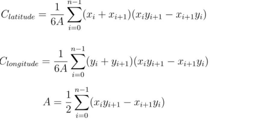
Because the cell ID latitude and longitude are not the cell center, the geometric centroid from a polygon is calculated and the total number of the vertices is un-known in the polygons. Formulas (3),(4) and (5) were used to find the latitude
Clatitude and longitude Clongitude of the center point of the polygon. Clatitude = 1 6A n−1 X i=0 (xi+xi+1)(xiyi+1−xi+1yi) (3) Clongitude= 1 6A n−1 X i=0 (yi+yi+1)(xiyi+1−xi+1yi) (4) A= 1 2 n−1 X i=0 (xiyi+1−xi+1yi) (5)
InFormula (5) polygon’s areaAis calculated. InFormulas (3) and (4) latitude and longitude coordinates is calculated by using the intermediate area result and number of n vertices (x0, y0),(x1, y1), ...,(xn−1, yn−1).
Figure 5: Calculated centroids with coverage areas (polygons). The centroids are in green and polygons are in blue.
Calculated centroids are shown inFigure 5with the cell coverage area polygons. As can be seen from the figure, some cell areas are overlapping others and some even hide multiple smaller areas underneath.
3.3.3 Importing Tartu road data into a network
Nearest road to the centroid is calculated using OSM service that was described in
Chapter 3.2.2. Using the API, tiles of OSM with a boundary box are downloaded and processed. Boundary box query consists of attributes, such as minimum longi-tude, minimum latilongi-tude, maximum longitude and maximum latitude. Due to the fact that downloaded OSM files are very big (OSM file of Tartu has 24655 nodes and 27933 ways) a script was made to download road data according to latitude and longitude points. Two different methods were used to calculate bounding box attributes to download road data. Calculating bounding box from one point and two points. The last one was used to reconstruct path between two CDR points. The XML files of road data were read into a complex network with NetworkX. Road data in a network structure enables nearest node and path search.
3.3.4 Nearest road
To find the nearest road OSM data is used to find the closest node to the centroid. Vincenty’s inverse formula [Vin75] was used to calculate distances, because of the high accuracy of the calculations with geographic points. The high precision is achieved by calculating geodesic distances on ellipsoids, this gives results within a one millimeter error radius. The high accuracy is important when reconstruction the trajectories and also in mobility pattern analysis. Formula of the Vincenty’s inverse equation is shown below and also the notations are explained inTable 2 .
Table 2: Notation to the Vincenty’s inverse formula.
a radius at equator, 6378137.0 meters in WGS-84 f flattening of the ellipsoid, 1/298.257223563 in WGS-8 b= (1−f)a radius at the poles, 6356752.314245 meters in WGS-84 U1 =arctan[(1−f)tanΦ1] reduced latitude
U2 =arctan[(1−f)tanΦ2] reduced latitude
L=L2 −L1 difference in longitude of two points
λ1, λ2 longitude of the points on auxiliary sphere
α1, α2 forward azimuths at the points;
α azimuth at the equator
s ellipsoidal distance between two points
sinσ=p(cosU2sinλ)2+ (cosU1sinU2−sinU1cosU2cosλ)2 (6)
cosσ = sinU1sinU2+ cosU1cosU2cosλ (7)
σ = arctan sinσ
cosσ (8)
sinα= cosU1cosU2sinλ
sinσ (9) cos2α = 1−sin2α (10) cos(2σm) = cosσ− 2 sinU1sinU2 cos2α (11) C = f 16cos 2α 4 +f(4−3 cos2α) (12) λ=L+(1−C)fsinασ+Csinσcos(2σm) +Ccosσ(−1 + 2 cos2(2σm)) (13)
When λ has been assembled using Formulas 12 and 13 to the wanted degree of precision (1012 corresponds to 0.06mm). Assembling λ is done by iterating over
Formulas(6 to11. After all that proceed to evaluate the following formulas.
A= 1 + u 2 16384 4096 +u2−768 +u2(320−175u2) (14) B = u 2 1024 256 +u2−128 +u2(74−47u2) (15) ∆σ=Bsinσncos(2σm) + 14B cosσ −1 + 2 cos2(2σm) − 1 6Bcos(2σm)(−3 + 4 sin 2 σ) −3 + 4 cos2(2σm) o (16) s =bA(σ−∆σ) (17)
, where ∆σ is a result of Formulas 14, 15and 16. u2 = cos2αa
2−b2
After all that the result can be calculated by Formulas 19 and 20. α1 = arctan
cosU2sinλ
cosU1sinU2−sinU1cosU2cosλ
(19)
α2 = arctan
cosU1sinλ
−sinU1cosU2+ cosU1sinU2cosλ
(20) Explanations to variables in Vincenty’s inverse formulas are inTable 2. In this thesis WGS84 is used in distance calculations and visualizations in QGIS. WGS84 is an Earth-centered reference system and geodetic datum. WGS84 projection is based on a set of constants and parameters that describes the Earth’s size, shape.
Figure 6: Cell coverage area centroid and nearest node in OSM. The centroids are in blue and nearest nodes are in yellow.
Results of the nearest node search from OSM road data are shown in Figure 6. Blue points are the calculated centroids from polygons and yellow are the nearest nodes from the road data.
3.4
Reconstructing the trajectories
After completing all of the steps in preprocessing, path reconstruction is possible. Firstly the shortest path between two nearest node points, that are in chronological order, are calculated. With the length of shortest path a cutoff is calculated and used to find paths between two nodes with depth-first search. This is covered in mored detail inChapter 3.4.2. To choose the final path from intermediate results, time intervals are calculated in Chapter 3.4.1 and compared to timestamps of two CDRs from the original data and the closest time interval is the resulting trajectory.
3.4.1 Calculating the time intervals
Time intervals are used to find closest time to the CDR timestamps. Two different times were calculated to find the most accurate path. The average car driving time and the average walking time for previously generated paths using depth-first search. The speed limits were extracted from road data using the OSM service. When data about the legal speed limits was missing, it was set as 50 km/h (city limit) and 90 km/h (highway limit) for driving and 5 km/h for walking. After calculating the result of estimation times for paths, they were compared to the starting point time and destination point time. The path with the closest estimation time was chosen as the trajectory.[LV11]
3.4.2 Reconstructing paths
Paths are generated by first finding the shortest path between two nodes. After that using length of the shortest path to run depth-first search with a cutoff. Be-cause of the fact that a smartphone can ping-pong between cell towers and connect multiple times to one cell tower even when not in movement, there might be mis-leading data in CDRs. These type of double nodes were filtered out from CDRs during the path reconstruction process, to reduce inaccuracies of path generation.
p r o c e d u r e DFS i t e r a t i v e (G, s t a r t , end , c u t o f f ) : l e t S be a s t a c k S . push ( s t a r t ) w h i l e S i s n o t empty v = S . pop ( ) i f S i s s m a l l e r o r e q u a l t o t h e c u t o f f : i f s t a r t i s n o t l a b e l e d a s d i s c o v e r e d : l a b e l s t a r t a s d i s c o v e r e d f o r a l l e d g e s from s t a r t t o end i n G. a d j a c e n t E d g e s ( s t a r t ) do S . push ( end )
Listing 2: Pseudocode of the depth-first search with a cutoff.
In Listing 2, the cutoff if-statement is used before going through the graph nodes and edges. Intermediate results from depth-first search were saved and time intervals were attached to them. After this, time periods were compared and the closest one was resulting path.
3.4.3 Cell ping-pong handover problem
While processing the CDRs for the trajectory reconstruction an anomaly in the spatial data was discovered. For some sequences of CDRs, multiple cell towers reoccurred numerous times. This problem is called the cell tower ping-pong han-dover problem, which means that when the user is located between two cell towers the connection can be passed from one tower to another, due to network traffic fluctuations. In trajectory reconstruction, these double cell towers were removed to get more accurate results. This was done by going through the sequence of cell towers and comparing patterns of three last cell towers to the next ones. When the patterns matched, double occurrences were removed.
3.5
Validating with GPS data
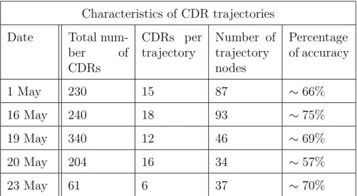
As mentioned previously, GPS is considered an active tracking method and CDR a passive one. In this thesis GPS location data was used to verify the results of the trajectory reconstruction. CDR characteristics, such as total number of CDRs, CDR per reconstructed trajectory, total number of OSM nodes per trajectory and the percentage of accuracy of the reconstructed path are covered in Table 3. The accuracy percentage is calculated by splitting the CDR trajectories into road segments and dividing the accurate number of segments with the total number of segments in the trajectory.
Apercentage = Saccurate Stotal ·100 (21)
In Formula 21Apercentage is the correctly reconstructed trajectory the percentage,
Saccurate is the number of road segments that are equal to the GPS trajectory and
Stotal is the total number of road segments in the path.
Table 3: Table of the processed CDR characteristics.
Characteristics of CDR trajectories Date Total
num-ber of CDRs CDRs per trajectory Number of trajectory nodes Percentage of accuracy 1 May 230 15 87 ∼66% 16 May 240 18 93 ∼75% 19 May 340 12 46 ∼69% 20 May 204 16 34 ∼57% 23 May 61 6 37 ∼70%
In Table 3 five datasets of CDRs are shown, separated by date, that were used to create the overview of CDR trajectory reconstruction accuracy. First dataset might have a lower accuracy because the number of CDRs was somewhat lower, but competed to the fourth dataset, it was located near the city border of Tartu and because lower cell towers the accuracy is lower. Second dataset has a
much higher percentage than others. This could be because the area where the trajectory was did not have many roads. This mean only one or two paths could be generated between two simultaneous CDRs and the correct one was chosen from the results more often. Fourth dataset gave the most inaccurate result. This might be because the CDR in this dataset were more sparse than in others and this made the trajectory error bigger. Accuracy in the fifth dataset is one of the highest, but not as high as in the second one. This might be due to the fact that the number of CDRs is much lower.
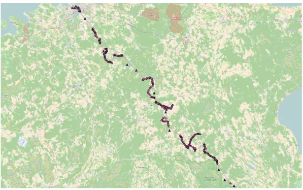
Figure 7: Trajectory reconstruction based on CDR data. Trajectory points are in pink and GPS locations are shown as blue rectangles.
Trajectory reconstruction is shown inFigure 7, for CDR dataset of 19th of May, outside the city of Tartu. Reconstructed path nodes are pink and GPS positions are represented with blue triangles. The path is not continuous and breaks multiple times. Also the trajectory seems to go along numerous side roads and not go along the Tallinn-Tartu highway in a straight line. This result is expected, because in the reconstruction phase object’s real starting position can be different from the cell coverage area centroid. In cases where the object starts movement somewhere near the cell polygon edge, the difference in the calculated and real starting point
can be up to hundreds of meters. In Figure 9 that situation is displayed in cell number 3. This difference in real positions and the centroid affects trajectory reconstruction less in urban areas, because the number of antennas and cell areas is increased. This means that the coverage areas are smaller and close together. This decreases the amount of side roads in the final trajectories and the paths are more accurate. The overall accuracy of the trajectory reconstruction in this thesis is ∼67.4%.
Figure 8: Trajectory reconstruction based on CDR data. GPS trajectory is in red and CDR trajectory is in blue.
InFigure 8reconstructed CDR trajectory is illustrated. The path seems to take many side streets and this is because of the fact that object’s real position and the polygon centroid are not int the same location. There is method for trying to fix this problem usingKalman filters and identifying if the cell is a stay, bypassing or a jump cell and by using these identifiers the real position of the user is calculated with a higher accuracy in stay cases, while in bypassing it is lower.[BHLV15]
4
Human mobility patterns
In this thesis individual user mobility patterns are investigated. In Chapers 4.1
and 4.2 the distribution of user generated CDR events and distances traveled are visualized with time intervals in histograms. To find these patterns in the frequency of the CDR events and the distribution of distances traveled many methods from
Chapter 3, such as using road data from OSM and calculating distances. After that the user’s most frequently visited POIs are identified. In the last chapter CDR cell tower connecting issue is described. The inspected CDRs start from the date 16th of October, 2016 and end in 24th of November, 2016. In total there were 3721 CDRs.
4.1
Frequency of CDR events
Visualization of the CDR event frequencies gives an overview of time periods when the user is most active during the day or week. In Figures 10a and 10b the frequency of the CDR events is shown during workdays and weekends. The number of users events over business days is a lot higher than in weekends. This might be due to the fact that the user works during the week and weekends are leisure time. The first peak in Figure 10a starts around 9 a.m. and ends around 11 a.m, these are the usual commuting to work hours. There is another smaller peak in the lunch time. The biggest peak is during the after office hours from 6 to 7 in the evening, when the user might leave work. There is a smaller peak around 9 p.m., which might indicate some leisure activity for the user. The weekends in
Figure 10b have far less activity and the day starts from 9 a.m. to 11 a.m. with the first peak. Overall the events in weekends are evenly distributed and low. In
Figure 10c the frequency of events are shown by weekdays. The busiest days of the week are Tuesdays and Saturdays. Weekend days have a lot less activity, with Sundays having the smallest frequency of events. In Appendix 5.1 the daily event frequencies of the weekend days are shown. Mostly, the daily histograms conform the overall patterns.
(a) Events per weekdays (b) Events per weekends
(c) Events per weekday
Figure 10: Histograms of event frequencies for the entire dataset.
4.2
CDR dispersion over distance
Plotting the distances of the CDR events in chronological order gives an overview of the times when the user is travels the most distances during the day or week. In Figures 11a and 11b the distance dispersion is shown during workdays and weekends. There are many similarities between the event and the distance distri-bution histograms. The user moves a lot more during weekdays than weekends. In weekdays there are three noticeable peaks. The smallest is from 8 a.m. to 9 a.am., which can be the time interval when the user travels to work. Second one is 4 p.m. and the third one 7 p.m. These hours might be when office workers
usually goes home from work and complete other daily obligations (e.g. shopping, visiting friends). In the evening at 9 p.m. there is a peak, which can indicate to recreational activities. The peak at 1 a.m. is very unusual. Figure 10c confirms that the user travels more during the weekdays and less during weekends. The daily distance distribution is shown in Appendix 5.1. The daily frequencies in the Figure 19are similar to the overall distance distribution during the weekends, which shows that the user does not travel a lot in the days off from work.
(a) Distances per weekdays (b) Distances per weekends
(c) Distances per weekday
4.3
User POI
To find the user’s POI the CDRs were analyzed. In the data there were 883 unique cell IDs that represent sell towers the user had been connected to at some point of the time. InFigure 12a all of the connections are shown and in Figure 12bthe 18 most frequently connected towers are shown. Around 763 towers had connections less than 10 times, which means these areas were most likely visited only once. This means that these cell towers were used, when the user was in motion.
(a) All the cell tower connections. (b) Most popular cell towers.
Figure 12: Cell tower connections.
4.3.1 Home and work
The most frequently connected cell towers were analyzed to find the home and work areas of the user. FromFigure 12bthe ten first cell locations were investigated, to find the area where the user most likely lives and works. Most frequently visited cell location polygons (cell coverage areas) were extracted and visualized. The cell coverage areas that were very close together or even overlapped were considered one area of interest. Area with the most frequently visited cell ID is considered to be the area where the user lives. Because there was insufficient location data for four of the most frequently visited cells additional tasks had to be made. To confirm the home and work place hypothesis the timestamps were extracted and compared. The cell tower that was consistently connected to first in the mornings and last in the evenings was considered the home location and the second area
was the place of work. The resulting home and work areas are shown inFigure 13, where the user’s home seems to be in the south part of Tartu, in an area called Karlova. Because the original home area was very large, topographical attributes were considered, to crop the area to be even more precise. For example the Tartu river and big shopping center were left out, because there are not any residential areas in this region. In addition, the workplace seems to be in Tartu city center. Due to the fact that there are many polygons overlapping around the work area, there can be other POI in that area. This hypothesis is further investigated in
Chapter 4.3.2.
Figure 13: Work and home areas shown in blue polygons.
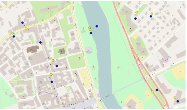
4.3.2 Additional POIs
To detect user’s other POI the frequently visited areas were furthermore examined and intersections were generated. The overlapping areas represent potential loca-tions, where the user has another POI. The two intersections found are presented inFigure 14awith the color red and the frequently visited areas are blue. The big-ger overlapping area seems to be due to the fact that it is the area, where the user works. Second intersection on the other hand seems to be a POI. To confirm this