In-network Outlier Cleaning for Data Collection in
Sensor Networks
Yongzhen Zhuang and Lei Chen
Hong Kong University of Science and Technology
{
cszyz, leichen
}
@cse.ust.hk
Abstract
Outliers are very common in the environmen-tal data monitored by a sensor network con-sisting of many inexpensive, low fidelity, and frequently failed sensors. The limited battery power and costly data transmission have in-troduced a new challenge for outlier clean-ing in sensor networks: it must be done in-network to avoid spending energy on trans-mitting outliers. In this paper, we propose an network outlier cleaning approach, in-cluding wavelet based outlier correction and neighboring DTW(Dynamic Time Warping) distance-based outlier removal. The clean-ing process is accomplished durclean-ing multi-hop data forwarding process, and makes use of the neighboring relation in the hop-count based routing algorithm. Our approach guarantees that most of the outliers can be either cor-rected, or removed from further transmission within 2 hops. We have simulated a spatial-temporal correlated environmental area, and evaluated the outlier cleaning approach in it. The results show that our approach can effec-tively clean the sensing data and reduce out-lier traffic.
1
Introduction
A sensor network is equipped with thousands of inex-pensive, low fidelity motes, which can easily generate sensing errors. The abnormal unreal sensor readings generated in a temporally or permanently failed sensor is calledoutliers. In many cases, outliers introduce er-rors in sensing queries and sensing data analysis. For example, a Sum query is less accurate if a large value outlier is counted. In addition, transmitting outliers to the sink is useless, adds additional traffic burden to the network, and consumes precious sensor energy without any benefit. Outlier cleaning tries to capture the out-liers, correct or remove them from the data stream. Outlier cleaning in sensor networks is challenging be-cause data are distributed among a large amount of
sensors. It is for sure that outlier detection can be conducted centrally after all the data are collected to the sink. However, it is not energy efficient to transmit outliers, especially when the network size is large. For example, if an outlier is routed through a 15-hop path to the sink, the energy used to transmit this 15-hop datum is wasted. Therefore, in-network outlier clean-ing tries to detect outliers durclean-ing the data collection process as early as possible along the routing path of the data. It either corrects the outlier or removes it from further forwarding. Eventually, an outlier-free data stream is provided to the sensor network appli-cations.
In this paper, we propose an in-network outlier cleaning approach for data collection over sensor net-works. We can correct short simple outliers in 0 hop and removelong segmental outlierswithin 2 hops. We adopt wavelet approximation to correct short, occa-sionally appeared outliers. Since these short outliers are of high frequency, they can be corrected if we use the first few wavelet coefficients to represent the sensing series. An extraordinary advantage of using wavelet representation is that it can greatly reduce the dimension of the sensing data, as a consequence, reduces the energy cost of transmitting these data. If an outlier is a long segmental outlier, we can detect it by comparing its similarity with the neighboring nodes, given the nature that environmental data are spatially correlated [1]. Similarity is measured by Dy-namic Time Warping (DTW) distance, which can cap-ture the shape similarity in the elastic shifting sensing series [2]. The sensing series are routed as before to the sink, using a hop-count based routing algorithm [3]. The detection is conducted within 2 forwarding hops. A sensing series is not forwarded, if it is dis-similar with its network neighbors. Outlier cleaning requires in-network data processing on the individual sensor mote. In sensor networks, it is admitted that data processing is more economical than data trans-mission [4]. The outlier cleaning process adds O(KN) running time on each sensor. In the erroneous sensor network, this energy cost is trivial compared to that of the reduced traffic.
The remainder of this paper is organized as follows: Section 2 provides the background of outlier cleaning in sensor network data collection. In Section 3, we describe our in-network outlier cleaning approach in detail. Section 4 presents the evaluation results. Sec-tion 5 discusses the related work, and we conclude this paper in Section 6.
2
Background and Overview
2.1 Sensor Network
In recent years, wireless sensor networks have been growing as a platform for environmental monitoring in agriculture fields, battle fields, wild forests, coal mine tunnels, and so on [5, 6, 7]. Sensors are massively de-ployed to cover a wide geographical area. They have the capability of sensing the area, performing some computation, transmitting and forwarding the data to a centralized sink node. However, these small sensors, also called motes, have their limitations. Two of the most important ones are the limited battery power and the high transmission cost. These limitations make the design of sensor network data processing challenging. It is commonly recognized that in-network processing (aggregation) is beneficial [8, 9, 10, 11]. Part of the data processing is performed earlier, when the data are still in the network. Notice that the centralized approach processes the data only after all of them are collected to the sink. In in-network processing, each sensor takes up some computation according to the ap-plications (e.g. query processing, data collection, event detection, and so on). The sensors try to compute and send the “aggregated” results to reduce network traf-fic. Since data transmission is the most costly opera-tion in sensors [4], compared with it, the energy cost of in-network computation is trivial and negligible.
2.2 Data Collection
Sensor network applications can be classified into sev-eral categories. One kind of popular applications is query processing, which sends out a SQL-like query to the distributed sensors, and expects them to answer it by sending back the results to a sink node [8]. An-other is event detection, in which a sensing report is triggered not by a query, but by the occurrence of an event [12]. Such an event can be a fire in a forest, a gas leakage in a coal mine, or a flood in an agriculture field. The third kind of applications is data collection, which is considered in this paper. These applications collect the entire sensing data over a long time, and store them centrally in a centralized database. So-phisticated data processing and analysis, which is not suitable to be run in sensors, can be carried out in the central server. Data collection is required in many scientific applications, where a scientist usually wants to record the historical monitoring data of the whole geographical area for his/her research. For example, a research for the cause of a freshet would need soil PH, river level, and humidity data over several years. In
this paper, the design of our outlier cleaning approach is described based on the data collection applications. However, the idea of using wavelet-based outlier cor-rection and neighboring DTW distance-based outlier removal can be modified to apply to query processing and event detection applications without losing gener-ality.
2.3 Outlier Definition
In this paper, outliers of sensing data are referred to as abnormal sensed values that are from out of or-der sensors. The nature of environmental monitor-ing shows that sensmonitor-ing series are always temporally and geographically similar. Thus, outliers are those weird sensor readings that are dissimilar with the oth-ers. More specifically, we define two kinds of outliers based on this observation:
Short simple outlier A short simple outlier is a high frequency noise or error. It is usually repre-sented as an abnormal sudden burst and depres-sion, which is dissimilar to the other part of the same sensing series.
Long segmental outliers A long segmental outlier is the erroneous sensed readings that last for a certain time period. It is unreal and cannot reflect the environmental change of its monitoring area during that time period.
2.4 Outlier Cleaning
Outlier cleaning in this paper means both outlier cor-rection and removal. Inoutlier correction, each sensor tries to correct a sensing series that contains outliers. The outlier value is substituted by a close approxi-mation of the real value. It then sends the corrected sensing data to the sink. On the other hand, outlier removal discards the sensing data that are detected to have outliers, and are largely damaged or considered to have little usage. Intuitively, the two outlier clean-ing approaches should be connected in series. One ap-proach should correct the sensing data first, and the other one should then be used to detect long segmen-tal outliers. It is not valid to simply delete the out-liers, because many of them, containing only a little, short, occasionally appeared outliers are still usable af-ter correction. Every piece of sensing data is valuable in a data analysis. It is only when the outliers in the sensing series are too erroneous to correct, then dis-carding this sensing series becomes the only choice to save transmission power. Mapping into the outlier de-finition above, the short simple outlier is much easier to be corrected, and the long segmental outlier need to be removed when it is not correctable.
2.5 Temporal and Spatial Similarity
The environmental data collected from widely distrib-uted sensors are by their nature similar temporally
and spatially [13]. This temporal and spatial simi-larity has special meaning in outlier cleaning. Given a sensing series, a short simple outlier is easy to be identified by human observation because it is shown as a sudden change and extremely different from the rest of the data. Theoretically, this sudden burst or depression is of high frequency in the frequency do-main. They can be removed by de-noising techniques that transform the data into another domain where the high frequency noise and the low frequency true data can be separated. A long segmental outlier that lasts for a certain time period is not easy to be de-tected by only examining one sensing series, because it is hard to tell whether it is an outlier or the true data are changing in that pattern. However, making use of the spatial similarity of the sensing data, the outlier sensor should stand out when compared with the other sensors that monitor the same area. Here we make an assumption that sensors are largely and redundantly deployed, and each sensing area is moni-tored by several sensors. Therefore, an environmental change in an area will have similar, not necessary the same, effect on all the geographically close sensors.
3
Outlier Cleaning
We propose two outlier cleaning approaches:
1. using wavelet-based approach to correct outliers; 2. using neighboring DTW distance-based similarity
comparison to detect and remove outliers. These two outlier cleaning approaches are intended for in-network data processing within sensor networks. However, they are also applicable to centralized outlier cleaning.
3.1 Outlier Correction
Wavelet analysis has long been acknowledged as an efficient de-noising approach. A time series is trans-formed into the time-frequency domain. The wavelet coefficients represent a gradually refined resolution of the original time series. Most of the energy and infor-mation of the data are concentrated in a small number of coefficients, usually the first few coefficients. The sensing noises and errors are of high frequency and reside in high-order coefficients. Therefore, the true data and outliers, which are a kind of noise, can be separated in the wavelet space.
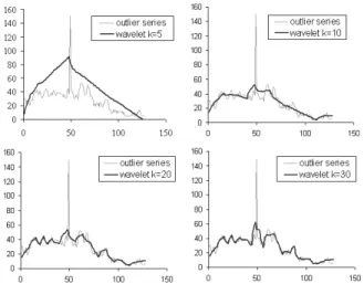
In outlier cleaning, simple short outliers can be cor-rected by wavelet de-noising. Figure 1 shows an ex-ample of using 5, 10, 20, or 30 wavelet coefficients to represent a sensing series with 128 points, which has an outlier at the 48thpoint. We can observe that the
fewer the coefficients used, the smoother and coarser the wavelet restored sensing series. Choosing an ap-propriate number of coefficients, 10 or 20, we can re-move the outlier while keeping a close approximation of the original sensing series.
Figure 1: Outlier correction (Using k= 5, 10, 20, or 30 wavelet coefficients to represent the sensing series. The gray curve is the sensing series with an outlier occurring at the 48th point. The bold curve is the restored sensing series.)
In addition, wavelet transform also acts as a di-mension reduction method. Transmitting the selected wavelet coefficients instead of the original sensing se-ries can reduce data traffic by more than a magnitude. Moreover, wavelet transform, like DWT, only takes O(n) running time, which is a reasonable computa-tional complexity for small limited devices like sensors. By a small modification, the outlier correction ap-proach can be applied to the case that the exact values of the non-outlier points are required. This means the raw sensing data should be sent to the sink instead of the smaller amount of wavelet coefficients. Correction is done by comparing the original sensing series (with possible outlier contained) with the wavelet restored sensing series. An outlier threshold is predefined by the user. If at a point p, the difference between the original and restored values is larger than the outlier threshold,pis counted as an outlier. We then use the restored value at p to correct the outlier value, and send out this corrected series. However, transmitting the raw data is not energy efficient in sensor networks, which will only be used when a specific application re-quires so. In the rest of this paper, we will stay with the preferred approach of transmitting wavelet coeffi-cients.
3.2 Outlier Removal
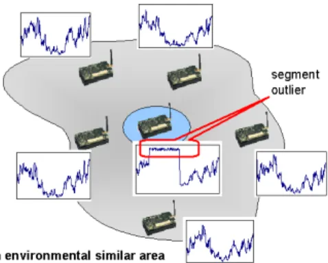
Long segmental outlier detection is based on the neigh-boring similarity measurement. We notice that envi-ronmental change is not isolated, which means any change (increasing or decreasing) will affect a close area instead of only a single point. Since sensors are always densely and redundantly deployed, nearby sen-sors will have similar patterns. Here we assume that each environmental area is monitored by several sen-sors. The idea of outlier detection is to compare a sensing series with that of its neighbors. If a sens-ing series has a similar counterpart among one of its
Figure 2: Spatially similar sensing series: sensors in the gray region are monitoring the same environmental area, and therefore have similar sensing series. The circled sensor is an outlier sensors, which can be known from its distinct sensing series.
neighbors, it is not an outlier because the probabil-ity of two failed sensors to generate similar erroneous series is very small. If a sensing series does not have any similar counterpart among its neighbors, it is higly possible to be an outlier sensor. Figure 2 plots an ex-ample of a spatially similar region, in which all the sensors should have similar sensing series. The circled sensor, which is quite different from the other sensors around it, is detected as an outlier sensor.
We use Dynamic Time Warping distance (DTW) to measure the similarity of two sensing series. The reason for not using the simpler Euclidean distance is that: (a) first, sensors in a network are loosely syn-chronized, so the sensing series are not aligned exactly; (b) second, there are different delays for different sen-sors to detect an environmental change, e.g. a fire occurs at one sensor takes a little while to spread to its neighbors. Due to the above two reasons, Euclidean distance is not suitable for measuring the similarity of sensing series.
DTW is a method that can compare two time se-ries having elastic shifting on the time axis. They are considered to be similar, although out of phase. In Figure 3, the two time series are of similar shape, but not aligned in the time axis. Euclidean distance com-pares theithpoint of one series with the ith point of
the other, and reports a dissimilar result. However, DTW distance compares the dynamic warped points as shown in the figure, and therefore can capture the similar shape of the two series. The DTW algorithm are based on dynamic programming. The classic DTW algorithm takes O(n2) time to warp two time series each with n points. This quadratic algorithm is too much for limited sensing devices. In practice, accu-rate approximation like FastDTW is installed in the sensors, which can run in linear time and space [14].
3.3 Centralized Cleaning Process
Centralized outlier cleaning is carried out after all the data are collected to the sink. Outlier cleaning is done step by step:
Figure 3: Euclidean distance and DTW distance
1. transform the sensing series to the wavelet do-main;
2. reconstruct the sensing series using the first few coefficients;
3. compare the original series with the restored series to detect outlier points;
4. use the value in the restored series to correct the outlier points;
5. compare the sensing series with that of its geo-graphically close neighbors;
6. detect an outlier sensing series if it is dissimilar with its neighboring series.
3.4 In-network Cleaning Process
The above outlier cleaning process can be moved down to the network level. It depends on the underlying data routing, so that the distributed sensors can clean the outliers during the data collection process.
3.4.1 Data Routing
In almost all techniques for in-network aggregation, a routing tree or graph based on hop count is estab-lished. Data are propagated from sensors to a sink through a minimum hop-count path [3]. This mini-mum hop-count based routing is constructed as fol-lows: The sink broadcasts an initial message to the sensor network, containing a hop count parameter. All the sensors receiving this message select the sender (now is the sink) as their parent. They then increase the hop count parameter by one, and rebroadcast the message. Finally, the message is propagated to the en-tire network, and each sensor is assigned a hop count number. During the data collection, a current hop count number is sent with the data message. By this means, the message is routed through the reversed path, which is a hop count decreasing path, to the sink as illustrated in Figure 4(a). For the sake of aggrega-tion, sensors are loosely synchronized and the data are collected hop by hop up to the sink. All the sensors with hop count number N are scheduled to transmit at a time period. Sensors with hop count number N-1 are scheduled in the next time period after the hop countN sensors have transmitted their data.
In this routing algorithm, each sensor can obtain some local topology information. Assume that sen-sor A has hopcount = N. First, A knows its direct
Figure 4: Topology of the in-network outlier cleaning
parents, the nodes who propagated the initial message with hopcount = N −1 to it. Second, A knows its siblings, who are the nodes that propagated the ini-tial message with hopcount = N. Third, A knows its direct children, the nodes from whom a data mes-sage was received withhopcount=N+ 1. The above information is obtained defaultly in the routing pro-tocol. Besides these, the sensor will actively keep a sibling list for each of its children. The child node at-taches its sibling list with the first data message sent to the parents, therefore, the sibling list for each child is known by the parent.
3.4.2 Neighboring Relation
Unlike the centralized approach, in in-network aggre-gation, each individual sensor does not know its geo-graphically nearest neighbors. The neighboring nodes considered in in-network outlier cleaning are the chil-dren, one-hop away siblings, and parents.
The parent-sibling-child relation is set up in the data routing. As illustrated in Figure 4(b), parents, children, and siblings can cover the four major direc-tions of a sensor - up, down, left, and right. We can detect a outlier sensor by comparing it with its net-work neighbors in the four directions.
3.4.3 Cleaning Process
In the outlier cleaning process, wavelet-based outlier correction is done by each sensor, and the neighboring DTW similarity is compared along the routing path of the data that goes to the sink.
At the sensor level, each sensor
1. transforms the sensing series to the wavelet do-main, and
2. selects the first few coefficients to transmit. At the network level, sensor A receives its children’s sensing series, and decides which to forward and which to delete. The outlier detection process is as follows”
1. SensorA reconstructs the children sensing series from their wavelet coefficients.
2. A calculates the DTW similarity of its children’s sensing series and itself’s.
(a) If they have similar sensing series, both A
and those similar children are flagged as
Non-outlier.
(b) If all the children series are dissimilar,A is flagged asUnknown, since other neighbors need to be compared before making an out-lier decision forA’s sensing series.
3. When A’s sensing series is transmitted to its par-ent B. For a child’s sensing series flagged as Un-known, B compares it first with the series of the siblings of this child, then with the sensing series of B itself. Remember that a sibling list for each child is maintained when the routing paths are set up.
(a) If there is a similar sensing series to that of thisUnknownchild, it is not an outlier and should be forwarded.
(b) If all the sensing series are dissimilar, this child is finally detected as an outlier after comparing with all its network neighbors. The sensing series of this child is removed from the forwarding list.
For each sensor, it’s sensing series is compared with those of its children when it receives the children’s sensing series. The comparison of siblings and parents is done by the parent sensors. In the case when a sen-sor node has multiple parents, each parent would con-duct its comparison independently. An outlier sensing series can be detected and removed by all the parents.
4
Evaluation
We have simulated a sensor network of about 900 sen-sors deployed in a grid topology. The transmission range of each sensor covers the upper, lower, left, right, upper and lower left, and upper and lower right sen-sors. The environmental sensing series of each sensor is generated from a temporal-spatial model. We have conducted simulations to evaluation our outlier clean-ing approach under several evaluation metrics.
4.1 Evaluation Dataset
The evaluation datasets are generated from a model that simulates an area with temporal-spatial corre-lated environment. A number of points called event trigger have been placed in the simulation area. The sensed value of the event trigger follows a random walk. The location of the event trigger is also a ran-dom walk on the 2D simulation area. The value of a sensor at time t is the weighted combination of the values of the event triggers, where the weight is the inverse of the normalized distance between the tar-get point and the event trigger point. Figure 5 plots a snapshot of the changing environment on a square monitoring area at a certain time. The values on the vertical axis are the current sensing readings. Finally,
Figure 5: A snapshot of a temporal-spatial correlated area
outliers are added to the dataset as random errors. An outlier may affect only one data point in the sensing series, or affect a segment lasting for a certain time pe-riod. Different amounts of outliers can be introduced, distributed randomly in the area and in time. These outliers can be of different lengths. We have adjusted the model parameters and generated several environ-mental datasets in the simulation.
4.2 Evaluation Metrics
correction ratio It measures how much the outliers are corrected in order to be closer to the real value. Given the error of the outlier value, and the er-ror of the corrected value, the correction ratio is calculated as follows:
cratio=outlier error−corrected error
outlier error
precision and recall This metric is used to mea-sure the performance of outlier detection using DTW based outlier removal. Precision is the ra-tio of the correctly detected outliers and the total number of the detected outliers. Recall is the ra-tio of the correctly detected outliers and the total number of outliers.
transmission bytes We use the total number of transmission bytes in the network to measure the reduced traffic amount. This can represent the amount of energy saved in data transmission.
4.3 Results
In this section, we will evaluate our in-network outlier cleaning approach in different scenarios. If not explic-itly specified, the default parameters listed in Figure 6 are used in the simulation.
4.3.1 Outlier Correction Ratio
We first evaluate the wavelet-based outlier correction approach when choosing different number of wavelet coefficients to represent the sensing series. We have added different amounts of outliers into the simulation scenarios - 500, 1000, 1500, and 2000 outliers. Each outlier was a single burst. The percentage of outliers
network size 30×30 the number outlier sensors 300 sensing series length 128 outlier length 10∼100 the number of wavelet
coeffi-cients 10
DTW threshold 20
Figure 6: Default parameters in the simulation. We test the change of the parameters in our evaluation.
Figure 7: Correction ratio of wavelet-based correction
in the dataset was 0.42%∼1.74%. Figure 7 plots the simulation results. The more the wavelet coefficients used, the finer the granularity. The high order wavelet coefficients can capture the outlier burst, so the cor-rection ratio keeps decreasing. On the other hand, if too few wavelet coefficients are used, the restored sens-ing series is too coarse to correct the outlier. The best correction ratio exists at 5 coefficients. Choosing 5 to 12 coefficients can give a correction ratio of over 90%. To have a good approximation of the original sensing series, we have chosen 10 coefficients in the rest of the simulations.
4.3.2 DTW Threshold
In neighboring DTW distance-based outlier removal, we have used a DTW threshold to decide whether two sensing series are similar or not. If their DTW distance is smaller than the DTW threshold, they are regarded as similar sensing series, and vice versa. We have
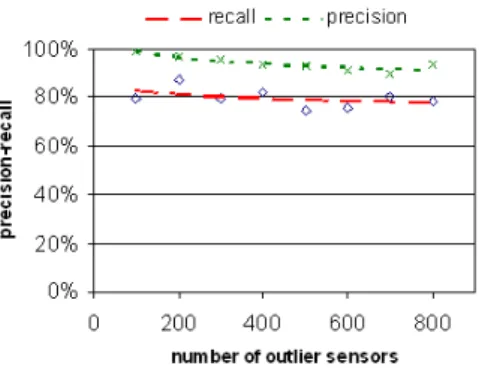
Figure 9: Recall and precision in changing outlier amount
ulated the different setting of DTW threshold and the results are shown in Figure 8. The precision of de-tecting outliers can be very high when using a thresh-old larger than 10. However, recall keeps decreasing because when the threshold is high some outliers are mistakenly counted as valid data.
4.3.3 Outlier Amount
We have also simulate different amount of outliers. As in Figure 6, the length of these outliers is randomly chosen from 10 to 100. The number of outliers in-creases from 100 to 800. We have limited each sensor to have at most one outlier. Hence, 800 outliers means 8/9 sensors suffer from failure. Figure 9 shows that both recall and precision are high. They are almost not affected by the amount of outliers.
4.3.4 Outlier Segment Length
In all the other scenarios, the length of an outlier seg-ment was randomly chosen in the region [10,100]. In this part, we have tested how the outlier length would affect outlier cleaning. We have explicitly set the out-lier length to be 10 to 100 in different runs of simu-lations, and compared their results. The simulation results are plotted in Figure 10. Precision remains high under different outlier lengths, which means our algorithm rarely reports non-outlier sensors as out-liers. However, recall is low when the outlier length is short, which means many of the true outliers are not detected. One possible reason is that the shorter outliers have already been corrected by wavelet ap-proximation. We have justified this by examining the missing outliers (undetected outliers) to see how many of them are corrected by wavelet-based outlier correc-tion. Figure 11 shows the total amount of detected and corrected outliers, where an outlier is counted as corrected if its error after correction is smaller than 1.0.
4.3.5 Traffic Reduction
Finally, we have evaluated the amount of traffic re-duction in the outlier cleaning process. Since only 10 wavelet coefficients have been used for each 128 point
Figure 10: Recall and precision in changing outlier seg-ment length
Figure 11: The total amount of corrected and removed outliers
long time series, the traffic reduction in wavelet correc-tion is about 92.19%. If an outlier is detected, the traf-fic of transmitting and forwarding this outlier is saved. Since a sensor is normally routed through a multihop path to the sink, one outlier detection will save several hops of transmission. Figure 12 shows that with the increasing number of outliers, the amount of reduced traffic in DTW-based outlier removal is also increas-ing.
5
Related Work
Outlier detection is a fundamental issue in data man-agement. Hawkins defines outlier as an observation that deviates a lot from other observations, and is
very possible to be generated from a different mech-anism [15]. Thus, outlier detection is also called de-viation detection. Most of the outlier detection tech-niques are based on data mining. Hodge and Austin classified a variety of outlier detection methods into three categories in their survey paper [16]: Unsuper-vised clustering based on distance and density, which determines the outliers with no prior knowledge of the data [17]; supervised classification that required pre-labelled data and a machine learning process [18]; and
semi-supervised methods that can tune the detection model incrementally as new data arrive [19]. Most of the proposed outlier detection approaches are central-ized and off-line. They cannot be applied to sensor network applications directly.
Only a few papers have tried to address in-network outlier detection in the context of sensor networks. Palpanaset al. have proposed an in-network approach for distributed online deviation detection for stream-ing data [20]. However, this approach highly depends on the existence of high capacity sensors to manage groups of other sensors and perform outlier detection. Another related work proposed by Branchet al. uses a non-parametric, unsupervised method to detect out-liers. They also use the distance-based metrics in the detection [21]. Hida et al. proposed a method to perform outlier detection in query processing (such as Max and Avg), so that query aggregation can be more reliable [22]. These approaches do not combine the temporal spatial similarity in outlier detection, be-cause they detect outliers as a single value. However, in this paper we try to detect outliers in a number of time series. As a first step, we use wavelet based outlier correction and DTW distance-based outlier re-moval, which can be thought of as a distance based approach. This requires that the data in the whole area exhibit the same distribution, and the user should have some knowledge of the data to set an appropriate threshold. Our future work tries to address the outlier problem when the data are of different distribution. In this case, a single threshold may not be appropriate, and a sophisticated statistical model is required [23].
6
Conclusions
In this paper, we have presented an in-network out-lier cleaning approach for sensor network data collec-tion applicacollec-tions, using wavelet based outlier correc-tion and DTW distance-based outlier removal. We have considered the spatial-temporal correction of en-vironmental data; we not only detected but also tried to correct the outliers; we were able to remove the outliers within 2 network forwarding hops and reduce a large amount of the traffic. We have evaluated our approach under comprehensive simulations.
References
[1] S. Shekhar, C. T. Lu, and P. Zhang, “Detecting graph-based spatial outliers: Algorithms and applications,” in
SIGKDD, 2001.
[2] Berndt and Clifford, “Using dynamic time warping to find patterns in time series,” inKDD Workshop, 1994. [3] J. Al-Karaki and A. Kamal, “Routing techniques in wireless
sensor networks: a survey,”IEEE Wireless Comm., no. 4, pp. 6–28, 2004.
[4] G. Pottie and W. Kaiser, “Wireless integrated network sensors,” Communications of the ACM, vol. 43, no. 5, p. 51C58, 2000.
[5] A. Mainwaring, J. Polastre, R. Szewczyk, and D. Culler, “Wireless sensor networks for habitat monitoring,” Intel Research, Tech. Rep. IRB-TR-02-006, Jun. 2002.
[6] R. Cardell-Oliver, K. Smettem, M. Kranz, and K. Mayer, “A reactive soil moisture sensor network: Design and field evaluation,” International Journal of Distributed Sensor Networks, vol. 1, 2005.
[7] L. M. Ni, Y. Liu, Y. C. Lau, and A. Patil, “Landmarc: Indoor location sensing using active rfid,” ACM Wireless Networks, vol. 10, no. 6, pp. 701–710, November 2004. [8] S. Madden, M. Franklin, J. Hellerstein, and W. Hong, “Tag:
a tiny aggregation service for ad-hoc sensor networks,” in
OSDI, 2002.
[9] M. A. Sharaf, J. Beaver, A. Labrinidis, and P. K. Chrysan-this, “Balancing energy efficiency and quality of aggregate data in sensor networks,” inVLDB, 2004.
[10] A. Manjhi, S. Nath, and P. B. Gibbons, “Tributaries and deltas: Efficient and robust aggregation in sensor network streams,” inSIGMOD, Baltimore, Maryland, USA, 2005. [11] J. Considine, F. Li, G. Kollios, and J. Byers, “Approximate
aggregation techniques for sensor databases,” in ICDE, Boston, Massachusetts, USA, 2004.
[12] W. Xue, Q. Luo, L. Chen, and Y. Liu, “Contour map matching for event detection in sensor networks,” in SIG-MOD, 2006.
[13] D. Nychka, W. Piegorsch, and L. Cox, Case Studies in Environmental Statistics. Springer, New York, 1998. [14] S. Salvador and P. Chan, “Fastdtw: Toward accurate
dy-namic time warping in linear time and space,” in KDD Workshop, 2004.
[15] D. Hawkins,Identification of Outliers. Chapman and Hall, 1980.
[16] V. Hodge and J. Austin, “A survey of outlier detec-tion methodologies,”Artificial Intelligence Review, vol. 22, no. 2, pp. 85–126, October 2004.
[17] Rousseeuw and A. Leroy, Robust Regression and Outlier Detection, 3rd ed. J. Wiley, New York, 1996.
[18] G. Williams, R. Baxter, H. He, S. Hawkins, and Lifang.Gu, “A comparative study of rnn for outlier detection in data mining,” inICDM, 2002.
[19] D. Zhang, D. Gatica-Perez, S. Bengio, and I. McCowan, “Semi-supervised adapted hmms for unusual event detec-tion,” inCVPR, 2005.
[20] T. Palpanas, D. Papadopoulos, V. Kalogeraki, and D. Gunopulos, “Distributed deviation detection in sensor networks,”ACM SIGMOD, vol. 32, no. 4, pp. 77–82, Oc-tober 2003.
[21] J. W. Branch, B. K. Szymanski, C. Giannella, R. Wolff, and H. Kargupta, “In-network outlier detection in wireless sensor networks,” inICDCS, 2006.
[22] Y. Hida, P. Huang, and R. Nishtala, “Aggregation query under uncertainty in sensor networks,” Department of Elec-trical Engineering and Computer Science. University of California, Berkeley, Tech. Rep., 2004.
[23] S. Subramaniam, T. Palpanas, D. Papadopoulos, V. Kalogeraki, and D. Gunopulos, “Online outlier detection in sensor data using non-parametric models,” in