A Python package for Bayesian estimation using Markov Chain Monte Carlo

(1)

Strickland, C. M., Denham, R. J.,Alston, C. L., &Mengersen, K. L.(2011) PyMCMC : a Python package for Bayesian Estimation using Markov chain Monte Carlo. .

This file was downloaded from: http://eprints.qut.edu.au/43469/

c

Notice: Changes introduced as a result of publishing processes such as copy-editing and formatting may not be reflected in this document. For a definitive version of this work, please refer to the published source:

(2)

Estimation Using Markov Chain Monte Carlo

C. M. Strickland Queensland University of Technology R. J. Denham Department of Environment and Resource Management C. L. Alston Queensland University of Technology K. L. Mengersen Queensland University of Technology Abstract

Markov chain Monte Carlo (MCMC) estimation provides a solution to the complex integration problems that are faced in the Bayesian analysis of statistical problems. The implementation of MCMC algorithms is, however, code intensive and time consuming. We have developed aPythonpackage, which is calledPyMCMC, that aids in the construction of MCMC samplers and helps to substantially reduce the likelihood of coding error, as well as aid in the minimisation of repetitive code. PyMCMC contains classes for Gibbs, Metropolis Hastings, independent Metropolis Hastings, random walk Metropolis Hastings, orientational bias Monte Carlo and slice samplers as well as specific modules for common models such as a module for Bayesian regression analysis. PyMCMCis straightforward to optimise, taking advantage of thePythonlibraries NumpyandScipy, as well as being readily extensible withCorFortran.

Keywords: MCMC, Metropolis Hastings, Gibbs, Bayesian, OBMC, slice sampler,Python.

1. Introduction

The most common approach currently used in the estimation of Bayesian Models is Markov chain Monte Carlo (MCMC).PyMCMCis aPython module that is designed to simplify the construction of Markov chain Monte Carlo (MCMC) samplers, without sacrificing flexibility or performance. Python has extensive scientific libraries, is easily extensible, has a clean syntax and powerful programming constructs, making it an ideal programming language to build an MCMC library; see van Rossum (1995) for further details on the programming language Python. PyMCMC contains objects for the Gibbs sampler, Metropolis Hastings (MH), independent MH, random walk MH, orientational bias Monte Carlo (OBMC) as well as the slice sampler: see for exampleRobert and Casella(1999) for details on standard MCMC algorithms. The user can simply piece together the algorithms required and can easily include their own modules, where necessary. Along with the standard algorithms,PyMCMCincludes a module for Bayesian regression analysis. This module can be used for the direct analysis of linear models, or as a part of an MCMC scheme, where the conditional posterior has the form of a linear model. It also contains a class that can be used along with the Gibbs sampler for Bayesian variable selection.

The flexibility of PyMCMC is important in practice, as MCMC algorithms usually need to be tailored to the problem of interest in order to ensure good results. Issues such as block

(3)

size and parameterisation can have a dramatic effect on the convergence of MCMC sampling schemes. For instance, Lui, Wong, and Kong (1994) show theoretically that jointly sampling parameters in a Gibbs scheme typically leads to a reduction in correlation in the associated Markov chain in comparison to individually sampling parameters. This is demonstrated in practical applications in Carter and Kohn (1994) and Kim, Shephard, and Chib (1998). Reducing the correlation in the Markov chain enables it to move more freely through the parameter space and as such enables it to escape from local modes in the posterior distribution. Parameterisation can also have a dramatic effect on the convergence of MCMC samplers; see for example Gelfand, Sahu, and Carlin(1995), Sahu and Roberts(1997), Pitt and Shephard (1999), Robert and Mengersen (1999), Fr¨uwirth-Schnatter (2004) and Strickland, Martin, and Forbes(2008), who show that the performance of the sampling schemes can be improved dramatically with the use of efficient parameterisation.

PyMCMCaims to remove unnecessary repetitive coding and hence reduce the chance of cod-ing error, and importantly, greatly speed up the construction of efficient MCMC samplers. This is achieved by taking advantage of the flexibility of Python, which allows for the imple-mentation of very general code. Another feature of Python, which is particularly important, is it is also extremely easy to include modules from compiled languages such as CandFortran. This is important to many practitioners who are forced, by the size and complexity of their problems, to write their MCMC programs entirely in compiled languages, such asC/C++and Fortranin order to obtain the necessary speed for feasible practical analysis. WithPython, the user can simply compile Fortran code using a module called F2py(Peterson 2009), or inline C using Weave, which is a part of Scipy (Oliphant 2007), and use the subroutines directly from Python. F2pycan also be used to directly call C routines with the aid of a Fortran sig-nature file. This enables the use ofPyMCMCandPythonas a rapid application development environment, without compromising on performance by requiring only very small segments of code written in a compiled language. It should be mentioned that for most reasonable sized problems PyMCMCis sufficiently fast for practical MCMC analysis without the need for specialised modules.

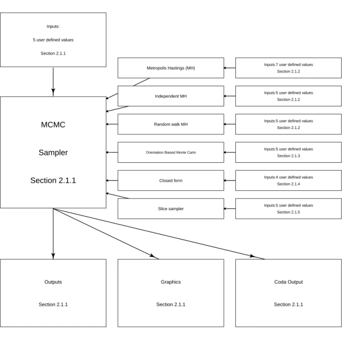
Figure 1 is a flow chart that depicts the structure of PyMCMC. Essentially, the implemen-tation of an MCMC sampler can be seen to centred around the class MCMC, which acts as a container for various algorithms that are used in sampling from the conditional posterior distributions that make up the MCMC sampling scheme.

The structure of the paper is as follows. In Section2 the algorithms contained inPyMCMC

and the user interface are described. This includes the Gibbs sampler, the Metropolis based algorithms and the slice sampler. Section 2 also contains a description of the Bayesian re-gression module. Section 3 contains three empirical examples that demonstrate how to use

PyMCMC. The first example demonstrates how to use the regression module for the Bayesian analysis of the linear model. In particular, the stochastic search variable selection algorithm, see George and McCulloch (1993) and Marin and Robert (2007), is used to select a set of ‘most likely models’. The second example demonstrates how to use PyMCMCto analyse the loglinear model and the third example demonstrates how to usePyMCMCto analyse a linear model with first order autoregressive errors. Section 4 contains discussion on the efficient implementation of the MCMC algorithms using PyMCMC. Section 5 describes how to use

(4)

Inputs:

5 user defined values

Section 2.1.1

MCMC

Sampler

Section 2.1.1

Metropolis Hastings (MH) Inputs:7 user defined values

Section 2.1.2

Independent MH Inputs:5 user defined values

Section 2.1.2

Random walk MH Inputs:5 user defined values

Section 2.1.2

Orientation Biased Monte Carlo Inputs:5 user defined values Section 2.1.3

Closed form Inputs:4 user defined values

Section 2.1.4

Slice sampler Inputs:5 user defined values

Section 2.1.5 Outputs Section 2.1.1 Graphics Section 2.1.1 Coda Output Section 2.1.1

Figure 1: Flow chart illustrating the implementation ofPyMCMC.

2. Bayesian analysis

Bayesian analysis quantifies information about the unknown parameter vector of interest,θ,

(5)

which is defined such that

p(θ|y)∝p(y|θ)×p(θ), (1) where p(y|θ) denotes the pdf ofygiven θ andp(θ) is the prior pdf forθ.The most common approach used for inference about θ is MCMC.

2.1. Markov chain Monte Carlo methods and implementation

In the following subsections, a brief description of each algorithm and the associated pro-gramming interface is included.

Markov chain Monte Carlo sampling

If we partition θ into sblocks, that is θ = (θ1,θ2, . . . ,θs)T, then thejth step for a generic MCMC sampling scheme is given by:

Algorithm 1Gibbs sampler 1. Sampleθj₁ from pθ1|y, θj −1 2 ,θ j−1 3 , . . . ,θj −1 s , 2. Sample θj₂ from pθ2|y, θ1j,θ j−1 3 ,θ j−1 4 , . . . ,θsj−1 , .. . s. Sample θ_sj frompθs|y, θj1,θ j 2, . . . ,θ j s−1 .

An important special case of Algorithm1 is the Gibbs sampler, which is an algorithm that is proposed in Gelfand and Smith (1990). Specifically, when each of θ1,θ2, . . . ,θs, is sampled from a closed form then this algorithm corresponds to that of the Gibbs sampler. PyMCMC

contains a class that facilitates the implementation of Algorithm 1, in which the user must define functions to sample from each block, i.e.,. a function for each of θi, for i = 1, . . . , s. These functions may be defined using the Metropolis based or slice sampling algorithms that are part ofPyMCMC. The class is namedMCMC and the following arguments are required in the initialisation of the class:

nit: The number of iterations.

burn: The burnin length of the MCMC sampler.

data: A dictionary (Python data structure) containing any data, functions or objects that the user would like to have access to when defining the functions that are called from the Gibbs sampler.

blocks: A list (Pythondata structure) containing functions that are used to sample from the full conditional posterior distributions of interest.

(6)

loglike A tuple (a Python data structure) containing a function that evaluates the log-likelihood, number of parameters and the name of the dataset. For example:

loglike = (loglike, nparam, ‘yvec’). If this is defined then the log-likelihood and the BIC will be reported in the standard output.

transform A dictionary, where the keys are the names of the parameters and the asso-ciated values are functions that transform the iterates stored in the MCMC scheme. This can be useful when the MCMC algorithm is defined under a particular pa-rameterisation, but where it is desirable to report the results under a different parameterisation.

Several functions are included as a part of the class:

sampler()- Used to run the MCMC sampler.

get_mean_cov(listname) - Returns the posterior covariance matrix for the parameters named in listname, where listname is a list that contains the parameter names of interest.

get_parameter(name)- Returns the iterates for the named parameter including the burnin.

get_parameter_exburn(name) - Returns the iterates for the named parameter excluding the burnin.

get_mean_var(name) - Returns the estimate from the MCMC estimation for the posterior mean and variance for the parameter defined by name.

set_number_decimals(num)- Sets the number of decimal places for the output.

output(**kwargs)- Used to produce output from the MCMC algorithm.

**kwargs- Optional arguments that control the output.

parameters: A dictionary, list or string specifying the parameters that are going to be presented.

• If a string is passed (e.g.,: parameters = ‘beta’), all elements of that parameter are given.

• If a list (e.g.,: parameters = [‘alpha’, ‘beta’]), all elements of each parameter in the list are given.

• If a dictionary (e.g.,: parameters = {‘alpha’:{‘range’:range(5)}}), then there is the possibility to add an additional argument ‘range’ that tells the output to only print a subset of the parameters. The above example will print information for alpha[0], alpha[1],..., alpha[4]

only.

custom- A user defined function that produces custom output.

filename- A filename to which the output is printed. By default output will be printed to stdout.

plot(blockname, **kwargs) - Create summary plots of the MCMC sampler. By default, a plot of the marginal posterior density, an ACF plot and a trace plot are produced for each parameter in the block. The plotting page is divided into

(7)

a number of subfigures. By default, the number of columns are approximately equal to the square root of the total number of subfigures divided by the number of different plot types. Arguments toplot are:

blockname - The name of the parameter, for which summary plots are to be generated.

**kwargs- An optional dictionary (Pythondata structure) containing information to control the summary plots. The available keys are summarised below:

elements: A list of integers specifying the elements that will be plotted. For example, if the blockname is‘beta’ andβ= (β0, β1. . . βn) then you may specify elements aselements = [0,2,5].

plottypes: A list giving the type of plot for each parameter. By default the plots are‘density’,‘acf’and‘trace’. A single string is also acceptable.

filename: A string providing the name of an output file for the plot. As a plot of a block may be made up of a number of subfigures, the output name will be modified to give a separate filename for each subfigure. For example, if the filename is passed as ‘plot.png’, and there are multi-ple pages of output, it will produce the filesplot001.png,plot002.png, etc. The type of file is determined by the extension of the filename, but the output format will also depend on the plotting backend being used. If the filename does not have a suffix, a default format will be chosen based on the graphics backend. Most backends support png, pdf, ps, eps and svg (see the documentation for Matplotlib for further details http://matplotlib.sourceforge.net).

individual: A Boolean option. If true, then each subplot will be done on an individual page.

rows: Integer specifying the number of rows of subfigures on a plotting page.

cols: Integer specifying the number of columns of subfigures on a plotting page.

CODAoutput(**kwargs)- Output the results in a format suitable for reading in with the statistical package Convergence Diagnostic and Output Analysis (CODA) (Plum-mer, Best, Cowles, and Vines 2006). By default, there will be two files created,

coda.txtand coda.ind.

**kwargs- An optional dictionary controlling theCODAoutput.

filename: A string to provide an alternative filename for the output. If the file has an extension this will form the basis for the data file and the index file will be named by replacing the extension with ind. If no extension is in the filename then two files will be created and named by adding the extensions .txtand .ind to the given filename.

parameters: A string, a list or a dictionary that specify the items writ-ten to file. It can be a string such as ‘alpha’ or it can be a list (e.g.,

[‘alpha’,‘beta’]) or it can be a dictionary (e.g.,

{‘alpha’:{‘range’:[0,1,5]}}. If you supply a dictionary the key is the parameter name. It is also permissible to have a range key with a range of elements. If the range isn’t supplied it is assumed that the user wants all of the elements.

(8)

thin: Integer specifying how to thin the output. For examples ifthin = 10, then every tenth element will be written to theCODAoutput.

Metropolis Hastings

A particularly useful algorithm that is often used as a part of MCMC samplers is the MH algorithm (Algorithm2); see for exampleRobert and Casella(1999). This algorithm is usually required when we cannot easily sample directly from p(θ|y), however, we have a candidate density q(θ|y,θj−1), which in practice is close to p(θ|y), and is more readily able to be sampled. The MH algorithm at the jth iteration forj= 1,2, . . . , M is given by the following steps:

Algorithm 2Metropolis Hastings

1. Draw a candidateθ∗ from the densityq θ|y,θj−1

,

2. Acceptθj =θ∗ with probability equal to min 1,_pp₍_θ(θj−∗|1y_|_y)₎/ q(θ∗|y,θj−1₎ q(θj−1_|_y_,_θ∗₎ , 3. Otherwiseθj =θj−1.

PyMCMCincludes a class for the MH algorithm, which is called MH. To initialise the class the user needs to define:

func- User defined function that returns a sample for the parameter of interest.

actualprob - User defined function that returns the log probability of the parameters of interest evaluated using the target density.

probcandprev- User defined function that returns the log ofq θ∗|y,θj−1

.

probprevcand- User defined function that returns the log ofq θj−1|y,θ∗

.

init_theta- Initial value for the parameters of interest.

name- The name of the parameter of interest.

**kwargs- Optional arguments:

store

‘all’(default), stores every iterate for the parameter of interest. This is required for certain calculations.

‘none’, does not store any of the iterates from the parameter of interest.

fixed_parameter- Is used if the user wants to fix the parameter value that is returned. This is used for testing MCMC sampling schemes. This command will override any other functionality.

(9)

Independent Metropolis Hastings

The independent MH is a special case of the MH described in Algorithm 2. Specifically, the independent MH algorithm is applicable when we have a candidate density q(θ|y) =

q(θ|y,θj−1). The independent MH algorithm at the jth iteration for j= 1,2, . . . , M is given by Algorithm3.

Algorithm 3Independent MH algorithm

1. Draw a candidateθ∗ from the densityq(θ|y),

2. Acceptθj ₌_θ∗ _{with probability equal to min}n₁_, p(θ∗|y) p(θj−1_|_y₎/ q(θ∗|y) q(θj−1_|_y₎ o , 3. Otherwise acceptθj =θj−1.

PyMCMCcontains a class for the independent MH algorithm, namedIndMH. To initialise the class the user needs to define:

func- A user defined function that returns a sample for the parameter of interest.

actualprob- A user defined function that returns the log probability of the parameters of interest evaluated using the target density.

candpqrob - A user defined function that returns the log probability of the parameters of interest evaluated using the candidate density.

init_theta- Initial value for the parameters of interest.

name- Name of the parameter of interest.

store

Random walk Metropolis Hastings

A useful and simple way to construct an MH candidate distribution is via

θ∗ =θj−1+ε, (2) where ε is a random disturbance vector. If ε has a distribution that is symmetric about zero then the MH algorithm has a specific form that is referred to as the random walk MH algorithm. In this case, note that the candidate density is both independent ofyand, due to

(10)

symmetry, q θ∗|θj−1

=q θj−1|θ∗

. The random walk MH algorithm at the jth iteration forj= 1,2, . . . , M is given by Algorithm 4.

Algorithm 4Random Walk MH

1. Draw a candidateθ∗from Equation2where the random disturbanceεhas a distribution symmetric about zero.

2. Acceptθj =θ∗ with probability equal to minn1,_p₍p_θ(θj−∗|1y_|_y)₎

o , 3. Otherwise acceptθj =θj−1.

A typical choice for the distribution ofεis a Normal distribution, that isε∼i.i.d.N(0,Ω) where the covariance matrix Ωis viewed as a tuning parameter. PyMCMCincludes a class for the random walk MH algorithm, named RWMH. The class RWMH is defined assuming ε follows a normal distribution. Note that more general random walk MH algorithms could be constructed using the MH class. To initialise the class the user must specify:

post - A user defined function for the log of full conditional posterior distribution for the parameters of interest.

csig- Scale parameter for the random walk MH algorithm.

init_theta- Initial value for the parameter of interest.

name- Name of the parameter of interest.

store

adaptive-‘GFS’, Then the adaptive random walk MH algorithm ofGarthwaite, Fan, and Scisson (2010) will be used to optimiseΩ.

Orientational bias Monte Carlo

The multiple try Metropolis (Liang, Lui, and Wong 2000) generalises the MH algorithm to allow for multiple proposals. The OBMC algorithm is a special case of the multiple try Metropolis that is applicable when he candidate density is symmetric. The OBMC Algorithm at iterationj is as follows:

(11)

Algorithm 5Orientational Bias Monte Carlo

1. Draw L candidates θ_l∗, l = 1,2, . . . , L, independently from the density q θ|y,θj−1 , where q θ|y,θj−1

is a symmetric function.

2. Construct a probability mass function (pmf ) by assigning to each θ_l∗, a probability proportional top(θ_l∗|y).

3. Selectθ∗∗ randomly from this discrete distribution.

4. DrawL−1 reference pointsrl, l= 1,2, . . . , L−1, independently fromq(θ|y,θ∗∗) and set rL=θj−1.

5. Acceptθj =θ∗∗ with probability equal to min 1, PL l=1p(θ ∗ l|y) PL l=1p(rl|y) , 6. Otherwise acceptθj ₌_θj−1_.

PyMCMCimplements a special case of the OBMC algorithm, for which the candidate density is multivariate normal, making it a generalisation of the random walk MH algorithm. The class for the OBMC algorithm is namedOBMC. To initialise the class the user must specify:

post - A user defined function for the log of the full conditional posterior distribution for the parameters of interest.

ntry- Number of candidates, L.

csig- A scale parameter for the OBMC algorithm.

init_theta- Initial value for the parameter of interest.

store

Closed form sampler

A class is included so that the user can specify a function to sample the parameters of interest when there is a closed form solution. The name of the class is CFsampler. To initialise the class the user must specify:

(12)

init_theta- Initial value for the unknown parameter of interest.

name- The name of the parameter of interest.

**kwargs- Optional parameters:

store

Slice sampler

The slice sampler is useful for drawing values from complex densities; see Neal (2003) for further details. The required distribution must be proportional to one or a multiple of several other functions of the variable of interest;

p(θ)∝f1(θ)f2(θ)· · ·fn(θ).

A set of values from the distribution is obtained by iteratively sampling a new value,ω, from the vertical slice between 0 and fi(θ), then sampling a value for the parameter θ from the horizontalslicethat consists of the set of possible values ofθ, for which the previously sampled

ω≤p(θ). This leads to the slice sampler algorithm, which can be defined at iterationj using Algorithm6.

Algorithm 6Slice sampler

1. Fori= 1,2, . . . , n, drawωi∼Unif[0, fi(θj−1)].

2. Sampleθj ∼Unif[A] whereA={θ:f1(θ)≥ω1 ∈f2(θ)≥ω2 ∈ · · · ∈fn(θ)≥ωn}.

In cases where the density of interest is not unimodal, determining the exact set A is not necessarily straightforward. The stepping out algorithm ofNeal (2003) is used to obtain the set A. This algorithm is applied to each of the n slices to obtain the joint maximum and minimum of the slice. This results in a sampling interval that is designed to draw a new θj in the neighbourhood of θj−1 and may include values outside the permissible range of A. The user is required to define an estimated typical slice size (ss), which is the width of set A, along with an integer value (N), which limits the width of any slice toN×ss. The stepping out algorithm (7) is:

(13)

Algorithm 7Stepping out

1. Initiate lower (LB) and upper (UB) bounds for slice defined by setA.

• U ∼Unif(0,1); – LB=θj−1−ss×U, – U B =LB+ss. 1. SampleV ∼Unif(0,1). 2. SetJ = Floor(N×V). 3. SetZ= (N −1)−J.

4. Repeat whileJ >0 andωi < fi(LB)∀i;

• LB = LB - ss,

• J =J−1.

5. Repeat whileZ >0 and ωi < fi(U B)∀i;

• UB = UB + ss,

• Z = Z - 1.

6. Sampleθj ∼Unif(LB, U B).

The value of θj is accepted if it is drawn from a range (LB, U B) ∈ A. If it is outside the allowable range due to the interval (LB, U B) being larger in range than the set A we then invoke a shrinkage technique to resample θj and improve the sampling efficiency of future draws, until an acceptable θj is drawn. The shrinkage algorithm is implemented as follows, repeating this algorithm until exit conditions are met.

Algorithm 8Shrinkage 1. U ∼Unif(0,1).

2. θj ₌_LB₊_U_×₍_{U B}₋_LB_);

• If ωi < fi(ωi)∀i, acceptθj and exit,

• Else if θj < θj−1, setLB=θj and return to step 1,

• Else set U B=θj and return to step 1.

PyMCMCincludes a class for the slice sampler namedSliceSampler. To initialise the class the user must define:

(14)

init_theta- An initial value forθ.

ssize- A user defined value for the typical slice size.

sN- An integer limiting slice size toN ×ss.

store

2.2. Normal linear Bayesian regression model

Many interesting models are partly linear for a subset of the unknown parameters. As such drawing from the full conditional posterior distribution for the associated parameters may be equivalent to sampling the unknown parameters in a standard linear regression model.

PyMCMC includes several classes that aid in the analysis of linear or partly linear mod-els. In particular the classesLinearModel,CondRegressionSampler,CondScaleSamplerand

StochasticSearch are useful for this purpose. These classes are described in this section. For the standard linear regression model (seeZellner(1971), assume the (n×1) observational vector,y,is generated according to

y=Xβ+ε; ε∼N(0, σ2I), (3)

whereX is an (n×k) matrix of regressors,β is a (k×1) vector of regression coefficients and εis a normally distributed random variable with a mean vector0 and an (n×n) covariance matrix, σ2I. Assuming that both β and σ are unknown then the posterior distribution for Equation3 is given by p(β, σ|y,X)∝p(y|X,β, σ)×p(β, σ), (4) where p(y|X,β, σ)∝σ−nexp − 1 2σ2(y−Xβ) T_(y₋_Xβ)_, ₍₅₎

is the jointpdf forygivenX,β andσ, and p(β, σ) denotes the joint priorpdf forβ and σ. A class namedLinearModelis defined to sample from the posterior distribution in Equation4. One of four alternative priors may be used in the specification of the model. The default choice is Jeffreys prior. Denoting the full set of unknown parameters asθ = (βT, σ)T,then Jeffreys prior is defined such that

(15)

whereI(θ) is the Fisher information matrix for θ.For the normal linear regression model in 3, given the assumption thatβ andσ area priori independent, Jeffreys prior is flat over the real number line for β, and σ is distributed such that

p(σ)∝ 1

σ. (7)

See Zellner (1971) for further details on Jeffreys prior. Three alternative informative prior specifications are allowed, namely the normal-gamma, the normal-inverted-gamma and Zell-ner’s g-prior; seeZellner(1971) andMarin and Robert(2007) for further details. The normal-gamma prior is specified such that

β|κ∼N(β,V−1), κ∼G _ν 2, S 2 , (8)

whereκ=σ−2andβ,V, νandSare prior hyperparameters that take user defined values. For the Normal-gamma prior,LinearModelproduces estimates forκ,βTT _{rather than}_σ,_βT . The Normal-inverted gamma prior is specified such that

β|σ−2 ∼N(β,V−1), σ−2∼IG _ν 2, S 2 , (9)

whereβ, V, ν and S are prior hyperparameters, which take values that are set by the user. Zellner’s g-prior is specified such that

β|σ ∼N

β, gσ2XTX−1

, p(σ)∝σ−1, (10) whereβ and g are hyperparameters with values that are specified by the user. To initialise the classLinearModel the user must specify:

yvec- One dimensional Numpyarray containing the data.

xmat- Two dimensional Numpyarray contain the regressors.

prior- A list containing the name of the prior and the corresponding hyperparameters. Examples:

prior = [‘normal_gamma’, betaubar, Vubar, nuubar, Subar] ,

prior = [‘normal_inverted_gamma’,betaubar, Vubar, nuubar, Subar] and

prior = [‘g_prior’, betaubar, g].

If none of these options are chosen or they are miss-specified then the default prior will be Jeffreys prior.

LinearModel contains several functions that may be of interest to the user. In particular:

sample()- Returns a sample ofσandβfrom the joint posterior distribution for the normal-inverted gamma prior, Jeffreys prior and Zellner’s g-prior. If the normal-gamma prior is specified then sample()returnsκ and β.

(16)

update_yvec(yvec)- Updates yvec in LinearModel. This is often useful when the class is being used as a part of the MCMC sampling scheme.

update_xmat(xmat)- Updates xmat inLinearModel. This is often useful when the class is being used as a part of the MCMC sampling scheme.

loglike(scale, beta)- Returns the log-likelihood.

posterior_mean() - Returns the posterior mean for the scale parameter (either σ or κ

depending on the specified prior) and β.

get_posterior_covmat()- Returns the posterior covariance matrix forβ.

bic()- Returns the Bayesian information criterion; see Kass and Raftery(1995) for details.

plot(**kwargs) - Produces standard plots. Specifically the marginal posterior density in-tervals for each element of βand for the scale parameter (σ orκ).

residuals - Returns the residual vector from the regression analysis. The residuals are calculated with β evaluated at the marginal posterior mean.

output - Produces standard output for the regression analysis. This includes the means, standard deviations and highest posterior density (HPD) intervals for the marginal posterior densities for each element of β and for the scale parameter (σ or κ). The output also reports the log-likelihood and the BIC.

In MCMC sampling schemes it is common that for a subset of the unknown parameters of interest the full conditional posterior distribution will correspond to that of a linear regression model, where the scale parameter is known. For the linear regression model specified in Equation 3 the posterior distribution for the case thatσ is known is as follows

p(β|y,X,β, σ)∝p(y|X,β, σ)×p(β), (11) wherep(y|X,β, σ) is described in Equation5andp(β) is the priorpdf forβ.To sample from Equation 11 a class named CondRegressionSamplercan be used. The user may specify one of three alternative priors. The default prior is Jeffreys prior, which for β is simply a flat prior over the real number line. A normally distributed prior forβis another option, and can be specified such that

β∼Nβ,V−1.

The user may also specify theira priori beliefs using Zellner’s g-prior, where β|σ ∼Nβ, gσ2XTX.

To initialise the class the user must specify:

yvec- A one dimensional Numpyarray containing the data.

xmat- A two dimensional Numpyarray containing the regressors.

(17)

prior- A list containing the name of the prior and the corresponding hyperparameters. Examples:

prior=[‘normal’, betaubar, Vubar] or [‘g_prior’, betaubar, g].

If none of these options are chosen or they are miss-specified then the default prior will be Jeffreys prior.

CondRegressionSampler contains several functions that may be of interest to the user. In particular:

sample(sigma) - Returns a sample ofβ from the posterior distribution specified in 11.

get_marginal_posterior_mean()- Returns the marginal posterior mean for11.

get_marginal_posterior_precision()- Returns the marginal posterior precision for the linear conditional posterior distribution specified in 11.

update_yvec(yvec)- Updates yvec inCondRegressionSampler. This is often useful when the class is being used as a part of an MCMC sampling scheme.

update_xmat(xmat)- Updates xmat in CondRegressionSampler. This is often useful when the class is being used as a part of an MCMC sampling scheme.

Many Bayesian models contain linear components with unknown scale parameters, hence a class has been specified namedCondScaleSampler, which can be used to individually sample scale parameters from their posterior distributions. In particular, we wish to sample from

p(σ|y,θ), (12)

where θ is the set of unknown parameters of interest excluding σ. The user may choose to use one of three priors. The Jeffreys prior, which forσ given the posterior in Equation 12 is as follows

p(σ)∝ 1 σ.

The second option is to specify an inverted-gamma prior, such that

σ ∼IG _ν 2, S 2 .

Alternatively, the user may specify a gamma prior forκ= _σ12,where

κ∼G _ν 2, S 2 .

To initialise the classCondScaleSamper the user may first specify:

**kwargs- Options arguments:

prior- List containing the name of the prior and the corresponding hyperparameters. Examples:

prior=[‘gamma’,nuubar,subar] or

prior=[‘inverted-gamma’, nuubar, subar]. If no prior is specified the Jeffreys prior is used.

(18)

PyMCMCalso includes another class that can be used for the direct analysis of the linear regression model. The class is calledStochasticSearchand can be used in conjunction with the classMCMC, for the purpose of variable selection.

The stochastic search algorithm can be used for variable selection in the linear regression model. Given a set ofkpossible regressors there are 2k_{models to choose from. The stochastic} search algorithm, as proposed byGeorge and McCulloch (1993), uses the Gibbs sampler to select a set of ‘most likely’ models. The stochastic search algorithm is implemented in the classStochasticSearch. The specific implementation followsMarin and Robert(2007). The algorithm introduces the vectorγ,which is used to select the explanatory variables that are to be included in the model. In particular,γis defined to be a binary vector of orderk, whereby the inclusion of theithregressor implies that theithelement ofγ is a one, whilst the exclusion of theith regressor implies that theithelement is zero. It is assumed that the first element of the design matrix is always included and should typically be a column of ones which is used to represent the constant or intercept in the regression. The algorithm specified to sampleγ is a single move Gibbs sampling scheme; for further details seeMarin and Robert(2007). To use the class StochasticSearch the user must specify their a priori beliefs that the unknown parameters of interest, (σ,βT)T,are distributed following Zellner’s g-prior, which is described in Equation10. StochasticSearch is designed to be used in conjunction with the MCMC sampling class. To initialiseStochasticSearch the user must specify:

yvec- One dimensional Numpyarray containing the dependent variable.

xmat- Two dimensional Numpyarray containing the regressors.

prior- List with the following structure[betaubar, g].

The classStochasticSearch also contains the following function:

sample_gamma(store)- Returns a sample ofγ.The only argument to pass into the function

sample_gamma is the storage dictionary that is passed by default to each of the classes that are called from the class MCMC inPyMCMC.

3. Empirical illustrations

PyMCMC is illustrated though three examples. Specifically, a linear regression example with variable selection, a log-linear example and a linear regression model with first order autoregressive errors. For each example, the model of interest is specified, then the code used for estimation is shown, following which a brief description of code is given. Each example uses the module forPyMCMC, along with thePythonlibrariesNumpy,ScipyandMatplotlib: see Oliphant (2007); Hunter (2007) for further details of these Python libraries. Example 3 further uses the libraryPysparse(Geus 2011).

3.1. Example 1: Linear regression model: Variable selection and estimation The data used in this example are a response of crop yield modelled using various chemical measurements from the soil. As the results of the chemical analysis of soil cores are done in a

(19)

laboratory, many input variables are available and the data analyst would like to determine the variables that are most appropriate to use in the model.

The normal linear regression model in Equation3is used for the analysis. To select the set of ‘most probable’ regressors we use the stochastic search variable selection approach described in Section2.2using a subset of 19 explanatory variables.

In addition to PyMCMC, this example uses functions from Numpy, so the first step is to import the relevant packages:

import os

from numpy import loadtxt, hstack, ones, random, zeros, asfortranarray, log from pymcmc.mcmc import MCMC, CFsampler

from pymcmc.regtools import StochasticSearch, LinearModel

The remaining code is typically organised so that the user defined functions are at the top and the main program is at the bottom. We begin by defining functions that are called from the classMCMC, all of which take the argumentstore. In this example there is one such function:

def samplegamma(store):

return store['SS'].sample_gamma(store)

In this case,samplegammasimply uses the predefined function available in theStochasticSearch

class to sample fromγ.

The data and an instance of the classStochasticSearchare now initialised:

data = loadtxt('yld2.txt') yvec = data[:, 0]

xmat = data[:, 1:20]

xmat = hstack([ones((xmat.shape[0], 1)), xmat]) data ={'yvec':yvec, 'xmat':xmat}

prior = ['g_prior', zeros(xmat.shape[1]), 100.] SSVS = StochasticSearch(yvec, xmat, prior); data['SS'] = SSVS

Notice that data is augmented to include the class instance for StochasticSearch. In this example we use Zellner’s g-prior withβ= 0 andg= 100. The normal-inverted-gamma prior could also be used.

The next step is to initialiseγ and set up the appropriate sampler for the model. In this case, as the full conditionals are of closed form, we can use theCFsampler class:

initgamma = zeros(xmat.shape[1], dtype ='i') initgamma[0] = 1

simgam = CFsampler(samplegamma, initgamma, 'gamma')

The required arguments toCFSamplerare a function that samples from the posterior

(20)

(‘gamma’). The single argument to samplegamma,store, is a dictionary (Python data struc-ture) that is passed to all functions that are called from the MCMC sampler. The purpose of

store is to contain all the data required to define functions that sample from, or are used in the evaluation of, the posterior distribution. For example, we see that samplegammaaccesses

store[‘SS’], which contains the class instance for StochasticSearch. In addition to all the information contained in data,store contains the value of the previous iterate for each block of the MCMC scheme. It is possible, for example, to access the current iteration for any named parameter (in this case ‘gamma’) from any of the functions called from MCMC by using store[‘gamma’]. This feature is not used in this example, but can be seen in the proceding examples.

The actual sampling is done by setting a random seed and running the MCMC sampler:

random.seed(12346)

ms = MCMC(20000, 5000, data, [simgam]) ms.sampler()

TheMCMCsampler is initialised by setting the number of iterations (20000), the burnin (5000), providing the data dictionarydataand a list containing the information used to sample from the full conditional posterior distributions. In this case, this list consists a single element,

simgam, theCFsampler instance.

The default output from the MCMC object is a summary of each parameter providing the posterior mean, posterior standard deviation, 95% credible intervals and inefficiency factors. This can output directly to screen, or captured in an output file. A sample of this output, giving only the first four elements of γ is:

ms.output()

---The time (seconds) for the MCMC sampler = 7.4 Number of blocks in MCMC sampler = 1

mean sd 2.5% 97.5% IFactor

gamma[0] 1 0 1 1 NA

gamma[1] 0.0929 0.29 0 1 3.75

gamma[2] 0.0941 0.292 0 1 3.54

gamma[3] 0.0939 0.292 0 1 3.54

In this case, the standard output isn’t all that useful as a summary of the variable selection. A more useful output, giving the 10 most likely models ordered by decreasing posterior prob-abilities, is available using the output function in the StochasticSearchclass. This can be called by using thecustom argument tooutput:

ms.output(custom = SSVS.output)

(21)

---probability | model ---0.09353333 | 0, 12 0.0504 | 0, 11, 12 0.026 | 0, 10, 12 0.01373333 | 0, 9, 12 0.01353333 | 0, 8, 12 0.013 | 0, 4, 12 0.01293333 | 0, 12, 19 0.01206667 | 0, 7, 12 0.01086667 | 0, 11, 12, 17 0.01086667 | 0, 12, 17

---As indicated earlier, the MCMC analysis is conducted using 20000 iterations, of which the first 5000 are discarded. The estimation takes 7.4 seconds in total. The results indicate that a model containing variable 12 along with a constant (indicated in the table by 0) is the most likely (prob = 0.09). Furthermore, variable 12 is contained in each of the 10 most likely models, indicating its strong association with crop yield.

Following the variable selection procedure, we may wish to fit a regression to the most likely model. This can be done using theLinearModelclass. First, extract the explanatory variables from the most likely model:

txmat = SSVS.extract_regressors(0)

and fit the model using the desired prior:

g_prior = ['g_prior', 0.0, 100.]

breg = LinearModel(yvec,txmat,prior = g_prior)

The output summarises the fit:

breg.output()

---Bayesian Linear Regression Summary

g_prior ---mean sd 2.5% 97.5% beta[0] -0.1254 0.1058 -0.3361 0.08533 beta[1] 0.7587 0.0225 0.7139 0.8035 sigma 0.3853 0.03152 NA NA loglikelihood = -4.143

log marginal likelihood = nan BIC = 21.32

(22)

0.5 0.4 0.3 0.2 0.1 0.0 0.1 0.2 0.3 0.0 0.5 1.0 1.5 2.0 2.5 3.0 3.5 4.0 β0 0.68 0.70 0.72 0.74 0.76 0.78 0.80 0.82 0.8402 46 8 1012 14 16 18 β1 0.0 0.1 0.2 0.3 0.4 0.5 0.6 0.7 0.8 02 4 6 8 1012 14 σ

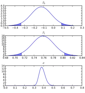
Figure 2: Marginal posterior density plots for the regression coefficients in example 1.

The parameter associated with variable 12, ˆβ1, is estimated as a positive value, 0.7587, with a 95% credible interval [0.7139, 0.8035]. We note that zero is not contained in the credible interval, hence the crop yield increases with higher values of variable 12. The marginal posterior densities (Figure2) can be created using

breg.plot()

This clearly shows this effect is far from zero. 3.2. Example 2: Log-linear model

The data analysed in this example are the number of nutgrass shoots counted, in randomly scattered quadrats, at weekly intervals, during the growing season. A log linear model is used; log(count) =β0+β1week (13)

where the intercept, β0, is expected to be positive in value, as nutgrass is always present in this study site, andβ1 is also expected to be positive as the population of nutgrass increases during the growing season.

For the log-linear model, seeGelman, Carlin, Stern, and Rubin(2004), theithobservationyi, fori= 1,2, . . . , n, is generated as follows

p(yi|µi) =

µyi

i exp(−µi)

µi!

(23)

with

log(µi) =xTi β, wherexT_i is theithrow of the (n×k) matrixX.

The joint posterior distribution for the unknown parameterβ is given by

p(β|y,X)∝p(y|β,X)×p(β), (15) where p(y|β,X) is the joint pdf for y conditional on the β and X, and p(β) denotes the priorpdf forβ.From Equation 14it is apparent that

p(y|β,X) = n Y i=1 µyi i exp(−µi) µi! . Apriori we assume that

β∼N(β,V−1).

To sample from Equation15, a random walk MH algorithm is implemented, where the can-didateβ∗, at each iteration, is sampled following

β∗ ∼Nβj−1,Ω, (16) where

β0=βnls= arg min (y−exp (Xβ))2 and Ω−1 =− n X i=1 expxT_i βnls xixTi .

The example code forPyMCMCuses twoPythonlibraries,NumpyandScipy, which the user must have installed to run the code.

As before, the code begins by importing the required packages:

import os

from numpy import random, loadtxt, hstack, ones, dot, exp, zeros, outer, diag from numpy import linalg

from pymcmc.mcmc import MCMC, RWMH, OBMC from pymcmc.regtools import LinearModel from scipy.optimize.minpack import leastsq

The import statements are followed by the definition of a number or required functions. A functionminfunc used in the non-linear least squares routine:

def minfunc(beta, yvec, xmat ):

return yvec - exp(dot(xmat, beta))

A function prior to evaluate the log of the prior pdf β. and a function logl defining the log-likelihood function:

(24)

def prior(store):

mu = zeros(store['beta'].shape[0])

Prec = diag(0.005 * ones(store['beta'].shape[0]))

return -0.5 * dot(store['beta'].transpose(), dot(Prec, store['beta'])) def logl(store):

xbeta = dot(store['xmat'], store['beta']) lamb = exp(xbeta)

return sum(store['yvec'] * xbeta - Lamb)

As in the variable selection example, store is a Python dictionary used to store all the information of interest that needs to be accessed by functions that are called from the MCMC sampler. For example, the function logl uses store[‘beta’] which provides access to the vector β.

A function posterior which evaluates the log of the posterior pdf forβ:

def posterior(store):

return logl(store) + prior(store)

A function llhessian which returns the hessian for the log-linear model:

def llhessian(store, beta): nobs = store['yvec'].shape[0] kreg = store['xmat'].shape[1]

lamb = exp(dot(store['xmat'], beta)) sum = zeros((kreg, kreg))

for i in xrange(nobs):

sum = sum + lamb[i] * outer(store['xmat'][i], store['xmat'][i]) return -sum

Following the function definitions, the main program begins with the command to set the random seed:

random.seed(12345)

and the set up of the data:

data = loadtxt('count.txt', skiprows = 1) yvec = data[:, 0]

xmat = data[:, 1:data.shape[1]]

xmat = hstack([ones((data.shape[0], 1)), xmat]) data ={'yvec':yvec, 'xmat':xmat}

Bayesian regression is used to initialise the non-linear least squares algorithm:

bayesreg = LinearModel(yvec, xmat) sig, beta0 = bayesreg.posterior_mean()

(25)

The functionleastsq fromScipy is used to perform the non-linear least squares operation:

init_beta, info = leastsq(minfunc, beta0, args = (yvec, xmat)) data['betaprec'] =-llhessian(data, init_beta)

scale = linalg.inv(data['betaprec'])

Initialise the random walk MH algorithm:

samplebeta = RWMH(posterior, scale, init_beta, 'beta')

Finally, setup and run the sampling scheme. Note that the sampling algorithm is run for 20000 iterations and the first 4000 is discarded. The MCMC scheme has only one block and is a MH sampling scheme:

ms = MCMC(20000, 4000, data, [samplebeta], loglike = (logl, xmat.shape[1], 'yvec')) ms.sampler()

A summary of the model fit can be produced using the output function:

ms.output()

---The time (seconds) for the Gibbs sampler = 7.47 Number of blocks in Gibbs sampler = 1

mean sd 2.5% 97.5% IFactor beta[0] 1.14 0.0456 1.05 1.23 13.5 beta[1] 0.157 0.00428 0.148 0.165 12.2 Acceptance rate beta = 0.5625

BIC = -7718.074

Log likelihood = 3864.453

It can be seen from the output that estimation is very fast (7.5 seconds), and that both β0 and β1 are positive values, with ˆβ0 = 1.14 [1.05, 1.23] and ˆβ1 = 0.157 [0.148, 0.165].

Summary plots can also be produced (Figure 3):

ms.plot('beta')

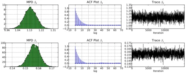
The marginal posterior densities of these estimates (Figure3) confirm that both estimates are far from zero. The ACF plots (Figure3) and low inefficiency factors (seeChib and Greenberg (1996) for details on inefficiency factors) of 13.5 ( ˆβ0) and 12.2 ( ˆβ1) show that autocorrelation in the sample is relatively low for an MCMC sampler.

(26)

0.96 1.04 1.13 1.22 1.31 02 4 6 8 10 MPD β0 10 0 10 20 30 40 50 60 70 lag 0.2 0.00.2 0.4 0.6 0.81.0 ACF Plot β0 0 5000 10000 Iteration 0.95 1.001.05 1.101.15 1.201.25 1.301.35 Trace β0 0.14 0.15 0.160.16 0.17 0 20 40 60 80 100 MPD β1 10 0 10 20 30 40 50 60 70 lag 0.2 0.00.2 0.4 0.6 0.81.0 ACF Plot β1 0 5000 10000 Iteration 0.135 0.140 0.145 0.150 0.155 0.160 0.165 0.170 0.175 Trace β1

Figure 3: Plots of the marginal posterior density, autocorrelation and trace plots for the MCMC estimation of the log linear model in Example 2. Note summaries are calculated after removing the burn in.

3.3. Example 3: First order autoregressive regression

The final example demonstrates first order autoregressive regression using a simulated data set, with 1000 observations and 3 regressors.

The linear regression model, with first order autocorrelated serial correlation in the residuals, seeZellner(1971) is defined such that thetth observation,yt,fort= 1,2, . . . , n,

yt=xTtβ+εt, (17)

with

εt=ρεt−1+νt; νt∼i.i.d.N(0, σ2), (18) wherextis a (k×1) vector of regressors,βis a (k×1) vector of regression coefficients,ρis a damping parameter andνtis an independent identically normally distributed random variable with a mean of 0 and a variance of σ2. Under the assumption that the process driving the errors is stationary, that is |ρ| < 1, and assuming that the process has been running since time immemorial then Equation17and Equation 18 can be expressed as

y=Xβ+ε; ε∼N0, κ−1Ω−1, (19) where Ω=              1 −ρ 0 0 · · · 0 −ρ 1 +ρ2 −ρ 0 . .. 0 0 −ρ 1 +ρ2 . .. . .. ... 0 0 . .. . .. −ρ 0 .. . ... . .. −ρ 1 +ρ2 −ρ 0 0 · · · 0 −ρ 1              .

(27)

Further, if we factoriseΩ=LLT,using the Cholesky decomposition, it is straightforward to deriveL,where L=              1 −ρ 0 0 · · · 0 0 1 −ρ . .. ... 0 0 0 . .. ... ... ... .. . . .. ... ... ... 0 .. . . .. ... ... 1 −ρ 0 0 · · · 0 p1−ρ2              .

Pre-multiplying Equation19, by Lgives ˜

y=Xβ˜ +ε˜, (20) wherey˜=LTy,X˜ =LTX and ˜ε=LTε.Note that ε∼N(0, κ−1I).

The joint posterior distribution for the full set of unknown parameters is

p(β, κ, ρ|y)∝p(y|β, κ, ρ)×p(β, κ)×p(ρ), (21) where p(y|β, κ, ρ) is the joint pdf of y conditional on β, κ, and ρ, p(β, κ) is the joint prior pdf for β and κ, and p(ρ) denotes the prior density function for ρ. The likelihood function, which is defined following Equation 17and Equation 18 is defined as follows

p(y|β, κ, ρ) ∝ κn/2|Ω|1/2_exp₋κ 2(y−Xβ) T _Ω_(y₋_Xβ) = κn/2|Ω|1/2_exp₋κ 2 ˜ y−Xβ˜ Ty˜−Xβ˜ . = κn/21−ρ21/2exp −κ 2 ˜ y−Xβ˜ T y˜−Xβ˜ . (22)

For the analysis a normal-gamma prior is assumed forβ andκ, such that β|κ∼Nβ, κ−1, κ∼G _ν 2, S 2 . (23)

It follows from Equation22and Equation23that samplingβandκconditional onρis simply equivalent to sampling from a linear regression model with a normal-gamma prior. A beta prior is assumed for ρ there by restricting the autocorrelation of the time series to be both positive and stationary. Specifically

ρ∼ Be(α, β).

A MCMC sampling scheme, for the posterior distribution in Equation 21, defined at iteration

j is as follows:

1. Sampleβ(j), κ(j) from p(β, κ|y, ρ(j−1)).

2. Sampleρ(j) from p(ρ|y,β, κ).

The code for this model follows the structure of the previous examples, and begins by im-porting the required packages:

(28)

from numpy import random, ones, zeros, dot, hstack, eye, log from scipy import sparse

from pysparse import spmatrix

from pymcmc.mcmc import MCMC, SliceSampler, RWMH, OBMC, MH, CFsampler from pymcmc.regtools import LinearModel

As this example uses simulated data the first function is used to derive this data:

def simdata(nobs, kreg):

xmat = hstack((ones((nobs, 1)), random.randn(nobs, kreg - 1))) beta = random.randn(kreg)

sig = 0.2 rho = 0.90

yvec = zeros(nobs) eps = zeros(nobs)

eps[0] = sig ** 2 / (1. - rho ** 2) for i in xrange(nobs - 1):

eps[i + 1] = rho * eps[i] + sig * random.randn(1) yvec = dot(xmat, beta) + eps

return yvec, xmat

Next, define a function that calculates ˜y andX˜:

def calcweighted(store):

nobs = store['yvec'].shape[0]

store['Upper'].put(-store['rho'], range(0, nobs - 1), range(1, nobs)) store['Upper'].matvec(store['yvec'], store['yvectil'])

for i in xrange(store['xmat'].shape[1]):

store['Upper'].matvec(store['xmat'][:, i], store['xmattil'][:, i])

Note that LT is updated based on the latest iteration in the MCMC scheme. Further,LT is stored in the Python dictionary storeand is accessed using the key‘Upper’. It is stored in sparse matrix format using the library Pysparse.

Next define a function that is used to sample β,from its conditional posterior distribution:

def WLS(store):

calcweighted(store)

store['regsampler'].update_yvec(store['yvectil']) store['regsampler'].update_xmat(store['xmattil']) return store['regsampler'].sample()

Now define functions to evaluate the log-likelihood (loglike), the log of the prior pdf for ρ

(29)

def loglike(store):

nobs = store['yvec'].shape[0] calcweighted(store)

store['regsampler'].update_yvec(store['yvectil']) store['regsampler'].update_xmat(store['xmattil'])

return store['regsampler'].loglike(store['sigma'], store['beta']) def prior_rho(store):

if store['rho'] > 0. and store['rho'] < 1.0: alpha = 1.0

beta = 1.0

return (alpha - 1.) * log(store['rho']) + (beta - 1.) * \ log(1.-store['rho'])

else:

return -1E256

def post_rho(store):

return loglike(store) + prior_rho(store)

The main program begins by setting the seed and constructing the Python dictionary data, which is used to store information that will be passed to functions that are called from the MCMC sampler:

random.seed(12345) nobs = 1000

kreg = 3

yvec, xmat = simdata(nobs, kreg)

priorreg = ('g_prior', zeros(kreg), 1000.0)

regs = LinearModel(yvec, xmat, prior = priorreg) data ={'yvec':yvec, 'xmat':xmat, 'regsampler':regs} U = spmatrix.ll_mat(nobs, nobs, 2 * nobs - 1) U.put(1.0, range(0, nobs), range(0, nobs)) data['yvectil'] = zeros(nobs)

data['xmattil'] = zeros((nobs, kreg)) data['Upper'] = U

Initial values for σ and β are set using Bayesian regression:

bayesreg = LinearModel(yvec, xmat) sig, beta = bayesreg.posterior_mean()

The parameters σ and β are jointly sampled using the closed form class:

simsigbeta = CFsampler(WLS, [sig, beta], ['sigma', 'beta'])

(30)

rho = 0.9

simrho = SliceSampler([post_rho], 0.1, 5, rho, 'rho')

In this example, there are two blocks in the MCMC sampler. The code:

blocks = [simrho, simsigbeta]

constructs a Python list that contains the class instances that define the MCMC sampler. In particular, it implies that the MCMC sampler consists of two blocks. Further, ρ will be the first element sampled in the MCMC scheme.

Finally, the sampler can be initialised and sampling undertaken:

loglikeinfo = (loglike, kreg + 2, 'yvec')

ms = MCMC(10000, 2000, data, blocks, loglike = loglikeinfo) ms.sampler()

The MCMC sampler is run for 10000 iterations and the first 2000 are discarded. A summary can be generated by the output command:

ms.output()

The time (seconds) for the Gibbs sampler = 27.72 Number of blocks in Gibbs sampler = 2

mean sd 2.5% 97.5% IFactor beta[0] -0.523 0.0716 -0.653 -0.373 3.5 beta[1] 1.85 0.00508 1.84 1.86 3.56 beta[2] 0.455 0.00505 0.445 0.465 3.75 sigma 0.217 0.00489 0.207 0.226 3.5 rho 0.901 0.0155 0.872 0.932 3.67

Acceptance rate beta = 1.0 Acceptance rate sigma = 1.0 Acceptance rate rho = 1.0 BIC = -331.398

Log likelihood = 182.969

The total time of estimation is approximately 28 seconds. From the inefficiency factors it is clear that the algorithm is very efficient.

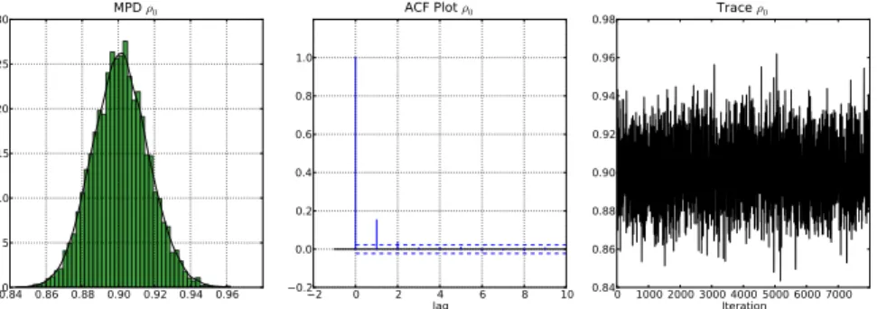
Summary plots generated usingms.plot(‘rho’) (Figure 4) provide the marginal posterior density, autocorrelation plot and the trace plot for the iterates.

(31)

0.84 0.86 0.88 0.90 0.92 0.94 0.960 5 10 15 20 25 30 MPD ρ0 2 0 2 _lag4 6 8 10 0.2 0.0 0.2 0.4 0.6 0.8 1.0 ACF Plot ρ0 0 1000 2000 3000 4000 5000 6000 7000_Iteration 0.84 0.86 0.88 0.90 0.92 0.94 0.96 0.98 Trace ρ0

Figure 4: Marginal posterior density, autocorrelation function and trace plot based on the MCMC analysis for Example 3. Note summaries are calculated after removing the burnin.

4. Using

PyMCMC

efficiently

The fact that MCMC algorithms rely on a large number of iterations to achieve reasonable results and are often implemented on very large problems, limits the practitioner’s choice of a suitable environment, in which they can implement efficient code. This efficiency comes through an understanding of what makes a simulation efficient MCMC sampler, and also the ability to produce computationally efficient code. Interestingly, the two are related. To achieve both simulation and computationally efficient code in MCMC samplers it is often extremely important that large numbers of parameters are sampled in blocks, rather than the alternative of a single move sampler. From the perspective of simulation efficiency it is well known that individually sampling correlated parameters induces correlation in the resultant Markov chain and thus leads to a poorly mixing sampler. A classic example in the literature uses simulation smoothers to jointly sample the state vector in a state space model; see for example Carter and Kohn (1994) and de Jong and Shephard (1995). Whilst implementing a simulation smoother is required to achieve simulation efficient code, the sequential nature of their implementation often renders higher level languages impractical for large problems and thus forces the analyst to write their entire code in a lower level language. This is an inefficient use of time as usually only a small percentage of code needs to be optimised. This drawback is easily circumvented in PyMCMC as Python makes it easy to use a lower level language to write the specialised module and use the functions directly from Python. This ensures PyMCMC’s modules can be used for rapid development from Pythonand lower level languages are only resorted to when necessary.

This section aims to provide guidelines for producing efficient code withPyMCMC. We discuss alternative external libraries that are available to the user for producing efficient code using

PyMCMC. Despite the ease of writing specialised modules this should not be the first resort of the user. Instead, one should ensure that the Python code is as efficient as possible using the resources available with Python.

Arguably, the first thing the user of PyMCMCshould concentrate on when optimising their

PyMCMC code is to ensure they use as many inbuilt functions and libraries as possible. As most high performance libraries are written inC orFortranthis ensures that computationally expensive procedures are computed using code from compiled languages. Python users, and hencePyMCMCusers, have an enormous resource of Scientific libraries available to them as

(32)

a result of the popularity of Pythonin the scientific community. Two of the most important libraries for most users will quite possibly beNumpyandScipy. Making use of such libraries is one of the best ways of avoiding large loops in procedures that are called from the MCMC sampler. If a large loop is used inside a function that is called from inside the MCMC sampler then this could mean that a large proportion of the total computation is being done by Python, rather than a library that was generated from optimised compiled code. This can have a dramatic effect on the total computation time. As a simple and somewhat trivial example we modify Example 2 from Section 3.2 so that a loop is explicitly used to calculate the log likelihood.

def logl(store): suml=0.0

for i in xrange(store['yvec'].shape[0]):

xbeta=dot(store['xmat'][i,:],store['beta']) suml=suml+store['yvec'][i] * xbeta - Exp(xbeta) return suml

Whilst the two functions to calculate the log-likelihood are mathematically equivalent, the one with the explicit loop is substantially slower. Specifically, the time taken for the MCMC sampler went from 7.3 seconds to 130.19 seconds. As such, this minor modification leads to an approximate 18-fold decrease in the speed of the program.

If the use of an an inbuilt function is not possible and the time taken from the program is unacceptable then there are several alternative solutions available to the user. One such solution is to use the package Weave, which is a part of the Scipy library, to write inline C code which will accelerate the problem area in the code. An example is given below.

def logl(store): code = """

double sum = 0.0, xbeta; for(int i=0; i<nobs; i++){

xbeta = 0.0;

for(int j=0; j<kreg; j++){ xbeta += xmat(i,j) * beta(j); }

sum += yvec(i) * xbeta - exp(xbeta); }

return_val = sum; """

yvec = store['yvec'] xmat = store['xmat']

nobs, kreg = xmat.shape beta = store['beta']

return weave.inline(code,['yvec','xmat', 'beta','nobs','kreg'],\

compiler='gcc',type_converters=converters.blitz)

The total time taken forWeaveversion is 4.33 seconds. The reason for the speed increase over the original version that uses Numpyfunctions is the Weave version avoids the construction of temporary matrices that are typically a by product of overloaded operators.

(33)

Another alternative, which is our preferred approach, is to use thePythonmodule F2py; see Peterson(2009) for further details. F2py allows for the seamless integration of Fortran and Python code. Following on using the same trivial example we use the following Fortran77 code. This example requires that the user have basic linear algebra subprograms (BLAS) and preferably also the automatically tuned linear algebra software (ATLAS).

c fortran 77 code used to calculate the likelihood of a log c linear model. Subroutine uses BLAS.

subroutine logl(xb,xm,bv,yv,llike,n,k) implicit none

integer n, k, i, j

real*8 xb(n),xm(n,k), bv(k), yv(n), llike real*8 alpha, beta

cf2py intent(in,out) logl cf2py intent(in) yv

cf2py intent(in) bv cf2py intent(in) xmat cf2py intent(in) xb

alpha=1.0 beta=0.0

call dgemv('n',n,k,alpha,xm,n,bv,1,beta,xb,1) llike=0.0

do i=1,n

llike=llike+yv(i)*xb(i)-exp(xb(i)) enddo

end

In UNIX type environments, such as Linux and OSX the code is compiled with the following command (Windows users see Section4.1):

f2py -c loglinear.f -m loglinear -lblas -latlas

The loglinear library can then be imported as a python module, and the functionloglaccessed as a standard python function:

import loglinear

print loglinear.logl.__doc__

logl - Function signature:

llike = logl(xb,xm,bv,yv,llike,[n,k]) Required arguments:

(34)

xb : input rank-1 array('d') with bounds (n) xm : input rank-2 array('d') with bounds (n,k) bv : input rank-1 array('d') with bounds (k) yv : input rank-1 array('d') with bounds (n) llike : input float

Optional arguments: n := len(xb) input int k := shape(xm,1) input int Return objects:

llike : float

Note that this function requires as input xb a rank-1 array of length n. We add this to the

data dictionary:

data['xb']=zeros(yvec.shape[0])

The array data[‘xb’] is a work array used for the calculation ofXβ.As it is stored in the Python dictionary data it is only created once rather that each time the function logl is called.

It is useful to pass arrays stored in column major order toF2pyfunctions since this is what is used in Fortran, rather than thePython default, which is row major order the default for the C programming language. This can be achieved using the Numpyfunctionasfortranarray:

data['xmatf']=asfortranarray(xmat)

Ifstore[‘xmat’] were passed to the functionloglinear.loglthenF2pywill automatically produce a copy and convert it to column major order each time the functionlogl is called. The function logl can now be rewritten as:

import loglinear def logl(store):

loglike=array(0.0)

return loglinear.logl(store['xb'],store['xmatf'], store['beta'],store['yvec'],loglike)

The total time for the MCMC sampler when usingF2pyis 4.03 seconds. This is slightly faster that the version that uses Weave, where most likely the small gain can be attributed to the use of ATLAS.

The user has many other choices available to them for writing specialised extension modules. For example, if it is the preference of the user it is not much more difficult to use F2py to compile procedures written in C, which then can be used directly from Python. Another popular library that can be used to marry C, as well asC++, code with Pythonis SWIG. In our opinion SWIG is more difficult than f2py for complicated examples. The user may also opt to manually call C andC++routines usingPythonand Numpy’sCapplication interface. Another option for C++ users is to use Boost Python. These alternative approaches are beyond the scope of this paper.

(35)

4.1. Compiling code in Windows

The previous section described how one might go about using PyMCMCefficiently. To do this, access to a compiler is necessary. Under most flavours of UNIX, this should pose no problem, but under Microsoft Windows this can be more difficult. This section provides some brief guidelines to an approach we found workable under Windows.

In order to runPyMCMC,Python,NumpyandScipyare all required, but to have a reasonable developer experience under Windows, we suggest a few additional packages, all of which are freely available:

• mingw (http://www.mingw.org/) which provides, among other things, the GNU com-piler suite. The user should choose at least gccand g++.

• msys (http://www.mingw.org/wiki/MSYS) which provides a set of GNU utilities com-monly found on Linux. This will make building and compiling code more manageable under Windows.

• ipython(http://ipython.scipy.org/moin/), an interactive interface toPython, which can be used as an alternative to the idle interface that is distributed with Python.

• pyreadline(http://ipython.scipy.org/moin/PyReadline/Intro), which provides Windows readline capabilities for IPython.

• gfortran(http://gcc.gnu.org/wiki/GFortranBinaries), which provides a native Windows Fortran compiler.

Once these additional utilities are installed, it should be possible to compile code in different languages. To test that Weaveworks as expected, make sure that the mingwbin directory is in your path, and try the following code:

import scipy.weave a=100

scipy.weave.inline('printf("a=%d\\n",a);',['a'],verbose=1)

The output should be similar to:

In [4]: scipy.weave.inline('printf("a=%d\\n",a);',['a'],verbose=1) <weave: compiling>

No module named msvccompiler in numpy.distutils; trying from distutils Compiling code...

Found executable c:\mingw\bin\g++.exe finished compiling (sec): 2.73600006104 a=100

F2py requires a Fortran compiler. To set this up under Windows, follow the instructions at http://www.scipy.org/F2PY Windows, and make sure the simple example provided works on your system. The examples presented above additionally requireBLASorATLASto be avail-able. This can be built under windows (see instructions at http://www.scipy.org/Installing SciPy/Windows, for example). To check that F2py and

(36)

subroutine dgemveg() REAL*8 X(2, 3) /1.D0, 2.D0, 3.D0, 4.D0, 5.D0, 6.D0/ REAL*8 Y(3) /2.D0, 2.D0, 2.D0/ REAL*8 Z(2) CALL DGEMV('N', 2, 3, 1.D0, X, 2, Y, 1, 0.D0, Z, 1) PRINT *, Z

end subroutine dgemveg

Set the location of your ATLAS libraries appropriately, and ensure that gfortran is in your path and compile. The following provides a template:

ATLAS_LIB_DIR="/d/tmp/pymcmc_win_install/BUILDS/lib" export PATH=${PATH}:\

/c/Program\ Files/gfortran/libexec/gcc/i586-pc-mingw32/4.6.0:\ /c/Program\ Files/gfortran/bin:/c/python26

python /c/Python26/Scripts/f2py.py -c -m foo \ --fcompiler=gfortran \

blas_eg.f90 -L${ATLAS_LIB_DIR} -lf77blas -latlas -lg2c

This should produce aPythondll (foo.pyd), which can be imported into Python:

import foo dir(foo)

print foo.__doc__ foo.dgemveg()

5. PyMCMC

interacting with

R

There are many functions from theRstatistical language (R Development Core Team 2010) that can be useful in Bayesian analysis. The RPy2 (Gautier 2011) Python library can be used to integrateRfunctions into PyMCMCprograms. These can be accessed inPyMCMC

through theRPy2 Python library. As an example, consider the log linear model described in Section3.2. The random walk MH requires the specification of a candidate density function Equation 2 and an initial value. The Rfunctions glm and summary.glm can be used to set this to the maximum likelihood estimate ˆβ and the unscaled estimated covariance matrix of the estimated coefficients. The relevant code is summarised below:

import rpy2.robjects as robjects

def initial_values(yvec,xmat): ry = robjects.FloatVector(yvec)

rv = robjects.FloatVector(xmat[:,1:].flatten()) rx = robjects.r['matrix'](rv, nrow=xmat.shape[0],

(37)

robjects.globalenv['y'] = ry robjects.globalenv['x'] = rx

mod = robjects.r.glm("y~x", family="poisson") init_beta = array(robjects.r.coefficients(mod)) modsummary = robjects.r.summary(mod)

scale = array(modsummary.rx2('cov.unscaled')) return init_beta,scale

random.seed(12345)

data=loadtxt('count.txt',skiprows=1) yvec=data[:,0]

xmat=data[:,1:data.shape[1]]

xmat=hstack([ones((data.shape[0],1)),xmat])

data={'yvec':yvec,'xmat':xmat}

init_beta,scale=initial_values(yvec,xmat)

samplebeta=RWMH(posterior,scale,init_beta,'beta')

ms=MCMC(20000,4000,data, [samplebeta],loglike=(logl,xmat.shape[1],'yvec')) ms.sampler()

ms.CODAoutput(filename="loglinear_eg", parameter="beta")

It may also be useful to take advantage of the many MCMC analysis functions in R and associated packages. To facilitate this, PyMCMC includes a CODA (Plummer et al. 2006) output format which can easily be read intoRfor further analysis. A sample Rsession after

PyMCMCmight look like:

library(coda) aa <- read.coda("loglinear_eg.txt","loglinear_eg.ind") plot(aa) summary(aa) raftery.diag(aa) xyplot(aa) densityplot(aa) acfplot(aa,lag.max=500)

6. Obtaining

PyMCMC

The source code forPyMCMCis held in agit repostitory, and can be cloned by