Quantification and interpretation of glacier elevation changes

(1)

Quantiﬁcation and interpretation

of glacier elevation changes

Christopher Nuth

Department of Geosciences

University of Oslo

A thesis submitted for the degree of Philosophiae Doctor (PhD)

(2)

© Christopher Nuth, 2011

Series of dissertations submitted to the

Faculty of Mathematics and Natural Sciences, University of Oslo No. 1062

ISSN 1501-7710

reproduced or transmitted, in any form or by any means, without permission.

Cover: Inger Sandved Anfinsen. Printed in Norway: AIT Oslo AS. Produced in co-operation with Unipub.

The thesis is produced by Unipub merely in connection with the

thesis defence. Kindly direct all inquiries regarding the thesis to the copyright holder or the unit which grants the doctorate.

(3)

Abstract

Glaciers, ice caps and ice sheets constitute a large reservoir in the global hydrolog-ical cycle and provide a coupling between climate and sea-level. Observations of glacial change is important for constraining their contribution to sea-level fluctua-tions and to better understand the interacfluctua-tions between glaciers and climate. This thesis focuses on glacier observations through measurements of elevation change. The research in this thesis is oriented towards the methodological detection of elevation changes using remote sensing techniques. The quality of glacier elevation change measurements is dependent on controlling the potential errors and biases within the data. Therefore, one aspect is focused on a universal co-registration method for elevation products and further identification and correction of biases that remain, specifically in satellite stereo products.

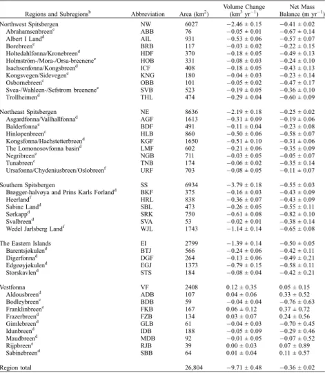
For glaciological studies, elevation changes require conversion into volume and mass changes. This is sometimes complicated when the data available is not spa-tially continuous and/or temporally consistent. Therefore, another aspect of this thesis explores methods for estimating regional glacier volume change. Speciﬁcally, Svalbard glacial contribution to sea-level has been estimated using regionalization techniques from scattered elevation measurements over roughly two time epochs. We observed that Svalbard glaciers over the past few decades have had a negative mass balance, contributing approximately 0.026 mm per year to the oceans. Dur-ing the past few years, the sea-level contribution from Svalbard glaciers decreased slightly to 0.013 mm per year.

Interpretations of elevation changes are convoluted by their dependence on cli-matic and dynamic forces operating on glacier systems. The last aspect of this thesis experiments with surface mass balance modelling for quantifying the cli-matic component of an elevation change. Combining this with observed elevation changes using theory of mass continuity can yield estimates of the calving flux of icebergs into the ocean. We observed on one particular fast flowing glacier in Svalbard that the average calving flux in the 1966-1990 epoch increased in the 1990-2007 epoch.

(4)

(5)

Acknowledgements

A thesis comprises more than just the words on the following 141 pages. A thesis con-tains ideas shared and developed with colleagues. A thesis comprises many hours of field work providing shared adventures and experiences that create strong friendships. A thesis involves many hours of stress and struggle that work its way into our personal lives. This thesis would not be possible without the support and guidance from my super-visors. Jack Kohler introduced me to glaciology and took me under his wing after a rather short meeting 5 years ago in Oslo Central Station (over a cup of coffee, of course!). He has been my mentor ever since and I owe much of my knowledge to him, and not to forget all the fun and frustrations of the yearly field work. Jon Ove Hagen has also men-tored me from Day 1. With his years of experience in glaciology and nonchalant approach towards fieldwork, he has shaped many of the ideas contained in this thesis and led me on countless adventures. Thomas Vikhamar Schuler believed in one original idea of this thesis, and guided me throughout the process. Without his perseverance and patience, I

would have never learned as much as I have. Andreas K¨a¨ab is the remote sensing mentor

that opened my eyes to proper techniques and methods as well as guiding me towards better and more interesting science.

I must also acknowledge the numerous colleagues and friends at the Dept. of Geosciences (UiO) and the Norwegian Polar Institute who have provided great working conditions both in the oﬃce and the ﬁeld. In particular, Geir Moholdt has taught me much through our time together sharing ideas and writing papers. Ola Brandt has been a great

men-tor in the field and the office. Bas Altena, Anne Chapuis and Mats Björkman have

been great friends in the field and office. I am grateful to Kimberly Casey who took on the tedious job of proofing parts of this thesis. And not to forget the numerous oth-ers (Karsten, Thorben, Torborg, Tobi and Anna) for all the interesting discussions both scientific and non scientific that made lunch breaks interesting and coffee breaks plentiful. I have to also thank my family for everything they have provided for me. Mom for pushing me into education when I least wanted to. Dad for supporting me whenever I needed an extra hand. Tara for holding high spirits and interest in this work which some-times can feel meaningless. Last, I thank my beloved Ann-Live for her loving support and the final part of this thesis is, of course, dedicated to Trym.

(6)

1 Introduction

Glaciers, ice-caps and ice sheets together cover≈14.5 million km2_{of the Earth’s surface} and have a potential to raise sea level1_{up to}_≈_{64 m (Lemke et al., 2007). The relation} between land-ice and other components of the present climate system is complex and large regional variability persists in the mass change of glaciers. It still remains unclear whether gain of mass in the accumulation areas is compensating for some of the loss at the peripherals (Walsh and others, 2005). The extensive volume of land-ice adjusts in response to climate, radiative forcing and ice dynamics and further represents a coupling between climatic change and sea-level fluctuation. As temperature and melt increase, the global area of ice declines reducing the albedo, the reflectivity of the Earth’s surface. This allows more solar energy to be absorbed at the Earth’s surface, further increasing temperature and melt (Barry, 2002). In addition, as the magnitude and area of surface melt increases on a glacier, the increased melt water potentially reaching the base of the glacier increases the sliding velocity (Iken and Bindschadler, 1986; Bartholomaus et al., 2008; Schoof, 2010) and thus the calving flux of ice into the ocean (Zwally et al., 2002a). Therefore, monitoring changes of glaciers, ice-caps and ice sheets is important in determining the past and present day contribution to sea level fluctuation and to better characterize the present day changes in relation to climatic fluctuations.

The principle parameter that characterizes glacier change is the mass balance, or the change in water equivalent volume of the glacier within some deﬁned time interval.

1_{assuming an ocean area of 362 million km}2_{, an ice density of 917 kg m}−3_{, a seawater density of}

(10)

1. INTRODUCTION

Generally, this mass balance may be divided into three components: the surface and basal mass balance and the mass loss due to calving icebergs. Proxies for the seasonal or annual mass balance include the equilibrium line altitude (ELA) which represents the elevation that divides the ablation and accumulation zones on the glacier or the accumulation area ratio (AAR), the percentage of area above the ELA. Proxies for the longer temporal state of glaciers can be reﬂected in ﬂuctuations of the glacier front position, inherently a function of mass balance and proxy for temperature (e.g. Oerlemans, 2005).

Monitoring glacier changes directly from the ground include measurements of the surface mass balance, velocity and/or elevation and terminus changes. The surface mass balance is determined by stakes drilled into the ice surface. The height from the glacier surface to the top of the stake is measured on a seasonal and/or annual interval and the change in this height multiplied by the density of the snow/ice results in the mass change at the stake (Østrem and Brugman, 1991). The point measurements are then integrated (extrapolated) over the entire glacier surface, commonly using the area-altitude distribution (also called the hypsometry). Alternately, extrapolation of point measurements can be accomplished by empirically or analytically modelling compo-nents of the mass balance (Hock, 2003; Arnold et al., 2006; Schuler et al., 2007; Sicart et al., 2008; Schuler et al., 2008). Glacier velocity may also be measured by deter-mination of the stake positions through time, commonly using the global navigation satellite system (GNSS) with code (less accurate) and differential (more accurate) based receivers. Estimating the glacier flux in terms of calving icebergs require ice thickness measurements (acquired using radar and seismic techniques or directly drilling through the ice) and an assumption (or measurement) of the velocity profile with depth. Last, GNSS techniques on the ground may be used to measure the terminus position and glacier surface elevation that can help determine the volume change of a glacier.

The techniques of measuring the Earth’s surface through remote sensing has pro-vided the ability to measure numerous glacier parameters that are related to both the instantaneous and temporally averaged mass balance of the glacier. Over longer time periods (greater than a few years), the volume change of a glacier can be measured by comparing measurements of surface elevation obtained by either photogrammetric principles applied to stereo-optical imagery (either aerial or satellite-borne) (e.g. K¨a¨ab,

(11)

2005), interferometric techniques of radar imagery (e.g. Farr et al., 2007) or altimet-ric acquisition methods (e.g. Echelmeyer et al., 1996). Indirect proxies of the longer time glacier mass balance can be derived by remote sensing through measurements of area and length changes from terrestrial, aerial and satellite imagery comparison (e.g. Hoelzle et al., 2007; Andreassen et al., 2008). On a shorter time scale, snow line altitude, a proxy for the ELA, and the AAR can be detected using either visible or radar images which are related to the seasonal or annual surface mass balance of a glacier (e.g. König et al., 2004; Mathieu et al., 2009; Barcaza et al., 2009). Recently, international collaborations efforts have been concentrated on deriving a global glacier database (The GLIMS project, www.GLIMS.org) based upon measurements from space that help record the increasing amount of proxy data such as area changes and snow-line locations (Raup et al., 2007). Glacier velocity can also be measured remotely using either interferometric (Kwok and Fahnestock, 1996) or image matching (Joughin, 2002; Kääb et al., 2005) techniques, both dependent on the magnitude of the movement be-tween two acquisitions. Translation of velocities into fluxes require knowledge of the ice thickness (cross sectional area) which is reliant on ground-based remote sensing tech-nologies. Similarly, an assumption or measurement of the velocity profile with depth is required to translate surface velocities into calving fluxes.

The goals of many of these measurements and applied techniques are to better define the contribution of glaciers, ice-caps and ice sheets to sea-level change and to better define the processes that relate glacier behavior to driving and determining forces such as meteorology and climate, geology and hydrology. This thesis combines both direct and remotely sensed measurements in order to quantify glacier changes, analyze methods and approaches from which to determine those glacier changes, and if possible, offer quantifiable interpretations of the changes. With increasing capability to monitor glaciers continuously from space, observed glacier changes will help constrain models to predict the future behavior of glaciers.

(12)

2 Motivation and Objectives

The first glacier inventory of Svalbard classified 2229 glaciers making up≈36,000 km2_, about 60% of the land area (Hagen et al., 1993). The archipelago contains small valley glaciers, larger tidewater glaciers, smaller ice fields and ice caps, many of which are polythermal in nature, exhibit surge-like behavior and some relic fast flowing glacier units. Svalbard contains two of the longest continuous direct mass balance time series (1967-present) in the Arctic, Midtre Lóvenbreen and Austre brøggerbreen located in western Svalbard. About 13 other small glaciers, mainly located in the central or south part of the archipelago have direct mass balance measurements available (Hagen et al., 2003b). Since 2004 and 2007, continuous mass balance measurements have been carried out on the largest ice mass in Svalbard, Austfonna (Moholdt et al., 2010a), and its smaller sibling Vestfonna (Möller et al., subm.), respectively. Previous estimates of the archipelagos mass balance have mainly been restricted to extrapolations of these direct surface mass balance estimates.

The location of Svalbard at the transition boundary between the tail end of the warm Atlantic current that transports heat from the tropics to the poles and the colder arctic atmosphere creates regionally variable meteorological conditions. This makes extrapolations of direct mass balance measurements significantly difficult due to under-sampling both in space and with elevation (Hagen et al., 2003b). Therefore, previous estimation of Svalbard’s present-day sea-level equivalent (SLE) contribution has varied between 0.01 SLE yr−1_{(Hagen et al., 2003b), 0.038 SLE yr}−1_{(Hagen et al., 2003a) and} 0.056 SLE yr−1 _{(Dowdeswell et al., 1997). In other regions of the world, like Alaska,} Canada, Greenland and Antarctica, efforts have turned towards measuring geometric

(13)

changes to provide estimates of glacier volume change and contribution to sea level (Arendt et al., 2002; Abdalati et al., 2004; Thomas et al., 2008; Zwally et al., 2005).

The mass balance of Svalbard glaciers vary regionally, partly due to the large me-teorological gradients (Sand et al., 2003; Førland and Hanssen-Bauer, 2003) but also due to the varied hypsometries that topography and the precipitation gradients mainly dictate (Hagen et al., 1993). Many also exhibit surge-like behavior though surges have not been observed related to location (Hamilton and Dowdeswell, 1996; Jiskoot et al., 2000; Sund et al., 2009). Therefore, interpretation of elevation changes (both their magnitude and their spatial distribution) is complicated by the numerous individual glacier response times and phases within potential surge-quiescent cycles, and also to the great regional variability of the surface mass balance around Svalbard.

The objectives of the research composed within this thesis is the quantification and interpretation of glacier changes, particularly on Svalbard where difficult direct mass balance extrapolations sanction independent geodetic estimates for comparison. With increasing production, availability and accuracy of elevation data, geometric changes of glaciers are becoming more abundant (e.g. Abermann et al., 2009; Haug et al., 2009; Peduzzi et al., 2010; Moholdt et al., 2010a; Berthier et al., 2010), and interpretations of changes remain difficult, and sometimes misleading, because of errors in the data and to the influences of both surface mass balance and dynamics that comprise a glacier elevation change. Therefore, this thesis additionally establishes standard methods for controlling errors in elevation differencing that can lead to mis-interpretation and biased estimates. The interpretation of elevation changes is aided by some knowledge of the local mass balance of the specified glaciers. An experiment based upon comparing an empirically derived mass balance model and elevation changes is performed on two dynamically different glaciers that contain at least 7 years of continuous annual surface mass balance measurements.

(14)

3 Scientiﬁc Background

The techniques of quantifying elevation and volume changes of glaciers started develop-ing in 1950s with the use of terrestrial and aerial photogrammetry (Finsterwalder, 1954). Satellite based elevation differences began with the earliest radar altimeters on GEOS-3 (1975), Seasat (1978) and Geosat (1985) (Zwally et al., 1989; Lingle et al., 1994; Herzfeld et al., 1997) though digital photogrammetric techniques of multi-temporal space imagery from the Corona reconnaissance operation (1962) has also been used for elevation differencing to newer data products (Bolch et al., 2008). Today, elevation differences are calculated using both aerial and satellite based acquisition methods such as radar and lidar altimetry, interferometry and stereoscopy of optical imagery. This is increasing the amount of elevation data available for comparison, and advancing the capability to monitor glacier elevation changes at higher temporal resolution. However, more significant results are obtained when glacier changes are large, and in many cases when the time between elevation measurements is long (Arendt et al., 2002; Schiefer et al., 2007; Berthier et al., 2010). Nevertheless, measurement errors transferred to the change estimates may accumulate, sometimes systematically, resulting in spurious interpretation of elevation changes (e.g. Muskett et al., 2009; Berthier, 2010).

The methods for integration of the elevation changes into volume changes is largely dependent upon the data available. Ideally, full glacier DEMs are available (Larsen et al., 2007; Schiefer et al., 2007; Berthier et al., 2010), but in many cases only centerline altimetric proﬁles are available (Echelmeyer et al., 1996; Abdalati et al., 2004; Bamber et al., 2005) which require some extrapolation function. The ﬁrst part of this thesis explores larger regional elevation change integration in Svalbard, mainly using ICESat

(15)

3.1 Mass continuity

altimetry (Article I and II). The second part of this thesis focuses on the methodological comparison between full glacier DEMs (Article III) and the direct comparison with the surface mass balances to examine the potential to infer glacier dynamics (Article IV). The intentions of this section are to brieﬂy introduce the concepts that form the ba-sis of this theba-sis. Each of the submitted articles describes the approaches and elevation change interpretations in greater detail. Section 3.1 describes basic glacier theory of mass continuity that relates the elevation changes to climate through the surface mass balance. Section 3.2 outlines the data, errors, methods and assumptions of generating volume changes from elevation changes. Section 3.3 introduces observations of surface mass balance and modelling approaches for extrapolation.

3.1 Mass continuity

Mass continuity relates glacier mass balance, ﬂow and geometry changes. A detailed derivation and discussion of glacier mass continuity can be found in Cuﬀey and Paterson (2010). Here, we simplify the discussion and list the assumptions. For any volume element of a given material having density,ρ, mass continuity is written:

∂ρ

∂t+∇(ρu) +β= 0 (3.1)

where uis a velocity vector and β is a production term. Equation 3.1 states that any local change in density is balanced by the net ﬂux of material into or out of the considered volume plus any source or sink of mass. Integration from the bed (hb) to the surface (hs) provides the continuity equation for a vertical column through a glacier:

∂ ∂t _h_s hb ρ dz=b− ∇q (3.2) where b=bs+be+bb (3.3) ∇q= ¯ρ _hs hb u dz (3.4)

The term on the left side of eq. 3.2 represents the change in mass of the given volume and may be approximated through gravity variations (e.g. Wahr et al., 2004; Luthcke et al., 2008) or elevation changes. On the right, the mass balance (b) is the sum of surface (bs), englacial (be) and basal (bb) components (eq. 3.3). The horizontal ﬂux

(16)

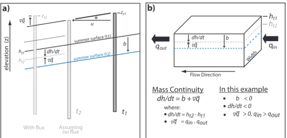
3. SCIENTIFIC BACKGROUND t1 t2 elevation (z) b dh/dt Assuming no flux With flux ht1 ht2 ht1 ht2 Flow Direction qin qout a) b) α u dh/dt Width b

summer surface (t1)

summer surface (t2)

dh/dt = b + q b < 0 dh/dt < 0 q > 0, qin > qout

Mass Continuity In this example

where: dh/dt = ht2 - ht1 q = qin - qout zt1 zt2 q Δ q Δ q Δ Δ Δ Δ

Figure 3.1: Schematic of mass continuity in the ablation area of a surface mass balance stake (a) and of a larger 3 dimensional cross sectional volume of a glacier (b). The surface elevation (h) and the top of the stake elevation (z) is shown for two discrete times (t1and

t2). bis the surface mass balance,uis the horizontal velocity, andαthe surface slope

of the surface between the stake position att1 andt2. The ﬂux divergence (∇q) is the

(17)

3.1 Mass continuity

divergence (∇q) is the column average velocity (eq. 3.4) multiplied by the density,ρ, which closely approximates the density of ice in cases where ﬁrn is a small proportion of the ice thickness (Cuﬀey and Paterson, 2010).

To relate the mass change (left side of eq. 3.2) to observed elevation changes (∂h_∂t), we introduce an eﬀective density (ρeﬀ) to express the vertical and temporal density changes of the column:

∂ ∂t _h_s hb ρ dz≈∂h ∂t·ρeﬀ (3.5)

It is also convenient to continue in water equivalent units because this is the common measuring practice for the glacier mass balance (b). We now assume that englacial and basal mass balances are negligible (be<< bsandbb<< bs) and that the ﬂux divergence (∇q) represents mass change of incompressible ice. The continuity expression can then be reduced to:

∂h

∂t ·κ= (bs+·∇q)·ρ −1

w (3.6)

whereρwis the density of water andκis a conversion factor from height diﬀerences to water equivalent changes:

κ=ρeﬀ ρw

(3.7) If ∂h_∂t is observed over a significantly long time period,κcan be approximated by the density ratio of ice to water (0.9) below the ELA. This because small changes in the less dense snow have little impact on the column average density and thus all changes will be of incompressible glacier ice. In the firn area, changes in the proportion of firn to the ice column can alterκdue to the compressibility of firn. Often, it is assumed that firn thickness and density are constant through time (”Sorge’s Law”, Bader, 1954) in which caseκ= 0.9.

Fig 3.1a shows an application of mass continuity using a stake in the ablation area as reference to measure the surface mass balance and∇q. The surface slope (α) between the stake positions att1andt2is required to adjust the change in stake elevation (∂z_∂t) due to downslope migration (see also Hagen et al., 2005):

∇q=∂z

∂t+u·tan(α) (3.8)

The vertical change in height of the top of the stake (dz

dt) and the horizontal velocity (u) can be measured by diﬀerential GNSS techniques. The slope of the surface (α)

(18)

3. SCIENTIFIC BACKGROUND

must be estimated from a DEM or GNSS proﬁle. Fig 3.1b demonstrates the same example as above over a cross sectional volume. The change in surface slope over the representative block is not considered here, however, slope changes may be signiﬁcant on glaciers that have drastically changed their geometry, as in cases of glacier surges.

Solving mass continuity over the entire glacier system requires integration of eq. 3.6 over the glacier surface area (A):

A ∂h ∂t·κ· dxdy= ∂V ∂t =B− A∇ q dxdyˆ (3.9)

All terms in water equivalent, this relates the volume change (∂V_∂t) to the flux divergence (∇qˆ) and the glacier-wide mass balance (B). Applying the divergence theorem to the last term in eq. 3.9 results in the relationship between the glacier-wide integrated flux and the water equivalent flux through a boundary (R):

A ∇q dxdyˆ = R q nˆ dr (3.10)

and substitution into eq. 3.9 results in: ∂V ∂t =B− R q nˆ dr (3.11)

wherenis the normal vector to the closed boundary (R). The second term on the right may represent the inﬂux of ice by avalanching or the loss through calving.

Using eq. 3.11, we consider two solutions: non-calving and calving glaciers. Often for non-calving glaciers,_R(q n)dris assumed equal to zero resulting in:

∂V

∂t =B (3.12)

This has formed the basis of many comparison studies aimed to control systematic errors in the cumulative direct surface mass balance integration by using geodetically measured volume changes (e.g. Krimmel, 1999; Elsberg et al., 2001; Cox and March, 2004; Thibert et al., 2008; Zemp et al., 2010, etc.). For a calving glacier,_R(q n)dris equal to the ﬂux (Q) through the boundary (R) of the glacier:

∂V

∂t =B+Q (3.13)

Practically solving mass continuity of an entire glacier system requires deﬁnition of the boundary geometry. For simplicity or due to lack of updated maps, this geometry

(19)

3.2 Glacier elevation changes

may be held constant. For example, Elsberg et al. (2001) introduce the concepts of a

reference and conventional surface for mass balance integration and suggest a trans-formation between them. Thereferencesurface is a constant map year and considered to be more climatically related as it removes the eﬀects of surface change on the mass balance. Theconventional mass balance is the actual mass change of the glacier rel-evant for hydrological and sea-level change studies. Equation 3.13 can be modiﬁed to handle the volume of retreat/advance separately:

∂Vr/a

∂t =Br/a+Qr/a (3.14)

where

Qr/a=Q−Q (3.15)

Derived in this way, ∂V_∂t and B of eq. 3.12 and 3.13 can be solved using areference

surface defined as the smallest glacier area. Q is then the ice flux through the cross sectional area (flux gate) defined by the glacier front at the time of smallest glacier area (i.e. the most recent area in cases of retreat). ∂V_∂tr/a, andBr/aare the volume change and mass balance of the receding (r) or advancing (a) area. ∂Vr/a

∂t is unproblematic to quantify provided knowledge of the basal elevation or depth below sea level in the retreat or advance area. Br/acan be solved by assuming a linear retreat of the front.

Qr/a is defined as the retreat/advance flux and is the difference between the net flux into or out of the glacier and the flux out of the gate defined by the front of the smallest area (Q). Hence,Qa>0 andQr<0.

3.2 Glacier elevation changes

With the increasing employment of satellite surface elevation measuring techniques, glacier volume change (as in equation 3.12, 3.13 and 3.14) becomes easier to monitor globally at higher spatial and temporal resolutions while the accuracy of modern tech-niques is also improving. The ability to measure glacier volume changes accurately is co-dependent on the magnitude of the glacier changes and the accuracy of the surface elevation measurements. This section provides a methodological background for de-riving elevation changes from remote sensing, an application that is present within all articles of this thesis.

(20)

3.2.1 Elevation Data

Elevation data can be acquired from the ground or from airborne and space-borne platforms. Ground and aerial techniques may provide the highest data accuracy and precision, however space-borne techniques provide a larger spatial coverage in less time at the potential cost of spatial resolution than the former acquisition platforms. In this thesis, surface elevations are acquired using phase-based differential GPS transported on the Earth’s surface (i.e. snow-mobile), by using RADAR (RAdio Detection And Ranging) and LIDAR (LIght Detection And Ranging) sensors at a significant distance from the target being observed or by photogrammetry using images of the same target from two or more observation points. All techniques are based upon remote sensing either utilizing the time (or phase) difference between sent and received signals or through solving the stereo parallax by the projected intersection of image path rays on the earth’s surface.

Stereo photogrammetry

Photogrammetric elevation data are typically in the form of a Digital Elevation Model1 (DEM), defined here as any elevation surface represented by a continuous collection of adjacent pixels that describes the mean elevation within every pixel. Measuring surface heights through photogrammetry relies on the principle of parallax which is the apparent shift in the position of an object due to a shift in the position of the observer (Mikhail et al., 2001). A parallax measurement is the difference between the stereo rays of the same target from each image projected onto the Earths ellipsoid and can be converted to height if the two observer positions and the focal length of the camera are known (Lillesand et al., 2004). The Base-To-Height (B/H) ratio is ana prioriestimate of parallax precision based upon the stereo geometry (Toutin, 2008). Image matching techniques (e.g. Debella-Gilo and Kääb, 2011) are used to automatically detect the same target in two or more images, a technique dependent upon the visible contrast of the targets and the pixel resolution of the images. Thus, the low visible contrast of the higher firn areas of glaciers remain a weakness of this elevation determination technique. Correlation masks from the image matching routines provides control on

1_{A diﬀerence exists between a digital elevation model (DEM), digital surface model (DSM) and}

digital terrain model (DTM). A DEM may be either a DSM or DTM, the former including vegetation and man made structures such as buildings and constructions. The latter containing the terrain alone.

(21)

determining the same target in both images. Further details about photogrammetric methods can be found in the plethora of books and manuals about photogrammetric techniques (e.g. Schenk, 1999; Mikhail et al., 2001; Lillesand et al., 2004; Kääb, 2005). Stereoscopic DEMs derived from airborne vertical frame images are used in all article of this thesis. In Article I, contour data made from an analogue photogrammetric workstation is used as the earliest map for elevation change comparison. This type of data contains limited accuracy and precision partly due to the dependence upon the individual photogrammetrist to locate the same target in the image pair. Article I also uses a digital photogrammetric DEM in which image matching techniques decrease the dependence of precision upon the photogrammetrist. In that study, elevation differences with ICESat over assumed stable terrain resulted in a 3 m RMSE for the digitally made DEM as compared to 12-15 m for the analogue data (Figure 1, Article I). The data used in Article IV also provided an interesting opportunity to directly compare analogue and digital methods applied upon the same images. Although not shown directly in that article, the standard deviation of differences between contour vertexes and the bilinear interpolation of the DEM was≈12 m for the glacier surface and≈22 m for the non-glacier terrain. This difference is partly a slope induced affect as the stable terrain surface contains steeper slopes than the glacier such that small horizontal distortions exaggerate vertical differences.

Two types of satellite stereoscopic DEMs are used in this thesis, both automatically generated without the use of ground control points (Fujisada et al., 2005; Bouillon et al., 2006). The ASTER instrument, on-board the Terra platform, contains stereo capability with a nadir and back-looking sensor (B/H ratio = 0.6) recording in the near-infrared part of the electromagnetic spectrum (ERSDAC, 2005; Toutin, 2008). Article III uses ASTER DEMs generated automatically from the SilcAst software downloaded from USGS LPDAAC (Land Process Distributed Active Archive Center) which provides a 30m pixel resolution product. Articles II, III and IV additionally use automatically generated DEMs from the SPOT5-HRS stereo sensors (B/H ratio = 0.8) acquiring ≈5 m panchromatic images resulting in 40 m DEM products (Bouillon et al., 2006; Korona et al., 2009).

The errors within stereoscopic DEMs can be classiﬁed as blunders, stochastic and systematic errors. Figure 3.2 shows examples of the three error types in ASTER stereo-scopic DEMs. Blunders are errors that derive from image matching failure and are

(22)

4

10 Km 10 m -10 m 0 10 20 30 40 50 60 -2 -1 0 1 2 Dist ance ( km ) Vertical Di_erences

a)

b)

Franz Joseph Glacier

Figure 3.2:Examples of the stereoscopic error types. (a) is a hillshade from an ASTER SilcAst DEM (7 April 2001: L1A.003:2007486672) over Franz Joseph Glacier in New Zealand and the associated orthophoto (inset). The blue ellipse is an example of a blunder that appears as an artificial mountain/hill. The yellow ellipse shows the stochastic errors in the DEM when visible contrast is limited which appear as rough (”bumpy”) surfaces in the hillshade. (b) shows the elevation differences between 2 ASTER SilcAst DEMs from 2002 and 2006 in the same region of New Zealand after co-registration and removal of a longer frequency elevation bias (see Article III for further details). The white lined plot shows the across-track elevation difference averages that exhibit a sinusoidal pattern along track that is related to satellitejitter, high frequency shaking of the instrument, that is not captured by the under-sampled satellite attitude measurements (Leprince et al., 2007).

(23)

strongly autocorrelated in space. They can typically occur in areas of similar looking contrast from either topography or clouds, on ice caps or lakes. Blunders will typically appear as large holes in the DEM, or as additional mountains. Stochastic errors are the random errors that mostly derive from the image matching process and will vary for diﬀerent image resolutions, visible contrast conditions and pyramidal processing methodology. Systematic errors are generally in the form of translations, tilts, rota-tions and in the worst case, scale distorrota-tions. Systematic errors will also vary based upon the acquisition strategy, ie. whether frame imagery or pushbroom sensors are be-ing used to collect the data. Article III provides a detailed description of how to detect, and suggestions for correcting, errors related to the geolocation of the original data, elevation dependent scale errors and along/across track biases, all of which are system-atic errors that can commonly exist within pushbroom derived satellite stereoscopic DEMs.

LIght Detection And Ranging (LIDAR)

The principle behind LIDAR techniques is to measure the time it takes a transmitted pulse (signal) to be sent to an object, reﬂected, and returned to the receiver. This active remote sensing technique can be applied using sensors operated from the ground (terrestrial), carried by planes (aerial) and from space (satellite). The former two plat-forms for LIDAR acquisition are not used in this thesis, though the immensely improved accuracy and details contained within LIDAR DEMs has increased the applicability of these data sets to many ﬁelds within geoscience (Blair et al., 1999; Drake et al., 2002; Hopkinson and Demuth, 2006; James et al., 2006; Barrand et al., 2009; Abermann et al., 2010).

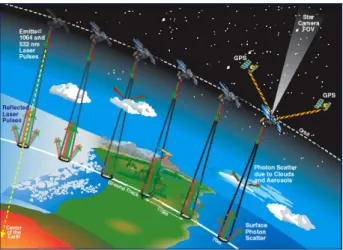
The LIDAR data used in this thesis is acquired from a satellite platform. The Ice, Cloud and land Elevation Satellite (ICESat) carrying the Geoscience Laser Altimeter System (GLAS) was launched in 2003. The acquisition strategy was reduced because of the abrupt failure of the ﬁrst of three lasers. However, the mission surpassed the initial goal of a three year campaign by two years and it acquired nearly 2 billion elevation points before failure of the ﬁnal laser in October 2009 (http://icesat.gsfc.nasa.gov). ICESat contained three lasers, each with two telescopes one infra-red (1024 nanome-ters) and one visible green (532 nanomenanome-ters) for the land surface and atmosphere, respectively. The laser pulses at 40 Hz which translates into a seperation distance on

(24)

Figure 3.3: Schematic example of ICESat measurmenets of the earth’s surface. cNASA (Graphic created by Deborah McLean).

earth’s surface of≈170 m between each footprint (see schematic illustration, Fig. 3.3). ICESat averaged 2-3 acquisitions per year repeating similar reference tracks within a few hundred meters in the arctic. The amount of data is also much higher in the arctic as compared to the equator due to the polar orbiting strategy of the satellite. Full details of the ICESat mission can be found in Zwally et al. (2002b) and Schutz et al. (2005).

The GLAS instrument onboard ICESat is designed to measure the precise time it takes the laser pulse to travel from the satellite to the earth’s surface and back again. The transmitted laser pulse is reflected from an elliptical footprint of the earth’s surface that varied from 52X95m (lasers L1-L2c) to 47x61m (lasers L3a and L3b), an average of 64m (Abshire et al., 2005). For each transmitted laser pulse, the altimeter collects 4.5 million 1 nanosecond samples that is pre-processed onboard into 544 samples for transmission back to earth. To determine in which 544 sample time range the reflection from the earth’s surface is contained, a generalized DEM is used to predict the time return (Brenner et al., 2003). Elevations are obtained by fitting Gaussian functions to the returned waveforms where the maximum amplitude of the return marks the two-way travel time which translates into distance from the satellite.

(25)

el-3.2 Glacier elevation changes 1 Km 1 - 100 101 - 200 201 - 300 301 - 400 401 - 977 Waveform Width (nanoseconds)

Dahlbr

een

80°N 78°N 25°E 15°E 0 100 200 300 400 500 600 -20 0 20 40 60 80 100 0 100 200 300 400 500 600 -20 0 20 40 60 80 100 0 100 200 300 400 500 600 -50 0 50 100 150 200 Time (ns) [1 ns = 0.15 m]

Return echo pulse c

ount

a)

b)

c)

d)

b)

c)

d)

width

Figure 3.4: Examples of returned ICESat waveforms on varying glacier surfaces. (a) shows ICESat footprints from September 2003 that are color coded to a classiﬁcation of return waveform widths. The background is a 2007 SPOT-HRS orthophoto. The exact crevasse pattern in the image may not correspond to the 2003 ICESat waveforms. The waveforms located in the crevasse zone (b and c) are wider than that located in a smoother glacier surface region (d). The width of the waveform represents the range of elevation from which the laser pulse is reﬂected, inferring crevasse depths of≈30 meters.

(26)

evation (Brenner et al., 2003). The shape of the returned waveform is wider based upon the distribution of elevation within the reﬂected footprint. Therefore, slope broadens the waveform because of the larger range of elevation within a footprint and roughness increases the width because of the more uniform distribution of elevation within a foot-print. Thus, only slope assuming no roughness or roughness assuming no slope may be extracted from the waveform (Brenner et al., 2003). Figure 3.4 shows an example of waveform widths on the tongue of a calving glacier in western Spitsbergen.

ICESat data is freely available, distributed by the National Snow and Ice Data Center (NSIDC; www.nsidc.org). In this thesis, two 2nd level products are used, GLA06 (Zwally et al., 2010a) and GLA14 (Zwally et al., 2010b). The products differ by the number of potential Gaussian fits used to determine the mean elevation within the footprint. The GLA06 products are meant for glaciers and ice sheets because their relatively flat surfaces typically return waveforms that approximate a single gaussian and thus the average centroid of maximum two Gaussian fits are used to determine the mean elevation within the footprint. The GLA14 products are designed for land terrain surfaces as the steeper slopes, greater roughnesses and possible vegetation produce wider and multi-model echo waveforms. Therefore, GLA14 uses an average of maximum six Gaussian fits to determine the mean elevation within the reflected footprint (Zwally et al., 2002b). The difference between the two products is small, with average differences less than about 20 cm, standard deviations of≈60 cm though maximum differences up to±3 m in the alpine terrain of New Zealand and Svalbard (Figure 3.5).

The previous example shows that random errors (precision) associated with the Gaussian fitting method in the GLA06 and GLA14 products is≈0.6 m in alpine terrain, which is equal in magnitude to the width of the transmitted laser pulse. Fricker et al. (2005) assessed the performance of the GLAS altimeters in optimal conditions (similar to an ice sheet) by comparison to an extremely precise DEM from dGPS kinematic profiles on the bright salt flats of salar de Uyuni, Bolivia (Borsa et al., 2008). They find an absolute accuracy (bias) of<2 cm and precision (σ)<3 cm though significant degradation was found on saturated returns which contained an increased bias (-1 m). In this thesis, ICESat releases newer than 28 have been used and thus saturation range corrections have been applied. In addition to saturated returns, Fricker et al. (2005) describes waveform returns in which atmospheric forward scattering of photons was present (e.g. within a thick cirrus cloud layer or from blowing snow) producing

(27)

Stable Terrain (Land)

Ice/Snow (Glacier)

Elevation Difference (m)

[GLA06 minus GLA14] Mean = 0.16 St. dev = 0.66 n = 33824 Mean = 0.21 St. dev = 0.43 n = 54485

S

valbar

d

New Z

ealand

-3 -2 -1 0 1 2 3 0 1000 2000 3000 4000 5000 6000 -3 -2 -1 0 1 2 3 0 10 20 30 40 50 60 70 -3 -2 -1 0 1 2 3 0 500 1000 1500 2000 2500 3000 -3 -2 -1 0 1 2 3 0 500 1000 1500 2000 2500 3000 3500 4000 Mean = -0.07 St. dev = 0.63 n = 44173 Mean = -0.05 St. dev = 0.93 n = 588

Figure 3.5: Histograms of the elevation diﬀerences between GLA06 and GLA14 ICESat products on stable terrain and over ice. The two datasets, Svalbard and New Zealand, are those used in Articles I, II, and III and are from the most recent release, 31. A larger dataset of glacier ice/snow comparisons are available in Svalbard, and many of those on stable terrain may be snow covered. The two distributions on Svalbard also seem slightly skewed towards more positive GLA06 elevations than GLA14 elevations. This is most likely the lack of saturation corrections in the GLA14 products since super-saturated signals generally result in a longer range, thus lower elevation of the GLA14 products (Fricker et al., 2005).

(28)

elongated tales on the waveforms (Duda et al., 2001) and increasing both the bias (-16 cm) and σ (8 cm). Accuracy can also be assessed by the cross over or intersection points of ascending and descending tracks over the ice sheets and ice caps. On surface slopes less than 1.15 degrees, the precision (σ) of ICESat crossovers were better than 0.5 meters (Brenner et al., 2007) and on slopes less then 5 degrees,σwas better than 0.7 m (Moholdt, 2010). In Antarctica, crossovers of laser 2a showed accuracies of≈0.2-0.3 (2 m in worst case) and precisions of≈0.25 m (Shuman et al., 2006). Combining this with the Fricker et al. (2005) precision estimates and those from the Gaussian ﬁtting between GLA06 and GLA14 (Fig. 3.5) results in an average accuracy and precision of better than a meter. This estimate is however mainly based on the idealized case of low sloping glacier surfaces. The footprint of the laser increases in area over steep terrain and thus the wider waveform degrades elevation estimation. In addition, the laser does not penetrate thick clouds which can signiﬁcantly reduce the amount of data.

RAdio Detection And Ranging (RADAR)

Measuring earth’s surface using RADAR is accomplished by two techniques, radar pulse altimetry (similar to the LIDAR techniques described above) and radar interferometry. Only the nearly-global interferometric DEM from the Shuttle Radar Altimetry Mission (SRTM) is used in this thesis (Article III). SRTM launched an interferometric radar with two antennas attached to the space shuttle, Endeavor, in February 2000, and over the coarse of 11 days mapped ≈80% of the earth’s surface (from 60o N to 56o S) (Farr et al., 2007). SAR interferometry uses the phase diﬀerences between two radar images acquired with a small base-to-height ratio (e.g. STRM has a baseline of 60m). These phase diﬀerences are the photogrammetric equivalent to a parallax measurement allowing retrieval of topography (Rosen et al., 2000). Typically reported vertical accuracies of the dataset are 10m which is lower than the mission standards of 16m (Rodriguez et al., 2006). However, vertical biases are present due to instability of the sensor and/or platform (Rabus et al., 2003), and biases have also been shown due to penetration of the C-band Radar waves into snow/ice (Rignot et al., 2001; Berthier et al., 2006).

(29)

3.2.2 Methods of comparison

From the two data types of point elevation measurements and semi-continuous DEMs, this thesis calculates elevation changes using three approaches:

[1] Extract the underlying DEM elevation to a point using a bilinear interpolation of the 4 nearest pixels. Other interpolation methods can be used, however, a nearest neighbor interpolation scheme induce horizontal shifts between the data products.

[2] Calculate repeat ICESat track elevation diﬀerences after correcting or solving for the across track slope between near-repeat tracks.

[3] Diﬀerence two continuous DEMs pixel by pixel. Re-sampling is often required and interpolation methods more advanced than a nearest neighbor should be used. Bilinear interpolation is used in all research presented here.

Method [1] is applied for any comparisons between ICESat and a DEM (Article I and III). Three methods for comparing ICESat tracks to contour lines were examined in Article I. The most precise method was the bilinear interpolation of the intersection point between an ICESat track and a contour line. However, intersections are limited on the ﬂat glacier surfaces and the increased sampling by comparing the bilinear in-terpolation of ICESat into a contour interpolated DEM (Method [1]) generated a more statistically and spatially robust estimate. Mean glacier elevation changes did not show large variability between the three methods when estimated over larger spatial regions (Table 3 in Article I).

Method [2] is developed within the PhD thesis of G. Moholdt (2010) and applied in Article II to generate a 5 year elevation change estimate over the glaciers and glacier regions of Svalbard. The approach is developed for the rather small across-track spacing of the ICESat repeat tracks common in the polar regions (<200 m). It is based upon fitting planer surfaces to a set of at least 5 repeat tracks within 700 m windows using a multiple linear regression. The multiple linear regression solves for the surface slope and the linear average elevation change rate of all points that fall within that plane. The configuration of the repeat tracks in time and space is crucial for this method; for example, (1) if the two tracks furthest from the central track were in opposite seasons, the plane fitting compensates in the slope estimate leading to biased elevation change

(30)

estimates, and (2) inclusion of varying start and end season data in the population of planes over-samples either winter or summer which results in biased estimates of elevation changes. To verify the ICESat independent elevation change measurements, two additional approaches were applied; (1) cross-over (intersection) points and (2) along DEM-projected repeat tracks. Cross-over measurements are the most accurate, however, the amount and distribution of them were far too limited to estimate volume change. Using a DEM to re-project repeat tracks provides enough measurements but the precision of them was slightly less than the ICESat independent approach (method [2]) which does not require an external DEM.

Procedures for DEM differencing (Method [3]) are described in great length within Article III and applied in Article IV. The sub-pixel geolocation accuracies of the DEMs available depends strongly upon the acquisition of the data (aerial or satellite) and the formation of the photogrammetric model block. The geolocation of the satellite DEMs used in this thesis are strictly dependent on the on-board location and attitude measurements that are used to intersect the pixels onto earth’s ellipsoid. Aerial pho-togrammetric DEMs are dependent upon the CGPs that form the stereoscopic model block. Therefore, comparison of the two (if both are not aerial DEMs constructed us-ing the same GCPs) requires co-registration. In Article III, an analytic method based upon slope and aspect (Kääb, 2005) is programmed and applied universally to check and correct for horizontal and vertical shifts. After co-registration, elevation-dependent and along/cross track biases are checked and removed before performing the final dif-ferencing.

3.2.3 Determination of volume changes

Two methods for estimating the total volume change of a glacier or glacier region from elevation changes exist. Ideally, two DEMs are available such that pixel by pixel eleva-tion changes can be summed over the glacier or glacier area of interest (nA, equivalent to the number of glacier pixels) and multiplied by the pixel area (r2_{) to estimate the} volume change (Etzelm¨uller, 2000):

dV dt = nA 1 dh dt·r 2 _(3.16)

This method will be referred to as thegrid method. When continuous DEMs are not available, often ahypsometric approach is applied by deriving an elevation change by

(31)

elevation relationship, dh

dt(z), and multiplying by the hypsometric distribution of the glacier,A(z): dV dt = z 1 [dh dt(z)·A(z)] (3.17)

Equation 3.17 requires the assumption that the distribution of elevation changes within an elevation bin is normally distributed around the mean estimate derived along the centerline or averaged over an elevation bin (Berthier et al., 2004). The application of eq. 3.17 is most common in cases of centerline altimetric data (Arendt et al., 2002) but can also apply in cases where data is randomly distributed (Article I and II) or when missing data (i.e. holes in the DEM) render eq. 3.16 unsolvable over the entire glacier (Article IV).

3.2.4 Assumptions

The major assumption in studies of elevation and volume change is the conversion into mass or water equivalent changes1_{. The common approach is to assume Sorge’s Law} based upon Earnest Sorge’s observation in the dry snow zone (no melting) at Eismitte, Greenland (1930-1931) that ”the density of snow at a given depth below the surface does not change with time” given a constant accumulation rate (Bader, 1954). This also implies that the age of a particular snow layer at depth remains constant (Bader, 1954), and therefore the thickness of the firn layer constant. It is still unclear whether densification processes affect the interpretation of glacier elevation changes and what are the dominant factors affecting firn densification rates (Li et al., 2007; Reeh, 2008; Arthern et al., 2010). Nonetheless, Sorge’s Law defines the assumption of a constant firn layer thickness and density, and therefore is the justification of assuming ∂h

∂t and ∂V

∂t are composed solely of ice.

Very few, if any, dry snow zones exist on Svalbard which brings into question the validity of Sorge’s Law since it is based upon observations where there is no percolation. Even at some of the highest elevations in Svalbard, percolation persists practically ev-ery year (see e.g. Pohjola et al., 2002b) and thick ice layers and lenses are commonly found within the ﬁrn zone (Hawley et al., 2008; Langley et al., 2009). If the amount of

1_{Strong erosional forces of a glacier may also change the measured height of the surface, however}

this process (and the magnitude of) operates on a time-scale much longer than the measurements, and thus are assumed negligible.

(32)

percolation that occurs within each year is normally distributed through time (annu-ally), then Sorge’s Law most likely holds. On one of the highest glaciers in Svalbard, Holtedahlfonna, multiple ice cores with a time separation of 13 years (Uchida et al., 1993; Sjögren et al., 2007) showed a randomly varying density of the upper most firn layers, but the boundary transition to continuous glacier ice occurred at practically the same depth in both cores providing assurance that the firn thickness and density has not changed drastically within this time period (Fig. 7, Article I).

Another bias introduced by using the density of ice for conversion is if the ELA has migrated within the time epoch and firn is either gained or lost. For example, on Austfonna in the period 2003-2007, the spatial area of the firn zone increased (Dunse et al., 2009) warranting a lower density conversion factor (Moholdt et al., 2010a). Some studies have also determined the reduction in the density conversion factors using the estimated percent area of firn/ice change (Sapiano et al., 1998). Other approaches to account for this uncertainty are to apply the density of firn above the ELA and the density of ice below (Hagg et al., 2004) or an elevation dependent function of density (Article II). In summary, the uncertainty in mass conversion (density) reduces the accuracy of geodetic estimates and the effect of the bias has been estimated to be up to 5-6% of the volume change (Elsberg et al., 2001; Cuffey and Paterson, 2010), of course depending on the magnitude of the measured changes.

3.3 Glacier Surface Mass Balance

The surface mass balance of a glacier is deﬁned as the sum of mass gain by accumula-tion and loss through melt water runoﬀ. It represents the interacaccumula-tion between glacier and atmosphere and is the climatic driver of the glacier system. The mass balance is typically seasonal (except for low-latitude and tropical glaciers) in which accumulation falls in the winter and melting occurs in the summer. Both of these components contain gradients with elevation notably due to the general decrease of temperature with in-creasing elevation. Accumulation typically increases with elevation because the colder atmosphere holds less water thus more precipitation. Melt decreases with elevation due to the warmer temperatures lower. A given point lower on the glacier therefore experiences a longer ablation season with larger melt amplitudes than higher up that experience a longer accumulation season with larger snow depths. Glacier surface

(33)

3.3 Glacier Surface Mass Balance

mass balance can be observed directly by measuring the amount of water equivalent snowfall and melt in discrete temporal and spatial steps. Determining a continuous surface mass balance ﬁeld remains nearly impossible, thus interpolation and extrapo-lation procedures are often required. Conveniently, the dominant parameter used for interpolation and extrapolation is elevation due to the good correlation to surface mass balance.

3.3.1 Direct mass balance observations

This section describes the surface mass balance as measured on Holtedahlfonna used for Article IV. Direct surface mass balance measurements are acquired using 6 m stakes drilled into the ice/ﬁrn, commonly aligned along the centerline of glaciers (e.g. Hagen et al., 1999) with enough stakes to capture the elevation variation of mass balance. As few as 5 stakes are required when the transverse mass balance variability is small (Fountain and Vecchia, 1999). Other glaciers contain immense stake networks that cap-ture both elevation and lateral dependence of the surface mass balance (e.g. Krimmel, 1999; Jansson and Pettersson, 2007).

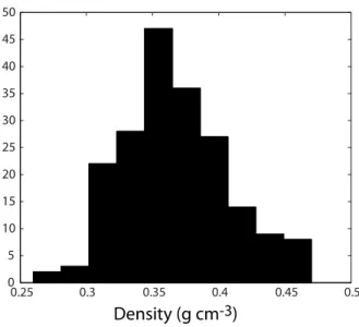
To measure the surface mass balance from a stake, the change in exposed stake length is measured on an annual or seasonal basis where the difference in height mul-tiplied by the density of the material gained/lost returns the specific mass balance. In winter, snow density is measured traditionally using snow pits and/or ice cores. A collection of 196 snow pit bulk density measurements made between 2000 and 2009 on glaciers in northwest Svalbard (around Ny ˚Alesund) have a mean bulk density of 0.37 g cm−3_{with a standard deviation of 0.04 g cm}−3_{(Figure 3.6, J. Kohler, unpublished).} For winter measurements, the bulk density is used to convert the stake length changes into water equivalent. For summer measurements in the ablation area, the density of the snow pack is used to convert the exposed stake length change up to the winter snow pack thickness and the density of ice (0.9 g cm−3_{) is used for conversion of all} residual change in exposed stake length. If the exposed stake length is increasing in the firn area, the density of firn is required to convert to mass changes, assuming negligible internal accumulation. Common firn densities are quoted between 0.4 and 0.8 g cm−3 (Paterson, 1994) and firn density profiles with depth are available from the various ice cores around Svalbard (e.g, Uchida et al., 1993; Pinglot et al., 1999; Isaksson et al., 2001; Pohjola et al., 2002a; Sjögren et al., 2007). Figure 3.7 shows the 7 year series of

(34)

3. SCIENTIFIC BACKGROUND 0.25 0.3 0.35 0.4 0.45 0.5 0 5 10 15 20 25 30 35 40 45 50

Density (g cm

-3

₎

Figure 3.6: Histogram of 196 snow pack bulk densities over the period 2000 to 2009. The measurements are made on 3-4 glaciers in the Ny ˚Alesund area, and the number of pits varies for each year. The average bulk density of the winter snow pack is≈0.37 g cm−3. (Provided by J Kohler, Norwegian Polar Institute).

(35)

3.3 Glacier Surface Mass Balance 0 500 1000 1500 -200 -100 0 100 200 2003 0 500 1000 1500 -200 -100 0 100 200 2004 0 500 1000 1500 -200 -100 0 100 200 2005 0 500 1000 1500 -200 -100 0 100 200 2006

M

ass Balanc

e (cm)

0 500 1000 1500 -200 -100 0 100 200 2007 0 500 1000 1500 -400 -200 0 200 2008 0 500 1000 1500 -300 -200 -100 0 100 200 2009 0 500 1000 1500 -400 -200 0 200 2010

Elevation

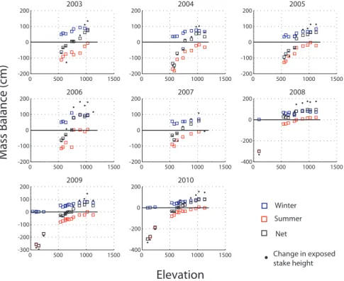
Winter Summer Net Change in exposed stake height

Figure 3.7: Change in exposed stake length and water equivalent conversions of the winter, summer and net surface mass balances plotted against elevation for the 2003-2010 time series on Holtedahlfonna and 2008-2003-2010 time series on Kronebreen. The stake measurements are used to calibrate a surface mass balance model in Article IV.

stake measurements on Holtedahlfonna. The original change in exposed stake length is shown as dots. Squares are the surface mass balance estimates after conversion into water equivalent using densities of 0.37, 0.55 and 0.9 g cm−3 _{for snow, ﬁrn and ice,} respectively.

To determine the glacier wide surface mass balance (B), the discrete speciﬁc mass balance measurements are extrapolated over the entire glacier surface utilizing the dependency with elevation (similar to equation 3.17):

B= z

1

(36)

where b(z) is the winter, summer and/or net surface mass balance as a function of elevation or average within an elevation bin, andA(z) is the hypsometry. The function of elevation may be solved as either a linear, piece-wise linear, or polynomial (Foun-tain and Vecchia, 1999). On glaciers with with a dense spatial distribution of speciﬁc point measurements, kriging has been applied (Hock and Jensen, 1999; Jansson and Pettersson, 2007). Typically the hypsometry for each individual mass balance year is not available. Therefore, if hypsometries at the start and end year of the mass balance time series are available, then a temporal interpolation can be applied assuming a linear transformation between the two map products (Cox and March, 2004; Thibert et al., 2008). If only one hypsometry is available, a reference surface mass balance can be estimated (Elsberg et al., 2001).

The errors associated with surface mass balance measurements include measurement errors, density conversion errors and sampling errors. Jansson (1999) finds that the surface mass balance of Storglaciären is not sensitive to density and sampling error and thus using only a sparse distribution of stakes results in a stochastic error of≈ ±0.1 m. Other studies have suggested errors of the specific measurements between 0.2 and 0.4 m (Lliboutry, 1974; Cogley and Adams, 1998; Cox and March, 2004) and even larger errors are derived by combining all stochastic and potential systematic errors (Thibert et al., 2008; Zemp et al., 2010). Systematic errors are difficult to detect and may derive from sinking stakes in the firn area (Østrem and Brugman, 1991), or from unaccounted superimposed ice and/or internal accumulation (Thibert et al., 2008; Zemp et al., 2010). Lastly, accumulation of errors can be common when summing annual mass balance measurements to derive a cumulative mass balance time series (Conway et al., 1999; Krimmel, 1999; Andreassen, 1999; Thibert et al., 2008).

3.3.2 Mass balance modelling

An alternative to using the raw speciﬁc mass balance measurements for extrapolation over the entire glacier is to use the measurements for calibrating a mass balance model that functions as a spatial and temporal interpolator/extrapolator. For the winter accumulation, if only a single season model is required, the snow depth at the end of winter can be used as initial input (Arnold et al., 2006; Schuler et al., 2007). For multi-annual applications, accumulation can be approximated by correlation to local measurement stations or by downscaling precipitation in regional climate models (e.g.

(37)

Barstad and Smith, 2005; Schuler et al., 2008; Rye et al., 2010). For ablation mod-elling, two approaches exist; the physically based energy balance approach and the empirical temperature-index model (Hock, 2005). Studies that have applied and com-pared both models on the same glacier suggest that the physical energy balance is more accurate and correct on models aiming to capture the daily variability of melt while empirical approaches perform equally well when experimenting with long time series (Gudmundsson et al., 2009; Pellicciotti et al., 2005)

The physically based melt modelling approach aims to solve the surface energy balance from measured (or simulated) radiation, temperature, humidity and wind to determine the turbulent fluxes and an estimate of the available energy for melt (Hock, 2005). However, the spatial distribution of the energy balance model is difficult as measurements of all the above parameters are not possible over the entire glacier, and thus estimates or simulations of the radiation fields and the evolution of albedo are required for proper distribution (e.g. Arnold et al., 1996; Brock et al., 2000; Dadic et al., 2008). Nevertheless, incorporation of satellite data sets such as MODIS may help constrain albedo in models operating within the lifetime of such satellites.

Empirical approaches can also be used to model the surface mass balance, provided proper calibration and constrain by melt measurements. The classical degree day ap-proach relates melt solely to temperature while advanced degree day models include parameterizations for solar radiation (Hock, 1999; Pellicciotti et al., 2005). In Article IV, both empirical models were tested though a classical degree day approach was cho-sen due to equiﬁnality of the calibrated parameter sets in the advanced model (lack of model constrain1_{). In the classical degree day approach, melt is assumed to vary} linearly with temperature only if the temperature (T) is above some temperature-melt threshold (T0):

Melt=DDFsnow_/ ice

_·₍_T₋_T₀₎ _(3.19)

Degree Day Factors (DDF) are typically determined through statistical methods of minimizing the residuals between modelled and measured values (e.g. Hock, 1999). The degree day factors vary for snow and ice due to the varying albedo of the surfaces (Braithwaite, 1995). This implies that theDDFsnow should be lower than DDF_ice

1_{All stake measurements used to calibrate and constrain the models are located along the centerline}

(38)

3. SCIENTIFIC BACKGROUND 0 100 200 300 400 500 600 700 800 900 1000 −1000 −500 0 500 1000 1500 2000 2500 3000

Positive Degree Days

Summer Mass Balance (mm)

Kongsvegen Kronebreen Tmean T0 = 0 Tmean T0 = -5 Tmean T0 = -2 Tmax T0 = 0

Figure 3.8: Positive Degree Days estimated for each annual stake measurement on Kongsvegen and Kronebreen, presented in Article IV. For each glacier, 4 parameter set combinations are shown; [1,2,3]T= daily average temperature (Tmean) andT0= 0,-2 and

(39)

because the albedo of snow is higher than that of ice. Determining the threshold tem-perature for melt (T0) has important repercussions on the calibratedDDFs. Van den Broeke et al. (2010) showed that setting T0 to 0o C when driving the model with the daily average temperature (T) resulted in DDFsnow > DDFice, which is not reasonable. The cause is the temporal under-sampling as melting conditions may be experienced within the daily time step even if the daily average temperature is below T0. The under-sampling misses many potential melt days in the spring and autumn, andDDFsnow must increase to generate the amount of melt within a smaller summer time window (Van den Broeke et al., 2010). Figure 3.8 shows that varyingT0stretches the positive degree day scale (i.e.increases the range). Alternately, settingT equal to the daily maximum temperature andT0 to 0oC results in the same aﬀect as settingT to the daily average temperature andT0=-2oC.

(40)