Simulation of regional-scale water and energy budgets: Representation of subgrid cloud and precipitation processes within RegCM

Simulation of regional-scale water and energy budgets:

Representation of subgrid cloud and precipitation processes

within RegCM

Jeremy S. Pal

Department of Civil and Environmental Engineering, Ralph M. Parsons Laboratory for Hydrodynamics and Water Resources, Massachusetts Institute of Technology, Cambridge

Eric E. Small

Department of Earth and Environmental Science, New Mexico Tech, Socorro

Elfatih A. B. Eltahir

Department of Civil and Environmental Engineering, Ralph M. Parsons Laboratory for Hydrodynamics and Water Resources, Massachusetts Institute of Technology, Cambridge

Abstract.

A new large-scale cloud and precipitation scheme, which accounts for the

sub-grid-scale variability of clouds, is coupled to NCAR’s Regional Climate Model (RegCM).

This scheme partitions each grid cell into a cloudy and noncloudy fraction related to the

average grid cell relative humidity. Precipitation occurs, according to a specified

autoconversion rate, when a cloud water threshold is exceeded. The specification of this

threshold is based on empirical in-cloud observations of cloud liquid water amounts.

Included in the scheme are simple formulations for raindrop accretion and evaporation.

The results from RegCM using the new scheme, tested over North America, show

significant improvements when compared to the old version. The outgoing longwave

radiation, albedo, cloud water path, incident surface shortwave radiation, net surface

radiation, and surface temperature fields display reasonable agreement with the

observations from satellite and surface station data. Furthermore, the new model is able

to better represent extreme precipitation events such as the Midwest flooding observed in

the summer of 1993. Overall, RegCM with the new scheme provides for a more accurate

representation of atmospheric and surface energy and water balances, including both the

mean conditions and the variability at daily to interannual scales. The latter suggests that

the new scheme improves the model’s sensitivity, which is critical for both climate change

and process studies.

1. Introduction

In many applications of the National Center for Atmo-spheric Research (NCAR) Regional Climate Model (RegCM), an accurate simulation of the energy and water cycles is crucial [Giorgi and Mearns, 1999]. The presence of clouds and result-ing precipitation is the primary control on these cycles. It is therefore important to accurately represent cloud processes in many modeling applications. Clouds, however, are often poorly represented in both regional and global climate models (RCMs and GCMs, respectively) partly because some of the key cloud processes occur at spatial and temporal scales not resolved by current models. This study presents a simple, yet physical, resolvable-scale (nonconvective) moist physics and cloud scheme for the NCAR RegCM that accounts for the subgrid variability of clouds, the accretion of cloud water, and the evaporation of raindrops.

The response of the climate system to changes in greenhouse gases, sulfate aerosols, soil moisture, and vegetation is strongly influenced by cloud processes. For example, theIPCC[1995]

report on climate change indicates that the representation of cloud characteristics accounts for a large portion of the uncer-tainty in climate change predictions. They further indicate that inclusion of different cloud representations could result in dramatic effects as much as to double the expected 2.5⬚C warming or to reduce it by half. As another example,Pal and Eltahir[2000] suggest that cloud processes play an important role in determining the strength of the soil moisture-rainfall feedback. They show that a strong response of clouds to changes in soil moisture can nearly negate the soil moisture-rainfall feedback. The representation of clouds is also impor-tant for simulations of other land surface changes, including deforestation [e.g.,Eltahir and Bras, 1994], desertification [e.g., Xue, 1996], and desiccation of inland water bodies [e.g.,Small et al., 1999b].

The United States Midwest is one of the largest agricultural regions in the world. The crop yield during the growing season depends on a variety of factors, including the surface energy and water budgets. Predicting these budgets can be extremely useful for cropping strategies [Mearns et al., 1997]. However, to properly predict these budgets, it is mandatory to accurately represent clouds and precipitation. These energy and water budgets are also crucial in predicting flood and drought.

Forecasting flood and drought can be useful for a variety of Copyright 2000 by the American Geophysical Union.

Paper number 2000JD900415. 0148-0227/00/2000JD900415$09.00

purposes, including water resources management, cropping strategies, and saving human lives. For example, in 1988 the United States experienced its warmest and driest summer since 1936 [Ropelewski, 1988]. It resulted in⬃10,000 deaths from heat stress and caused an estimated $30 billion in agricultural damage [Trenberth and Branstator, 1992]. In contrast, during the summer of 1993, record high rainfall occurred over much of the midwestern United States causing persistent and devas-tating flooding throughout the upper Mississippi River basin [Kunkel et al., 1994]. The National Oceanic and Atmospheric Administration (NOAA) estimated that the flood caused $15–20 billion in damages (NOAA, 1993). It is shown in this paper that an adequate representation of clouds and precipi-tation is required to accurately predict flood and drought.

In the old version of RegCM (SIMEX moist physics [Giorgi et al. [1999]), the representation of land surface, radiation, and boundary layer processes (among others) is quite elaborate [Giorgi and Mearns, 1999]. However, the representation of cloud processes is not nearly so sophisticated. It is shown in this study that over North America the old version of RegCM tends to be too cloudy at times when clouds exist and not cloudy enough when clouds are not present. As a result, the seasonal variability of clouds tends to be overestimated. RegCM with the old moist physics scheme seems to neglect key processes required to accurately predict the observed variabil-ity of clouds.

To accurately simulate precipitation, one needs to account for various processes, including those that occur at scales finer than the model resolution. In the atmosphere, clouds often form over part of an area comparable to the size of a model grid cell when the area-average humidity is below 100%. Thus fractional cloud coverage varies between zero and 100% over the same area.Molinari and Dudek[1986] investigate a rainfall event that occurred over the northeastern portion of the United States using a RCM. They indicate that neglecting the subgrid variability delays the onset of precipitation. The col-lection of cloud droplets from raindrops falling through clouds and the evaporation of falling raindrops can be very important processes [Rogers and Yau, 1989]. Not including the former can lead to an underestimate of precipitation intensity and volume particularly over cloudy regions. Not including the latter can lead to an overestimate of precipitation particularly over arid regions [Small et al., 1999a] and can result in unrealistic model instabilities [Molinari and Dudek, 1986]. The old moist physics scheme neglects the above subgrid processes, while our new scheme accounts for these processes based on the work of Sundqvist et al. [1989] and others.

Section 2 provides a description of the old and new large-scale cloud and precipitation schemes, in addition to a brief description of RegCM. Section 3 describes the setup of the numerical experiments. The data sets used to evaluate the model performance are presented in section 4. The results and conclusions are provided in sections 5 and 6, respectively.

2. Description of Numerical Model

In this study we use a modified version of the NCAR RegCM. This section provides a general description of this model, in addition to a more detailed description of both the new and the old large-scale cloud and precipitation schemes.

2.1. General Model Description

The NCAR RegCM was originally developed byDickinson et al. [1989],Giorgi and Bates[1989], andGiorgi[1990] using

the Penn State/NCAR Mesoscale Model version 4 (MM4) [Anthes et al., 1987] as the dynamical framework. Here we provide only a brief description of RegCM (except for the large-scale cloud and precipitation models); A more detailed description can be found in the works ofGiorgi and Mearns [1999] and references therein.

As MM4, RegCM is a primitive equation, hydrostatic, com-pressible, sigma-vertical coordinate model. Unlike MM4, RegCM is adept for climate studies. The atmospheric radiative transfer computations are performed using the CCM3-based package [Kiehl et al., 1996], and the planetary boundary layer computations are performed using the nonlocal formulation of Holtslag et al. [1990]. The surface physics calculations are per-formed using a soil-vegetation hydrological process model (Biosphere-Atmosphere Transfer Scheme (BATS) [Dickinson et al., 1986]). The unresolvable precipitation processes (cumu-lus convection) are represented using the Grell parameteriza-tion [Grell, 1993;Grell et al., 1994] in which theArakawa and Schubert[1974] quasi-equilibrium closure assumption is imple-mented. The resolvable (large scale) cloud and precipitation schemes are described below.

RegCM requires initial conditions and time-dependent lat-eral boundary conditions for wind components, temperature, surface pressure, and water vapor. A brief description of the initial and boundary conditions is provided in section 3.

2.2. Description of the Large-Scale Cloud and Precipitation Schemes

In this section we provide a detailed description of the large-scale cloud and precipitation schemes now implemented in RegCM. By large scale we mean nonconvective clouds that are resolved by the model. The first scheme described is referred to as the simplified explicit moisture scheme (SIMEX [Giorgi and Shields, 1999]), and the second scheme is referred to as Subgrid Explicit Moisture Scheme (SUBEX, this study). Hy-drostatic water loading is included in the pressure computa-tions, and ice physics are not explicitly represented in either scheme. Both schemes treat only nonconvective cloud and precipitation processes; Cumulus convective processes and the other nonconvective processes are considered independent of one another during each time step.

2.2.1. Simplified explicit moisture scheme (SIMEX).

SIMEX is a simplified version of the fully explicit moisture scheme presented byHsie et al. [1984]. TheHsie et al. [1984] formulation includes prognostic equations for both cloud wa-ter and rainwawa-ter. Because of its complexity and hence heavy computational expense, Giorgi and Shields [1999] simplified the Hsie et al. [1984] scheme into SIMEX. In SIMEX the prognostic variable for rainwater has been removed, and the computations for rainwater accretion, gravitational settling, and evaporation are no longer performed. These simplifica-tions resulted in a significant reduction in the total model computation time. The following provides a description of SIMEX similar to that presented byGiorgi and Shields[1999]. Cloud waterQcin SIMEX forms when the average grid cell

relative humidity exceeds saturation. The water vapor in excess of saturation is converted directly into cloud water. The cloud water can advect, diffuse, and reevaporate, in addition to form precipitation.

PrecipitationP in a given model level is formed when the cloud water content exceeds the autoconversion thresholdQcth

P⫽Cppt共Qc⫺Qcth兲, (1)

where 1/Cppt can be considered the characteristic time for

which cloud droplets are converted into raindrops. Precipita-tion is assumed to fall instantaneously. The autoconversion threshold is an increasing function temperature (see Figure 1, solid line). The steep slope below 265 K indirectly accounts for the formation of ice and hence additional cloud condensation nuclei (CCN) available for raindrops to form.

The fractional cloud cover FC at each model level in SIMEX is set to a constant value (75% in the simulations presented here) when supersaturated (cloud) water exists and zero when no cloud water is present. Note that FC is the fractional coverage in the horizontal direction. The cloud is assumed to fill the grid cell in the vertical direction.Giorgi et al. [1999] suggest that the SIMEX formulation forFC is a defi-ciency in RegCM and should be tied to relative humidity and cloud water content as well as model resolution. SUBEX ad-dresses this issue (among others) and is described in the fol-lowing subsection.

2.2.2. Subgrid explicit moisture scheme (SUBEX). In the atmosphere, variability within regions comparable to the size of a model grid cell often results in saturated areas where clouds exist and subsaturated areas where clouds are not present. When the saturated fraction of the region is small, so is the cloud fraction, and vice versa. Thus one would expect that there is a direct link between the average grid cell relative humidity (among other variables) and the cloud fraction as well as the cloud water content. The scheme presented here (SUBEX) accounts for the subgrid variability observed in na-ture by linking the average grid cell relative humidity to the cloud fraction and cloud water following the work ofSundqvist et al. [1989]. SUBEX includes simple formulations for raindrop accretion and evaporation. Additional modifications are in the specification of the autoconversion threshold. These modifica-tions improve the physical manner in which large-scale clouds and precipitation are represented with little computational

sacrifice. Table 1 lists the values of the primary parameters within SUBEX.

In this approach, each model grid cell is divided into a clear and cloud portion. Any variableVis the average of the values in the clear and cloudy portions of the grid cell,Vnc, andVc,

respectively, weighted byFC, by the following relationship: V⫽FCVc⫹共1⫺FC兲Vnc. (2)

FCat a given model level varies based on the average grid cell relative humidity RH according to the following relation:

FC⫽

冑

max⫺RHmin, (3)

where RHminis the relative humidity threshold at which clouds

begin to form, and RHmax is the relative humidity where FC

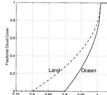
reaches unity.FCis assumed to be zero when RH is less than RHmin and unity when RH is greater than RHmax. Figure 2

displays these curves for ocean and land. Smaller values of RHminare associated with greater subgrid variability. Typical

values for RHmin range from 60 to 100% depending on a

variety of factors, including the vertical level [Sundqvist, 1988], the surface characteristics [Sundqvist et al., 1989], and the model resolution. The threshold over land is often specified lower than the threshold over ocean due to sub-grid-scale surface heterogeneities that translate upward into the atmo-sphere [Sundqvist et al., 1989]. These heterogeneities can result from variable topography, soil moisture, vegetation, surface friction, etc. The ocean surface is relatively homogeneous in that the surface roughness is small and temperatures do not vary considerably at small scales.Sundqvist et al. [1989] use 75 and 85% for land and ocean, respectively. Within the boundary layer and at lower temperatures (⬍238 K), they let RHmin

in-crease linearly to a value near unity. Preliminary experiments varying RHminby⫾5% resulted in negligible changes. Thus for

simplicity, we specify RHmin at 80% for land and 90% for

ocean and do not allow RHminto vary in the vertical or with

Figure 1. Plot of the autoconversion threshold (g/kg) versus temperature (K) for SIMEX (solid line) and SUBEX (dashed for land, dotted for ocean).

Figure 2. Plot of the fractional cloud coverage as a function of relative humidity for SUBEX. The dashed curve denotes the values for land and the solid line denotes the values for ocean.

temperature. RHmax is set to 1.01, allowing water vapor

con-tent to exceed the saturation value by 1%.

The formulation for the autoconversion of cloud water into precipitation in SUBEX is nearly identical to that in SIMEX. The main difference is in the specification of the autoconver-sion threshold and that in-cloud values of Qc are used, as

follows:

P⫽Cppt共Qc/FC⫺Qcth兲FC. (4)

As SIMEX, when precipitation is formed, it is assumed to fall instantaneously. The new autoconversion threshold is based on the analysis of Gultepe and Isaac[1997]. They used aircraft observations of cloud liquid water content and related them to temperature. Here the threshold is obtained by scaling the median cloud liquid water content equation according to the following:

Qcth⫽Cacs10⫺0.49⫹0.013T, (5)

where T is temperature in degrees Celsius, and Cacs is the

autoconversion scale factor. By scaling theQc-T relationship,

we assume that the threshold takes the shape of the mean cloud conditions. Over the ocean there are typically fewer cloud condensation nuclei than over land. As a result, the cloud droplets over the ocean are larger and hence less buoy-ant than those over land [Rogers and Yau, 1989]. Larger cloud droplets tend to result in more collision and coalescence. Thus continental clouds tend to be thicker than maritime clouds for the same probability of precipitation [Rogers and Yau, 1989]. Because of these land-ocean contrasts we specifyCacsat 0.65

over land and 0.4 over ocean. These values were selected on the basis of series of preliminary experiments. Figure 1 displays the autoconversion thresholds for SUBEX (dashes for land and dots for ocean). Note that in both SIMEX and SUBEX the different sizes of cloud droplets over ocean and land are ac-counted for within the CCM3 radiation package. It should be mentioned that model displays a considerable sensitivity to the specification of Qcth and Cacs. Furthermore (5) does not

ac-count for the presence of cloud ice. In light of this it may be expected that SUBEX underpredicts precipitation since cloud ice increases the autoconversion efficiency (via an increase the amount of CCN [Rogers and Yau, 1989]). This, in turn, is likely to result in too much cloud water and will probably adversely impact radiation budget under these conditions. Neglecting ice physics within clouds is a shortcoming in SUBEX and should be addressed in future work.

2.3. Raindrop Accretion (SUBEX Only)

Raindrop accretion can be an important process under cer-tain climatic conditions [Rogers and Yau, 1989]. In SIMEX, only the cloud water in excess of the autoconversion threshold is allowed to precipitate out (see (1)). Thus when clouds form,

they often linger at or near the autoconversion threshold (in the absence of other atmospheric processes such as cloud evap-oration). In nature, however, when precipitation initiates (ex-ceeds the autoconversion threshold), rain droplets falling through clouds collect and remove a portion of the cloud droplets. Thus neglecting this process can result in an under-prediction of precipitation and overunder-prediction of clouds, par-ticularly in humid regions. Accounting for it allows the cloud water content to fall below the autoconversion threshold when precipitation occurs. SUBEX includes a simple formulation for the accretion cloud droplets by falling rain droplets according to the following relation based onBeheng[1994]:

Pacc⫽CaccQcPsum, (6)

wherePaccis the amount of accreted cloud water,Caccis the

accretion rate coefficient, andPsumis the accumulated

precip-itation from above falling through the cloud. Accretion only takes place in the cloudy portions of the grid cell. For simplic-ity,Psumis assumed to be distributed uniformly across the grid

cell. In other words, no knowledge of the cloud fraction in which the precipitation formed is used. In some cases, this may tend to overestimate the effects of accretion.

2.4. Raindrop Evaporation (SUBEX Only)

As with raindrop accretion, raindrop evaporation can also be an important process under certain conditions [Rogers and Yau, 1989]. In arid regions, a significant quantity of the pre-cipitation that forms often evaporates before it reaches the surface. Neglecting this process may lead to the simulation of excessive precipitation in arid regions [Small et al., 1999a]. SUBEX employs the simple formulation of Sundqvist et al. [1989], as follows:

Pevap⫽Cevap共1⫺RH兲Psum1/ 2, (7)

where Pevap is the amount of evaporated precipitation, and

Cevapis the rate coefficient. More raindrop evaporation occurs

where the air is dry relative to saturation. As with the formu-lation for accretion, Psum is assumed to be distributed

uni-formly across the grid cell. Only raindrops falling through the cloud-free portion of the grid box are allowed to evaporate. Inclusion of this process may also result in a decrease in the number of numerical grid point storms [Molinari and Dudek, 1986].

3. Design of Numerical Experiments

In this section we provide a description of the numerical experiments performed in this study. Each run is initialized on March 15, for each of the following years: 1986, 1987, 1988, 1989, 1990, and 1993. The runs are integrated for 1 year and 17 days (18 days for the simulations initialized in 1987 due to the

Table 1. List of Parameters Used in SUBEX and Their Associated Values

Parameter Land Ocean Units

Cloud formation threshold RHmin 0.8 0.9

Maximum saturation RHmax 1.01 1.01

Autoconversion rateCppt 5⫻10⫺4 5⫻10⫺4 s⫺1

Autoconversion scale factorCacs 0.65 0.3

Accretion rateCacc 6 6 m3kg⫺1s⫺1

Raindrop evaporation rateCevap 1⫻10⫺5 1⫻10⫺5 (kg m⫺2s⫺1)⫺1/2s⫺1

1988 leap year). The first 17 (or 18) days are ignored for model spin-up considerations. The simulation for each year is per-formed twice, one run using SIMEX to represent the large-scale cloud and precipitation processes and another using SUBEX. The pair of simulations for each year is identical except for the choice of large-scale cloud and precipitation scheme.

The simulations are initialized on March 15 so that snow cover can reasonably be initialized at zero. In addition, this gives soil moisture within BATS time to spin-up before the summer when biosphere-atmosphere interactions are most pronounced. Lastly, the simulations are divided into year-long runs to minimize drift in soil moisture.

The years 1986, 1987, 1988, 1989, 1990, and 1993 are se-lected because observation-based data exist for model evalua-tion from the Naevalua-tional Aeronautics and Space Administraevalua-tion (NASA) Earth Radiation Budget Experiment (ERBE) except for 1989, 1990, and 1993 [Barkstrom, 1984], NASA-Langley Surface Radiation Budget data (NASA-SRB) except for 1993 [Darnell et al., 1996; Gupta et al., 1999], and International Satellite Cloud Climatology Project D2 data (ISCCP-D2) [ Ros-sow and Schiffer[1999]. Details on each of these data sets are provided in section 4. In 1988 and 1993 the United States Midwest experienced severe summertime drought and flood, respectively. These years are also selected to determine how SIMEX and SUBEX compare in their response to extreme forcings.

As mentioned in section 2.1, RegCM requires initial and boundary conditions. An accurate representation of these boundary conditions is often essential for many RCM applica-tions. Here we force each simulation at the lateral boundaries using the National Centers for Environmental Prediction (NCEP) reanalysis data [Kalnay et al., 1996]. The NCEP data have a spatial resolution of 2.5⬚ ⫻2.5⬚, are distributed at 17 pressure levels (8 for humidity), and are available at time intervals of 6 hours. Traditionally, RegCM has been forced by 12-hour European Centre for Medium-Range Weather Fore-casts (ECMWF) original IIIb global nonanalysis data [ Bengts-son et al., 1982;Mayer, 1988;Trenberth and Olson, 1992]. The ECMWF data have occasional model improvements that lead to inconsistencies within the product between years. This may

cause problems in studies investigating interannual variability. In addition, the temporal resolution (twice daily) may not fully resolve the diurnal cycle of many processes such as the Great Plains low-level jet [Higgins et al., 1997]. The consistent model and high temporal resolution of the NCEP reanalysis product should provide significant improvements to the ECMWF non-reanalysis used in many RegCM applications. In addition, we made improvements to the interpolation procedure to better represent the data on the model grid. These improvements include a correction for the Gibbs phenomena that occurs as a result of the spectral to latitude-longitude transformation and results in noise in the surface fields (e.g.,⫾50 m in the topog-raphy over the ocean surface). The correction is applied over ocean surfaces by adjusting the surface heights and surface pressure to sea level. Correction is particularly important when the domain boundaries lie over ocean regions (as is often the case here). The SST is prescribed using data provided by the U.K. Meteorological Office (Rayner et al. [1996], one degree grid). The atmospheric fields are initialized using the NCEP reanalysis data. Similar toPal and Eltahir[2000], soil moisture is initialized using a data set that merges soil moisture data from the Illinois State Water Survey (ISWS) [Hollinger and Isard, 1994],Huang et al., [1996], and a climatology based on the vegetation type. The vegetation is specified using the Global Land Cover Characterization (GLCC) data provided by the U.S. Geological Survey Earth Resources Observation System Data Center [Loveland et al., 1999]. This is a state of the art vegetation data set that is derived from 1-km advanced very high resolution radiometer data. These data should vide for a more accurate representation of land surface pro-cesses than those of the original 13 RegCM/MM4 vegetation data types [Haagenson et al., 1989]. The soil texture class is prescribed according to the vegetation characterization.

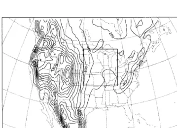
Figure 3 depicts the domain and associated topography for the simulations presented in this study. Close attention has been paid to the selection of the model domain, so the bound-ary conditions do not fully constrain the model. In addition, the number of boundary points occurring over complex topogra-phy have been minimized. The grid is defined on a modified version of the RegCM mercator map projection in that the origin of the projection is no longer constrained to the equator. The added generality minimizes the deviation of the mapscale factors from unity even when compared to the commonly used Lambert conformal map projection. This results in less distor-tion, especially as domain edges are approached. The domain center is located at 37.581⬚N and 95⬚W, and the origin is rotated to 40⬚N and 95⬚W. In the horizontal the grid is 129 points in the east-west direction and 80 in the north-south with a resolution of 55.6 km (approximately half a degree). There are 14 vertical sigma levels with highest concentration of levels near the surface. The model top is at 50 mbar.

4. Model Evaluation Data Sets

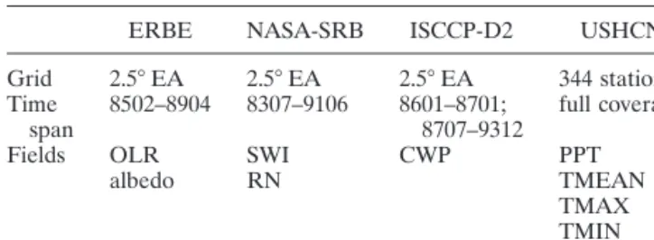
Four data sets are used to evaluate the model performance: ERBE, NASA-SRB, ISCCP-D2, and the U.S. Historical Cli-matology Network (USHCN) data [Karl et al., 1990]. Each of these data sets are completely independent of the NCEP re-analysis data used to force the model. Table 2 provides a summary of the spatial and temporal coverage of the observa-tional fields used to evaluate the model’s performance.

Figure 3. Map of the domain and terrain heights used for the numerical simulations. The outlined box is the region over which spatial averages are taken.

4.1. ERBE Data

The ERBE data are derived from satellite observations of the top of the atmosphere fluxes [Barkstrom, 1984]. They rep-resent the balance between incoming energy from the Sun and outgoing longwave and shortwave energy from the Earth. The data span the period February 1985 through April 1989 and are provided on a 2.5⬚equal-area grid. For convenience, we regrid the data to a 2.5⬚latitude-longitude grid.

In this study we use the top of the atmosphere outgoing longwave radiation and albedo to evaluate the model. Kiehl and Ramanathan [1990] report that the time-averaged accu-racy of the fluxes is within 10 W/m2_{. It is probable, however,}

that the biases vary by region and season. In addition, the uncertainty is likely to be higher when comparing individual months of a particular year.

4.2. ISCCP-D2 Data

The ISCCP-D2 data provide comprehensive cloud property information based on satellite measurements [Rossow et al., 1996; Rossow and Schiffer, 1999]. These data span January 1986 through December 1993 (missing February 1987 through June 1987) and are provided on a 2.5⬚ equal-area grid. For convenience, we regrid the data to a 2.5⬚ latitude-longitude grid. In this study we use the cloud water path measurements to evaluate the model. The D2 product is significantly more accurate than the original C2 product, however, precise num-bers on the accuracy of these data are unclear. To our knowl-edge these are the best measurements of cloud water content available for our purposes.

4.3. NASA-SRB Data

The NASA-SRB is derived from a variety of data sources, including the ISCCP-C1 and ERBE data products [Darnell et al., 1996;Gupta et al., 1999]. To generate the shortwave prod-uct, the ISCCP-C1 and ERBE data are used as input into two different algorithms: the Pinker algorithm [Pinker and Laszlo, 1992] and the Staylor algorithm [Darnell et al., 1992]. The longwave data are generated using the Gupta algorithm [Gupta et al., 1992]. The data span from July 1983 to June 1991, and as the ISCCP-D2 and ERBE data, the NASA-SRB data are pro-vided on a 2.5⬚ equal-area grid. Again, for convenience, we regrid the data to a 2.5⬚latitude-longitude grid.

Gupta et al. [1999] indicate that there are significant biases over coastal regions, snow-/ice-covered regions, regions with high aerosol concentrations, and regions with extensive river and mountain valleys. For model comparison, we use the

in-cident surface shortwave radiation and net surface radiation (net shortwave plus net longwave).Gupta et al. [1999] report a time-averaged bias of 5 W/m2_{and root-mean-square error of}

between 11 and 24 W/m2_{for incident surface shortwave.}

How-ever, when comparing monthly averaged point measurements at individual locations, the biases can be larger than 100 W/m2_.

For our region of interest, we should not expect errors larger than 50 W/m2_{except potentially near the coasts and over the}

Rocky Mountains. In addition,Gupta et al. [1999] suggest that errors ISCCP-C1 input data may pose problems with the NASA-SRB longwave data. This may be problematic for the longwave component of net radiation data used to evaluate the model.

4.4. U.S. Historical Climatology Network Data

The USHCN [Karl et al., 1990] data include monthly aver-aged mean, maximum, and minimum temperature and total monthly precipitation. The data set consists of 1221 high-quality stations from the U.S. Cooperative Observing Network within the 48 contiguous United States and was developed to assist in the detection of regional climate change. The period of record varies for each station but generally includes the period from 1900 to 1996.

The precipitation and temperature data are interpolated onto the RegCM grid defined in section 3. The interpolation is performed by exponentially weighting the station data accord-ing to the distance of the station from the center of the RegCM grid cell, with a length scale of 50 km. In addition, the tem-perature data are corrected for elevation differences between the model and the USHCN data.

5. Results

In this section the simulations utilizing SIMEX to represent the large-scale cloud and precipitation physics are compared to those utilizing SUBEX. Monthly averages from the data are computed over the Upper Midwest defined in Figure 3 and then compared to observations. We focus on the Midwest because it is one of the most agriculturally productive regions in the world. In addition, it is a region that is vulnerable to extreme summer flood and drought. As a result, it is particu-larly important to accurately simulate the energy and water budgets of this region. Furthermore, the observational data used to evaluate the model performance are less likely to have errors due to the relatively flat and homogeneous land surface (see section 4).

Table 3 provides a summary of the statistics computed over the Midwest. The bias between the model simulations and the observational data represents the model’s ability to reproduce observed mean conditions. The root-mean-square error (rmse) provides an indication of the overall error of the model simu-lations compared to the observational data. It should be noted that the rmse contains the bias within the statistic. Therefore an improvement to the bias typically results in an improvement to the rmse. The slope and rmse provide a measure of the model’s ability to simulate the seasonal and interannual vari-ability. A slope greater than unity indicates that the model overpredicts the seasonal and/or interannual variability and a slope less than unity indicates an underprediction. The scatter of the model output around their best fit line to observations describes the accuracy of the model in simulating the processes that represent the interannual variability. Combined improve-ments to the bias, rmse, and slope imply improveimprove-ments to the

Table 2. List of Verification Data Sets Used in This Study

ERBE NASA-SRB ISCCP-D2 USHCN

Grid 2.5⬚EA 2.5⬚EA 2.5⬚EA 344 stations Time

span 8502–8904 8307–9106 8601–8701;8707–9312 full coverage

Fields OLR SWI CWP PPT

albedo RN TMEAN

TMAX TMIN EA denotes equal-area; OLR denotes top of the atmosphere out-going longwave radiation; albedo denotes top of the atmosphere al-bedo; SWI denotes incident surface shortwave radiation; RN denotes net surface radiation; CWP denotes cloud water path; PPT denotes precipitation; and TMEAN, TMAX, and TMIN denote the mean, maximum, and minimum surface temperatures.

model’s ability to accurately represent observations of both the mean conditions and the variability at daily to interannual scales.

5.1. Radiation Budget

In many modeling applications it is crucial to accurately simulate the surface energy budget. To do so, however, it is essential that the atmospheric components of the water and energy budgets are adequately predicted. In this section we evaluate the model’s performance in simulating the top of the atmosphere albedo and outgoing longwave radiation and the surface incident shortwave radiation and net radiation.

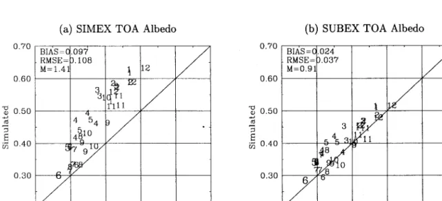
Top of the atmosphere albedo determines the amount of incoming solar radiation that is reflected back into space and can be used as a surrogate for cloud amount. Figure 4 displays the model predictions of top of the atmosphere albedo com-pared to the ERBE observations. In the simulations with RegCM using SIMEX, almost every data point lies above the one-to-one line corresponding to a large bias (0.097), which is nearly equal to the rmse (0.108). This is a clear indication that SIMEX tends to overestimate cloud amount. The slope of the best fit data is 1.41, indicating that SIMEX also overestimates the seasonal variability of albedo and hence cloud coverage.

Most of this overestimation occurs during the warmer months of the year (April through September) where the slope of the data is steeper than 1.41. With this in mind, a correction of the bias alone will not be adequate. Improvements in the seasonal and interannual variability are also required. RegCM using SUBEX to represent the moist physics performs significantly better in reproducing the mean observations of top of the atmosphere albedo (bias⫽0.024). SUBEX also performs con-siderably better in representing the seasonal and interannual variability of albedo (slope ⫽0.91). In addition, there is re-duced scatter about best fit and one-to-one lines of the model data against observations (rmse⫽0.037). Although there are improvements to this scatter, a significant amount still remains. Top of the atmosphere outgoing longwave radiation is also a key component of the atmospheric energy balance and can be used as a measure of cloud height (i.e., cloud top temperature). Figure 5 displays the top of the atmosphere outgoing longwave radiation for both SIMEX and SUBEX against the ERBE observations. RegCM with SIMEX substantially underesti-mates the outgoing longwave radiation, indicating that there are too many high clouds. This is reflected in the low bias of 19.3 W/m2_{, which nearly equals the rmse (22.6 W/m}2_{) and is}

consistent with the SIMEX overestimation of albedo seen above. Also, as is consistent with above, there tends to be an overestimation of the seasonal and interannual variability of clouds (especially during the spring and summer months) re-flected in the large slope of the best fit line (1.42). RegCM, with SUBEX, performs significantly better than SIMEX in simulating the top of the atmosphere outgoing longwave radi-ation. The bias and RMSE are reduced to 0.5 and 8.2 W/m2_,

respectively. Furthermore, both the slope of the best fit line (1.24) and the scatter of the simulation data about the best fit line to observations are considerably reduced, suggesting that SUBEX performs better in representing the seasonal and in-terannual variability. Much of this improvement in the sea-sonal variability is a result of improvements during the spring and summer months, however, an overestimation of the vari-ability still remains during these months. These above im-provements indicate that SUBEX outperforms SIMEX over

Figure 4. Plot of the simulated top of the atmosphere albedo (y axis) against the ERBE observations (x axis). Each data point represents a spatial average over the box outlined in Figure 3. Each digit indicates the month over which the average is taken. The large numbers 5 and 6 refer to May and June of the drought year (1988). (a) SIMEX, (b) SUBEX.

Table 3. Summary of Model Simulation Statistics Compared to Observations for SUBEX and SIMEX Over the Midwest (Outlined in Figure 3)

SIMEX SUBEX

Bias rmse Slope Bias rmse Slope Albedo 0.097 0.108 1.41 0.024 0.037 0.91 OLR ⫺19.3 22.6 1.42 0.5 8.2 1.24 SWI ⫺26.2 30.9 1.03 ⫺3.9 13.2 1.01 RN ⫺20.3 22.9 0.96 ⫺9.9 13.4 1.03 CWP 64.6 74.3 1.22 ⫺17.3 31.2 0.14 PPT ⫺0.37 0.72 0.62 ⫺0.06 0.65 0.73 TMEAN ⫺1.10 2.00 0.98 ⫺0.25 1.15 1.00 TMAX ⫺2.12 2.96 1.05 ⫺0.81 1.65 1.04 TMIN 1.24 1.99 0.92 1.68 1.98 0.97

the Midwestern United States in reproducing the atmospheric radiation budget, as well as the vertical distribution of clouds. Incident surface shortwave radiation is the main energy in-put to the hydrologic cycle of the surface. It reflects the inte-grated effect of the clouds that lie above the biosphere. Figure 6 shows that the improvements in the prediction of the atmo-spheric radiation budget (top of the atmosphere albedo and outgoing longwave radiation) also translate into improvements in the prediction of incident surface shortwave radiation. In the SIMEX simulations the model tends to underestimate incident shortwave radiation at the surface over the Midwest region in nearly every month. This is reflected in the overall low bias of 26 W/m2 _{and the rmse of 31 W/m}2_{. These results are also}

consistent with the SIMEX overprediction of top of the atmo-sphere albedo and underprediction of top of the atmoatmo-sphere outgoing longwave radiation. Although the slope is near unity (1.03), SIMEX tends to overestimate the seasonal variability during months of high incident shortwave radiation (as with the above findings). The simulations using SUBEX do a much better job in reproducing the NASA-SRB data over the Mid-west. The bias and rmse are substantially reduced to⫺4 and 13 W/m2_{, respectively. Furthermore, the slope of the data (1.01) is}

near unity, and the scatter of the data about the best fit line (and one-to-one line) is considerably reduced, indicating that SUBEX is able to better reproduce the seasonal and interan-nual variability of the incoming solar radiation. In addition, the tendency for the model to overestimate the seasonal variability during spring and summer months has been reduced but not completely removed.

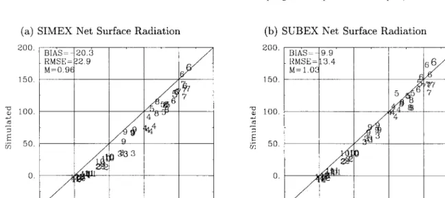
Net surface radiation is a key component of the surface energy budget. It determines the turbulent fluxes into the at-mospheric boundary layer. Figure 7 displays the simulation results against the NASA-SRB data. Consistent with above, SUBEX outperforms SIMEX. The bias is reduced from⫺20 to ⫺10 W/m2 _{and the rmse is reduced from 23 to 13 W/m}2

between SUBEX and SIMEX, respectively. The scatter about the best fit line also improves in the SUBEX simulations. Again, both models tend to overestimate the seasonal variabil-ity during the spring and summer months. This overestimate is somewhat smaller in the SUBEX simulations.

Figure 8 displays the improvement (or deterioration) seen in

the simulated net surface radiation between SUBEX and SIMEX averaged over the entire simulation period. On the whole, improvements (solid contours) result over the entire domain when using SUBEX to represent the large-scale cloud and precipitation processes. Two exceptions lie in coastal re-gions off Southern California and Sinaloa, Mexico. This dete-rioration may be partly explainable by significant biases over coastal regions in the NASA-SRB data (see section 4.3 or Gupta et al. [1999]). The largest improvements are observed over the Pacific Northwest and the Atlantic Ocean. These are both regions where SIMEX tends to overestimate cloud amounts. Over the majority of North America, there is a 6–10 W/m2 _{improvement. There is some seasonal dependence in}

that the improvements tend to be largest in the spring and smallest in the summer (not shown). Lastly, all of the improve-ments resulted from an increase in the simulation of net surface radiation (dark shading).

Overall, RegCM, using SUBEX, results in substantially bet-ter performance in representing the atmospheric and surface energy budgets. The biases in all components of the radiation budget were reduced to values near zero. In addition, the representation of seasonable variability is improved. However, an overestimate (but reduction when compared to SIMEX) in the variability remains during the spring and summer months. This may point to deficiencies in the representation of convec-tive cloud cover and water, since this problem occurs primarily in convectively active months. The following subsection inves-tigates whether the improvements in the energy budget result in improvements to the water budget.

5.2. Water Budget

To demonstrate the water budget, we compare the model to observations of cloud water path and precipitation. Figure 9 compares the model results to the ISCCP-D2 observations of cloud water path for both SIMEX and SUBEX. As alluded to above, SIMEX tends to significantly overestimate cloud water path over the Midwestern United States. The bias is 65 g/m2

and the rmse is 74 g/m2_{. These values are comparable to the}

size of the observed cloud water contents in this region. This overestimate is consistent with the results of the energy budget in that too little shortwave radiation reaches the surface, too

little longwave radiation leaves the top of the atmosphere, and the top of the atmosphere albedo is too high. In addition, SIMEX overestimates the seasonal and interannual variability reflected in the slope (1.22) and scatter of the data about the best fit line. SUBEX performs letter in representing observed mean cloud water path conditions. The bias and rmse have been reduced to⫺17 and 31 g/m2_{, respectively. Although this}

is a significant improvement, SUBEX overcorrects the sea-sonal and interannual variability problem observed in SIMEX (slope ⫽ 0.14). More specifically, it tends not to accurately represent the high cloud amounts observed in November, De-cember, and January. The reason for this may have to do with an artificial cap placed on the cloud water path of 400 g/m2_.

Without this cap, RegCM using SIMEX often overestimates cloud water path by an order of magnitude. SUBEX retains this cap, which may be a large portion of the reason why it underestimates cloud water path in the cloudier months. In addition, the lack of ice phase within SUBEX cloud physics may contribute to the deficiencies.

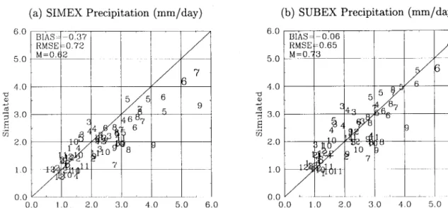
Precipitation is the most important variable of the surface water budget and is probably the most difficult to simulate. Figure 10 shows that improvements in the prediction of the radiation budget result in improvements of the prediction of precipitation over the Midwest. SIMEX underestimates pre-cipitation by 0.37 mm/d and contains significant variability in the error (rmse ⫽ 0.72 mm/d). In addition, it significantly underestimates the seasonal variability (slope⫽0.62). Of par-ticular importance, extreme wet precipitation events (greater than 3 mm/d), which typically occur in the spring and summer in the Midwest, tend to be underrepresented. In the simula-tions using SUBEX, the precipitation bias is significantly re-duced (⫺0.06 mm/d), while the rmse still remains high (0.65 mm/d). In addition, there is a significant improvement in the simulation of the seasonal and interannual variability (slope⫽ 0.73); SUBEX does a considerably better job in representing the high extremes in precipitation. Note that June and July of the flood year (1993, denoted by the large numbers 6 and 7 in the top right-hand portion of the plot) now fall close to the

Figure 6. Plot of simulated incident surface shortwave radiation in W/m2_{(y axis) against the NASA-SRB}

data (x axis). Each data point represents a spatial average over the box outlined in Figure 3. Each digit indicates the month over which the average is taken. The large numbers 5 and 6 refer to May and June of the drought year (1988). (a) SIMEX, (b) SUBEX.

observed values. In addition, both schemes do a particularly poor job in simulating September 1986 and 1993. It is deter-mined that the large-scale and mesoscale dynamics were poorly simulated during these months (too much northerly flow, too little southerly flow (not shown)). Neglecting these months would provide some correction to the low slopes. The mechanisms resulting in the improved simulation of extreme wet precipitation events are described in section 5.4.2.

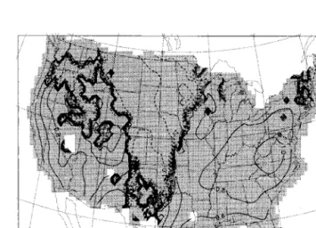
Figure 11 displays the improvement (or deterioration) seen in the simulated precipitation between SUBEX and SIMEX over the United States averaged over the entire simulation

period. (Note that contours only exist over the United States since the USHCN data do not exist elsewhere.) On the whole, improvements (solid contours) result over the majority of the United States when using SUBEX as compared to SIMEX to represent the large-scale cloud and precipitation processes. Exceptions (dashed contours) tend to lie along Pacific and Atlantic coastlines and in the Southwest United States. In SUBEX, east of the⬃103⬚W (Rocky Mountains); most of the improvements result due to an increase in precipitation (dark shading). There tends to be a degradation in performance where the precipitation decreases (light shading). In contrast, to the west⬃103⬚W, most of the improvements occur due to a decrease in precipitation. The performance typically decreases when precipitation increases. In general, SUBEX is able to better represent the processes responsible for precipitation in the different regimes of the United States.

Overall, SUBEX significantly improves the representation of the water budget over the midwestern United States. These improvements, however, are not so large as those seen with the energy budget (see section 5.1). The benefits to the mean conditions of energy budget are primarily due to improvements in the overall cloud amount (see Figure 9). The reason for the improvements to the seasonal and interannual variabilities are more difficult to identify. It is probable that the variable frac-tional cloud coverage (see (3) and Figure 2) plays an important role in these improvements.

5.3. Surface Temperature

As precipitation, surface temperature is also one of the most difficult fields to accurately predict due to its dependence on a variety of factors. This subsection compares the SIMEX and SUBEX simulations to the USHCN observations of mean, minimum, and maximum surface temperature. Note that model temperatures have been adjusted to reconcile differ-ences between station and model elevation.

Figure 12 compares the predictions of mean surface tem-perature from each cloud model to observations. SIMEX tends to significantly underestimate the mean surface temperature

Figure 8. Plot of the overall changes to the net surface radi-ation results between SIMEX and SUBEX averaged over the entire simulation period. Contours display the rmse difference between SIMEX and SUBEX in W/m2_{. Positive values (solid}

lines) indicate that the model simulations improved when us-ing SUBEX, and negative values (dashed lines) indicate a deterioration. The shading displays direction of the difference between SIMEX and SUBEX. Dark shading indicates that SUBEX simulates more net surface radiation than SIMEX and vice versa.

Figure 9. Plot of the simulated cloud water path in g/m2_{(y axis) against the ISCCP-D2 observations (x}

axis). Each data point represents a spatial average over the box outlined in Figure 3. Each digit indicates the month over which the average is taken. The large numbers 5 and 6 refer to May and June of the drought year (1988) and the large numbers 6 and 7 refer to June and July of the flood year (1993). The June 1988 value lies in the bottom left corner. (a) SIMEX, (b) SUBEX.

(bias ⫽ ⫺1.10⬚C) and contains a fair amount of variability (rmse⫽ 2.00⬚C). The overall seasonal variability is well rep-resented (slope⫽0.98), although significant biases occur dur-ing the transition seasons (sprdur-ing and autumn). The best per-formance occurs during the consistent regimes (summer and winter). These two factors imply that simply removing the bias within the parameters of the SIMEX is unlikely to be satisfac-tory. When using SUBEX, the simulation of mean surface temperature significantly improves. The bias and rmse are re-duced to⫺0.25⬚and 1.15⬚C, respectively. Although the slopes

from both sets of simulations are similar (slope ⫽ 1.00 in SUBEX), SUBEX performs better in simulating the seasonal variability of mean surface temperature. A significant portion of the low bias that exists in the SIMEX simulations during the transition seasons is removed. This improvement does not oc-cur at the expense of the summer and winter months. These overall results suggest that RegCM using SUBEX is better able to represent the processes that determine the interannual vari-ability than RegCM using SIMEX.

Figure 13 displays the improvement (or deterioration) seen in the simulated mean surface temperature between SUBEX and SIMEX over the United States averaged over the entire simulation period. Note that contours only exist over the United States since the USHCN data do not exist elsewhere. On the whole, improvements result over the majority of the United States when using SUBEX over SIMEX to represent the large-scale cloud and precipitation processes. However, large degradations in the performance occur over a significant portion of the United States. This region is strikingly corre-lated, areas where the model elevation exceeds the USHCN elevation by more than 200 m. It is plausible that the applied elevation correction is not reasonable when the model terrain and USHCN terrain differ significantly.

Maximum temperature (Figure 14) displays properties sim-ilar to those for mean surface temperature. In SIMEX there is a low bias of 2.12⬚C, a rmse of 2.96⬚C, and a slope of 1.05. The low bias is consistent with the underprediction of incident surface shortwave radiation. As with mean surface tempera-ture, the SIMEX simulations tend toward a cold bias during the transition seasons and have little bias during the consistent regimes. SUBEX is able to correct a significant portion of the biases observed during the spring and autumn months; how-ever, there is still room for improvement. The overall bias, rmse, and slope of the simulation using SUBEX are⫺0.81⬚, 1.65⬚, and 1.04⬚C, respectively. These results suggest improve-ments in the ability of SUBEX to simulate the interannual variability of maximum surface temperature.

Figure 10. Plot of the simulated precipitation in mm/d (yaxis) against the USHCN observations (xaxis). Each data point represents a spatial average over the box outlined in Figure 3. Each digit indicates the month over which the average is taken. The large numbers 5 and 6 refer to May and June of the drought year (1988) and the large numbers 6 and 7 refer to June and July of the flood year (1993). The June 1988 value lies in the bottom left-hand corner in both subplots. (a) SIMEX, (b) SUBEX.

Figure 11. Plot of the overall changes to the precipitation results between SIMEX and SUBEX averaged over the entire simulation period. Contours (United States only) display the rmse difference between SIMEX and SUBEX in mm/d, posi-tive values (solid lines) indicate that the model simulations improved when using SUBEX and negative values (dashed lines) indicate a deterioration. The shading displays direction of the difference between SIMEX and SUBEX. Dark shading indicates that SUBEX simulates more precipitation than SIMEX and vice versa.

The results for minimum surface temperature are presented in Figure 15. The simulations using SIMEX have a significant warm bias of 1.24⬚C and a rmse of 1.99⬚C. In addition, the overall seasonal variability is somewhat underrepresented (slope⫽0.92); most of the underrepresentation occurs during colder months (December through March). SUBEX tends to overestimate minimum surface temperature even more so than SIMEX (bias⫽1.68⬚C). The rmse (1.98⬚C), however, remains nearly the same as with SIMEX. Since the bias is part of the rsme, the variability of the simulation data about the one-to-one line decreases in SUBEX. This suggests that processes representing the variability in minimum surface temperature are better represented in SUBEX. However, the processes that represent the mean conditions are not so well represented as they are in SIMEX. With the decrease in cloud amount seen in Figure 9, one may expect a decrease in the longwave radiation emitted toward the land surface and hence a decrease in night-time (minimum) surface temperatures. Upon further inspec-tion, however, it is evident that the increase in net surface radiation (Figure 7) and associated increase in ground heat flux (not shown) resulted in an increase in minimum surface temperature. This is further reinforced by the increased heat capacity of the soils due to an increase soil moisture (not shown) from the overall increase in precipitation (Figure 10). In addition, the water vapor content of the air in the lower atmosphere tends to be larger in the SUBEX simulations (not shown) resulting in an enhanced greenhouse effect for water vapor also increasing the nighttime temperatures. These fac-tors suggest an inconsistency between the biosphere model (BATS) and the overlying atmospheric processes. It should be expected that if the atmospheric water and energy budgets are improved, the land surface water and energy budgets should also improve. This is not the case with mean conditions (bias) of minimum surface temperature. Lastly, SUBEX performs slightly better in representing the seasonal variability of mini-mum surface temperature (slope⫽0.97).

Despite the increase in the bias in minimum surface tem-perature, RegCM using SUBEX to represent the large-scale

cloud and precipitation processes results in significant im-provements to the simulation of the surface temperature fields.

5.4. Simulation of Extreme Precipitation Events

In the summer of 1988 the U.S. Midwest experienced its warmest and driest summer since the dust-bowl era of the 1930s (Figure 16a) [Ropelewski, 1988]. In contrast, record high rainfall and flooding occurred and persisted throughout much of the summer during 1993 (Figure 16b)Kunkel et al. [1994]. This section investigates how the choice of the large-scale cloud and precipitation scheme impacts the simulation of the above extreme events.

5.4.1. The 1988 drought. Figure 16a displays the USHCN observed precipitation over the United States averaged over May and June 1988, the most extreme drought months. With a few regional exceptions, most of the continental United States received less than 2 mm/d of rainfall during May and June 1988.

Figure 12. Plot of the simulated mean surface temperature in⬚C (yaxis) against the USHCN observations (xaxis). Each data point represents a spatial average over the box outlined in Figure 3. Each digit indicates the month over which the average is taken. The large numbers 5 and 6 refer to May and June of the drought year (1988) and the large numbers 6 and 7 refer to June and July of the flood year (1993). The June 1988 value lies in the top right-hand corner. (a) SIMEX, (b) SUBEX.

Figure 13. Similar to Figure 11 but for mean surface tem-perature in⬚C.

Figure 17 displays the precipitation for both the SIMEX and the SUBEX simulations averaged over the same period (May and June 1988). Both schemes do an excellent job in simulating the observed lack of precipitation over the United States. However, the individual features of the precipitation are not perfectly simulated in either scheme. This may in part be due to the somewhat unpredictable nature of precipitation (espe-cially convective) and also may in part be due to the represen-tation of the boundary conditions and model physics. SIMEX predicts the precipitation distribution over the Gulf Coast states slightly better than SUBEX, while SUBEX better rep-resents the distribution along the eastern seaboard states. The precipitation amounts over the Midwest in May and June 1988 seem to be slightly overpredicted in SUBEX due to increases in both convective and nonconvective precipitation (especially in May). In SUBEX, clouds form earlier than in SIMEX due to the lower relative humidity threshold (0.8 in SUBEX, 1.0 in SIMEX) which increases the likelihood of clouds. In addition, SUBEX has a lower autoconversion threshold (see Figure 1), reducing the average cloud water path (see the large numbers 5 and 6 in Figure 9). Under such conditions, these two effects

result in an increase in nonconvective precipitation (not shown). Furthermore, the increase in incident surface short-wave radiation (see the large numbers 5 and 6, Figure 6) from the decrease in cloud water path outweighs the decrease in net surface longwave radiation resulting from the warmer surface temperatures and lower cloud amount. This tends to result in an increase in net surface radiation (see the large numbers 5 and 6, Figure 7), yielding in an increase in convective precip-itation (not shown). This mechanism appears to be responsible for the increase in May and June 1988 precipitation seen in the SUBEX simulations. Overall, it is difficult to argue that one scheme performs better than the other for the drought of 1988. Most importantly, both models are able to simulate the overall lack of observed precipitation. Furthermore, it should be noted that these results for the 1988 drought are similar to those shown in the Project to Intercompare Regional Climate Sim-ulations in that the general lack of precipitation was captured though the details were simulated less well [Takle et al., 1999].

5.4.2. The 1993 flood. Much of the upper Midwest re-ceived greater than 4 mm of precipitation per day during June and July 1993 (Figure 16b). Peak values above 8 mm/d

oc-Figure 14. Similar to Figure 12 but for maximum surface temperature.

curred over much of Iowa, Nebraska, Missouri, and Kansas. The largest peak (⬃10–11 mm/d) occurred along the Iowa-Missouri border. A smaller peak occurred along the coast of Mississippi and Louisiana (⬃6–7 mm/d).

Figure 18 displays the simulated rainfall for both large-scale cloud and precipitation schemes averaged over June and July 1993. SIMEX is able to simulate the region over the upper Midwest in which rainfall exceeds 4 mm/d. However, it is not able to simulate the precipitation in excess of 8 mm/d which occurred over much of Iowa, Nebraska, Missouri, and Kansas. SUBEX not only simulates the flood region but also simulates the region in excess of 8 mm/d more accurately. The general location of the flood region, however, is simulated too far to the north and east of observed. In addition, the peak maximum is underestimated by⬃2 mm/d. Lastly, both models more or less perform adequately in representing the distribution of precipitation in the rest of the United States. For example, they capture the precipitation peak observed along the coast of Mississippi and Louisiana and the surrounding dry Gulf Coast region. Overall, both models perform well in capturing the spatial distribution of precipitation observed in June and July

1993; however, SUBEX better simulates the magnitude of the flood peak.

The reasons that SUBEX more accurately represents the 1993 summer flooding over the upper Midwest are both di-rectly and indidi-rectly related to the simulation of cloud water path. First, the lower autoconversion threshold specification (see Figure 1) results in an increase in the amount of cloud water that is converted to nonconvective precipitation. Second, the reduction in cloud water results in an increase in incident surface shortwave radiation. This yields an increase in the energy available for convection and results in an increase con-vective precipitation (not shown). Lastly, the increase in soil moisture resulting from the increase in precipitation is also likely to have enhanced the precipitation during the summer of 1993.

6. Summary and Conclusions

A simple, yet physically based, large-scale cloud and precip-itation scheme, which accounts for the subgrid variability of clouds, is presented (SUBEX). Also highlighted are significant modifications made to the specification of the initial and boundary conditions of atmospheric and biospheric variables.

Figure 16. USHCN observations of precipitation in mm/d. Contour interval is specified at 1 (mm/d). Shading occurs at values above 2 mm/d and at intervals of 2 mm/d. Note that the USHCN observations only exist over the United States. (a) The 1988 May and June average, (b) 1993 June and July average.

Figure 17. The 1988 May and June simulated U.S. precipi-tation (mm/d). Contour interval is specified at 1 (mm/d), and shading occurs at values above 2 mm/d and at intervals of 2 mm/d. (a) SIMEX, (b) SUBEX.

Two sets of simulations each consisting of six 1-year runs are performed over North America using RegCM with the moist physics from two different schemes: SIMEX and SUBEX. The only difference between the sets of simulations is the repre-sentation of large-scale cloud and precipitation processes. The sets of the simulations are compared to observations of various radiation and cloud fields from satellite-based data sets and precipitation and surface temperature from surface station-based data sets.

Overall, SUBEX significantly improves the model’s simula-tion of the energy and water budgets. The most significant improvements occur in the prediction of the radiation fields (incident surface shortwave radiation, net surface radiation, outgoing longwave radiation, and albedo) and in the prediction of extreme wet precipitation events (namely, the summer of 1993). Not only does SUBEX reduce the biases between the simulation and the observations (except minimum surface tem-perature) but also significantly improves the simulation of the seasonal and interannual variability.

SUBEX proves to be crucial in the simulation of the flood-ing that occurred in the summer of 1993. Without SUBEX the rainfall over the flood region is simulated as only slightly above normal. On the other hand, few major differences are observed between the schemes in the simulation of the spring/summer

drought of 1988. Both models, however, adequately represent the low amounts of observed precipitation.

Overall, SUBEX provides a more accurate representation of the fields that are important to the energy and water budgets. These improvements are seen in both the mean conditions and the variability at daily to interannual scales. The latter suggests that the new scheme improves the model’s sensitivity, which is critical for both climate change and process studies.

Acknowledgments. We are especially grateful to Sonia Seneviratne of ETH for her valuable insight and assistance in performing some of the preliminary simulations and to Filippo Giorgi of ICTP for his guidance and suggestions. In, addition, we thank Erik Kluzek NCAR for providing the framework necessary to implement the NCEP re-analysis boundary conditions, NOAA-CIRES Climate Diagnostics Center for providing the NCEP reanalysis data, and Daniel Lu¨thi of ETH for aid in implementing the rotated Mercator projection and NetCDF output.

References

Anthes, R. A., E. Y. Hsie, and Y. H. Kuo, Description of the Penn State/NCAR Mesoscale Model Version 4 (MM4),NCAR Tech. Rep., TN-282⫹STR, 66 pp., Natl. Cent. for Atmos. Res., Boulder, Colo., 1987.

Arakawa, A., and W. H. Schubert, Interaction of a cumulus cloud ensemble with the large-scale environment, part I,J. Atmos. Sci.,31, 674–701, 1974.

Barkstrom, B. R., The Earth Radiation Budget Experiment (ERBE), Bull. Am. Meteorol. Soc.,67, 1170–1185, 1984.

Beheng, K. D., A parameterization of warm cloud microphysical con-version processes,Atmos. Res.,33, 193–206, 1994.

Bengtsson, L., M. Kanamitsu, P. Kallberg, and S. Uppala, FGGE 4-dimensional data assimilation at ECMWF, Bull. Am. Meteorol. Soc.,63, 29–43, 1982.

Darnell, W. L., W. F. Staylor, S. K. Gupta, N. A. Ritchey, and A. C. Wilber, Seasonal variation of surface radiation budget derived from ISCCP-C1 data,J. Geophys. Res.,97, 15,741–15,760, 1992. Darnell, W. L., W. F. Staylor, N. A. Ritchey, S. K. Gupta, and A. C.

Wilber, New data set on surface radiation budget,Eos,Trans. AGU, Electron. Suppl., February 27, 1996. (Available as http://www.agu/ org/eos_elec, 95183e.html)

Dickinson, R. E., P. J. Kennedy, A. Henderson-Sellers, and M. Wilson, Biosphere-Atmosphere Transfer Scheme (BATS) version 1E as cou-pled to the NCAR Community Climate Model,NCAR Tech. Rep., TN-275⫹STR, 72 pp., Natl. Cent. for Atmos. Res., Boulder, Colo., 1986.

Dickinson, R. E., R. Errico, F. Giorgi, and G. Bates, A regional climate model for the western United States,Clim. Change,15, 383–422, 1989.

Eltahir, E. A. B., and R. L. Bras, Sensitivity of regional climate to deforestation in the Amazon Basin,Adv. Water Resour.,17, 101–115, 1994.

Giorgi, F., Simulation of regional climate using a limited area model nested in a general circulation model,J. Clim.,3, 941–963, 1990. Giorgi, F., and G. T. Bates, The climatological skill of a regional

climate model over complex terrain,Mon. Weather Rev.,117, 2325– 2347, 1989.

Giorgi, F., and L. O. Mearns, Introduction to special section: Regional climate modeling revisited,J. Geophys. Res.,104, 6335–6352, 1999. Giorgi, F., and C. Shields, Tests of precipitation parameterizations available in latest version of NCAR regional climate model (RegCM) over continental United States, J. Geophys. Res., 104, 6353–6375, 1999.

Giorgi, F., Y. Huang, K. Nishizawa, and C. Fu, A seasonal cycle simulation over eastern Asia and its sensitivity to radiative transfer and surface processes,J. Geophys. Res.,104, 6403–6423, 1999. Grell, G. A., Prognostic evaluation of assumptions used by cumulus

parameterizations,Mon. Weather Rev.,121, 764–787, 1993. Grell, G. A., J. Dudhia, and D. R. Stauffer, Description of the fifth

generation Penn State/NCAR Mesoscale Model (MM5), NCAR Tech. Rep., TN-398⫹STR, 121 pp., Natl. Cent. for Atmos. Res., Boulder, Colo., 1994.