2006, Vol. 49, No. 1, 33-48
A NEW OPTIMAL SEARCH ALGORITHM FOR THE
TRANSPORTATION FLEET MAINTENANCE SCHEDULING PROBLEM
Ming-Jong Yao Jia-Yen Huang
Tunghai University Ling Tung University
(Received April 30, 2004; Revised March 18, 2005)
Abstract In this study, we propose a new solution approach for the Transportation Fleet Maintenance Scheduling Problem (TFMSP). Before presenting our solution approach, we first review Goyal and Gu-nasekaran’s [International Journal of Systems Science, 23 (1992) 655-659] mathematical model and their search procedure for determining the economic maintenance frequency of a transport fleet. To solve the TFMSP, we conduct a full analysis on the mathematical model. By utilizing our theoretical results, we propose an efficient search algorithm that finds the optimal solution for the TFMSP within a very short run time. Based on our experiments using random data, we conclude that the proposed search algorithm out-performs Goyal and Gunasekaran’s search procedure.
Keywords: Scheduling, maintenance, mathematical model, algorithm
1. Introduction
In this study, we devote our efforts toward investigating a mathematical model for determin-ing the economic maintenance frequency of a transportation fleet. We name this problem the “Transportation Fleet Maintenance Scheduling Problem”, which is abbreviated as the TFMSP. The mathematical model for the TFMSP was previously proposed by Goyal and Gunasekaran [3]. We extend their work in two aspects: first, we conduct a full theoretical analysis on the theoretical properties of the mathematical model, and second, we propose an efficient search algorithm that solves for the optimal solution in Goyal and Gunasekaran’s [3] model.
As mentioned in [3], the problem of determining the economic maintenance of a machine has been dealt with extensively in management science, operations research, and industrial engineering (see [2], [4], [6], [7], and [8]). But researchers pay limited attention to the problem of determining the operating and maintenance schedules for a transportation fleet. For the rest of this section, we review Goyal and Gunasekaran’s [3] mathematical model for the Transportation Fleet Maintenance Scheduling Problem (TFMSP).
Before presenting the mathematical model, we first introduce the assumptions made and the notation used later. There aremgroups of vehicles, and the number of vehicles in group iis denoted asni.In the TFMSP, the decision maker plans the maintenance schedules of the vehicle groups in some basic period, denoted byT, (e.g., in days, weeks, or bi-weeks, etc.). The maintenance work on a group of vehicles is carried out at a fixed, equal-time interval that is called themaintenance cycle for that group of vehicles. The vehicles in the ithgroup
are sent for maintenance once inki basic periods where ki is a positive integer. (Therefore, the maintenance cycle for the vehicles in the ith group iskiT.) We note that the model for the TFMSP is for planned maintenance, and the model does not consider unplanned fleet
vehicle failure in the scheduling of fleets.
We consider two categories of costs in the TFMSP, namely, the operating cost and the maintenance cost. The operating cost of a vehicle depends on the length of the maintenance cycle, and it is assumed to increase linearly with respect to time since the last maintenance on the vehicle. Specifically, the operating cost per unit of time at time t after the last maintenance for a vehicle in group i is given by fi(t) = ai +bit where ai is the fixed cost and bi indicates the increase in the operating cost per unit of time. For each vehicle in group i, we also assume that it takes Xi units of time for its maintenance work. And the utilization factor of a vehicle in the ith group on the road is Y
i , where Xi and Yi are
known constants. (One may refer to [10] for further discussions on the utilization factor of a vehicle.) Therefore, the actual time during which a vehicle can operate is equal to Yi(kiT −Xi), and the total operating cost for a vehicle in groupi is given by
Yi(kiT−Xi) 0 fi(t)dt = Yi(kiT−Xi) 0 (ai+bit)dt = Yi(ai−biXiYi)kiT + 0.5biYI2k2iT2−XiYi(ai−0.5biXiYi) (1.1) The fixed cost of starting the maintenance for a vehicle in group i is given by si. On the other hand, as maintenance work is carried out at intervals of T, a fixed cost, denoted by S, will be incurred for all vehicle groups scheduled for maintenance in each basic period.
The objective function of the TFMSP is to minimize the average total costs occurred per unit of time. Therefore, we divide the cost terms of each vehicle by its cycle time respectively to obtain their corresponding terms in the objective function. By the derivation above, the mathematical model for the TFMSP can be expressed as problem (P0).
(P0) minZ((k1, k2, . . . , km), T) = S T + m i=1 Φi(ki, T) +u (1.2) where Φi(ki, T) = niC1i kiT +niC2ikiT, C1i =si−XiYi(ai−0.5biXiYi) andC2i = 0.5biYi2. Also, u=m i=1
niYi(ai−biXiYi) is a constant since all the parameters are given in its expression. Then, solving the problem (P0) is equivalent to obtaining the optimal solution for the problem (P) as follows. (P) Ψ(k1, k2, . . . , km), T) = inf T >0{ S T + m i=1 Φi(ki, T)|ki ∈N+, i= 1, . . . , m)}. (1.3) In the TFMSP, the decision maker needs to determine T (i.e., the basic period) and (k1, k2, ..., km) (i.e., the frequency of maintenance for vehicles in each group) so as to mini-mize the total costs incurred per unit of time.
We outline the organization of this paper as follows: We will review the studies in the literature for the Transportation Fleet Maintenance Scheduling Problem in the second section. Then, in Section 3, we present a full theoretical analysis on the optimal cost curve of the problem (P).Based on our theoretical results, we derive an effective search algorithm that efficiently solves the TFMSP in Section 4. In the first part of Section 5, we employ a numerical example to demonstrate the implementation of the proposed algorithm. Then, we use randomly generated examples to show that the proposed algorithm significantly outperforms Goyal and Gunasekaran’s search procedure in the second part of Section 5. Finally, we address our concluding remarks in Section 6.
2. Literature Review
In this section, we review the studies in the literature for the Transportation Fleet Mainte-nance Scheduling Problem.
We first review the solution approach proposed in Goyal and Gunasekaran’s [3] paper. The algorithm is based on two equations that are derived by setting the first derivative of Z((k1, k2, . . . , km), T) with respect to the decision variables to zero:
T(k1, k2, . . . , km) = S+m i=1 niC1i ki m i=1 niC2iki (2.1) ki∗(T) = C1i C2i 1 T (2.2)
Goyal & Gunasekaran’s search procedure
1. For the first iteration, assume ki = k(0)i = 1 for all i, and obtain the first estimate of T =T(1) from (2.1). At T =T(1), determine ki =ki(1) from (2.2) for all i. Ifki(1) values are not integers, then select the nearest non-zero integer.
2. Using ki = ki(1) from (2.2) for i = 1, . . . , m, obtain T = T(2) from (2.1) and then ki =k(2)i from (2.2) using T =T(2). Repeat the process until the rth iteration and stop
when k(ir) =ki(r−1) for i = 1, . . . , m. The economic policy is obtained at T∗ =T(r) and
ki∗ =k(ir).
Later, van Egmond, Dekker & Wildeman [9] discussed Goyal and Gunasekaran’s search procedure. They indicated that the function Z((k1, k2, . . . , km), T) is not convex as Goyal and Gunasekaran assumed in [3]. Since the values ofki need to be integers, the determination of the global optimization is not as easy as Goyal and Gunasekaran suggested. They also showed that it is not necessarily the ki minimizing Z when one rounds (2.2) to the nearest non-zero integer. Finally, they indicated that Goyal and Gunasekaran’s search procedure often stops after its first iteration without obtaining an optimal solution. These three problems explain why Goyal and Gunasekaran’s solution does not always obtain an optimal solution. In fact, it is often stuck in a local optimal solution.
However, van Egmond, Dekker & Wildeman [9] only mentioned that one needs to try different starting values to find an optimal solution, but without proposing a new solution approach to solve the TFMSP.
To the best of the authors’ knowledge, there exists no solution approach that can find an optimal solution for the TFMSP. Therefore, we are motivated to propose a new solution approach towards this aim in this study.
3. Theoretical Analysis
In this section, we discuss some theoretical analyses that provide insights into the optimal cost function of Ψ((k1, k2, . . . , km), T).Our theoretical analyses facilitate the derivation of the search algorithm presented in Section 3.
By observing the right-side of (1.3), we learn that the terms are separable. Therefore, we are motivated to study the properties of Φi(ki, T) since they will establish the foundation for further investigation of the function Ψ((k1, k2, . . . , km), T).
Proposition 3.1. For any given ki ∈ N+, the function Φi(ki, T) satisfies the following properties for T >0, i∈ {1, . . . , m}.
1. Φi(ki, T) is strictly convex;
2. Φi(ki, T) has a minimum for T =x∗i/ki with x∗i given by
x∗i =C1i/C2i (3.1)
3. The function Φi(ki, T) obtains its minimal objective function value by
2niC1iC2i (3.2)
Proof. We may prove these assertions using simple algebra.
Let us define a new function gi(T) by taking the optimal value of ki at any value T >0 for the function Φi(ki, T) as follows.
gi(T) := inf
ki∈N+{
Φi(ki, T)|T =T ∈R+} (3.3) Consequently, the problem (P) can be re-written as
(P1) Γ(T) = inf T >0{ S T + m i=1 gi(T)} (3.4)
where the function Γ(T) is the optimal objective function value of problem (P1) with respect to T.
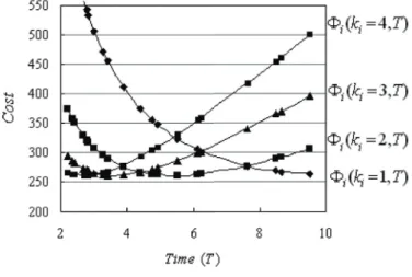
Before further analyzing problem (P1), we first graphically display the curves of the Φi(ki, T) function withki = (1,2,3,4) in Figure 1. Note that the curve of the gi(T) function is actually the lower envelope of the Φi(ki, T) functions.
Figure 1: The curves of the Φi(ki, T) function withki = (1,2,3,4) Importantly, Figure 1 shows two interesting observations on the gi(T) function:
1. The function gi(T) is piece-wise convex with respect to T.
2. Suppose that k∗(w−) and k∗(w+), respectively, are the optimal multipliers of the left-side and right-left-side convex curves with regard to a junction point w in the plot of the gi(T) function. Then,k∗(w−) = k∗(w+) + 1,wherew− =w−ε, w+ =w+εandε→0+. In the following discussion, we will have further analysis on these two observations and will formally prove them as the basis for deriving the theoretical properties for problem (P1).
3.1. The junction point
Next, we define a “junction point” forgi(T) as a particular value ofT where two consecutive convex curves Φi(ki, T) and Φi(ki + 1, T) concatenate. These junction points determine at “what value ofT” where one should change the value ofki so as to obtain the optimal value for the gi(T) function.
We first derive a closed-form for the location of the junction points. We define the difference function ∆i(k, T) by ∆i(k, T) = Φi(ki+ 1, T)−Φi(ki, T) (3.5) = niC1i (k+ 1)T +niC2i(k+ 1)T − niC1i kT −niC2ikT = − niC1i k(K+ 1)T +niC2iT
We note that w is the point where two neighboring convex curves Φi(ki + 1, T) and Φi(ki, T) meet. Importantly, such a junction point w provides us with the information on at “what value of T” where one should change the value of k so as to secure the optimal value for thegi(T) function.
By the rationale discussed above, we derive a closed form to locate the junction points by letting ∆i(k, T) = 0 as follows.
δi(k) = C1i
C2i(k+ 1)k =
2(si−XiYi(ai−0.5biXiYi)
biYi2(k+ 1)k (3.6)
Note that δi(k) indicates the location of the kth junction point of the function g i(T)
(from its right-side). By (3.6), the following inequality (3.7) holds
δi(v)< ... < δi(k+ 1)< δi(k)< ... < δi(2) < δi(1) (3.7) where v is an (unknown) upper bound on the value of k.
Theorem 3.1 is an immediate result from (3.6) and (3.7).
Theorem 3.1. Suppose that k∗(w−) and k∗(w+) are the optimal multipliers of the left-side and right-side convex curves with regard to a junction point w of the gi(T) function, then k∗(w−) = k∗(w+) + 1.
The following corollary is also a by-product of (3.6) and (3.7), and it provides an easier way to obtain the optimal multiplier: ki∗(T)∈N+ for thegi(T) function for any givenT > 0 .
Corollary 3.1. For any givenT >0, an optimal value of k∗i(T)∈N+ for thegi(T)function is given by ki∗(T) = −1 2+ 1 2 1 + 4C1i C2iT2 (3.8) with · denoting the upper-entier function.
Proof. For any given T > 0, an optimal value of k ∈ N+ for the gi(T) function is such that δi(k) ≤ T < δi(k−1). Equivalently, the value of k must satisfy
C1i C2i(k+1)k ≤ T and T < C1i C2i(k−1)k. Therefore, we have k2 +k − C1i C2iT2 0 and k2 −k − C1i C2iT2 < 0. Since k
must be positive, we have −12 + 12
1 + 4C1i C2iT2 ≤ k < 1 2 + 12 1 + 4C1i C2iT2. Thus, we complete the proof.
3.2. Some insights into the optimal cost function
Utilizing our theoretical analyses on the Φi(ki, T) and gi(T) functions one can gain more insight into the Γ(T) function.
First, Propositions 3.2 and 3.3 characterize the Γ(T) function as follows.
Proposition 3.2. The Γ (T) function is piece-wise convex with respect to T.
Proposition 3.3. All the junction points for each group i, will be inherited by the Γ (T) function. In other words, if w is a junction point for a group i, w must also show as a junction point on the piece-wise convex curve of the Γ (T) function.
To make our notation simpler, we define k = (k1, . . . , km) to represent a set of main-tenance frequency. Theorem 3.2 is an immediate result of Theorem 3.1 and Proposition 3.3.
Theorem 3.2. Suppose that k(w−) and k(w+), respectively, are the set of optimal multi-pliers for the left-side and right-side convex curves with regard to a junction point w in the plot of the Γ (T) function. Then, k(w−) is secured from k(w+) by changing at least one of ki byki∗(w−) and ki∗(w+).
4. The Proposed Search Algorithm
In this section, we propose a search algorithm that solves the optimal solution for the problem (P1) in (3.4).
Our theoretical analyses in Section 3 encourage us to solve the problem (P1) by searching along the T-axis. To design such a search algorithm, we first need to define the search range by a lower and an upper bound on the T-axis, which are denoted by Tmin and Tmax, respectively. We note that the bounds Tmin and Tmax are derived by asserting that the optimal solution in [Tmin, Tmax] must be no worse than any solution outside of [Tmin, Tmax]. Also, we must utilize our theoretical analyses on the optimality structure, especially, the properties of the junction points on the Γ (T) function.
In the following discussions, we first discuss how to find initial lower and upper bounds of the search range and how to use an iterative procedure to improve the initial lower and upper bounds. Also, we demonstrate how to use the junction points to proceed with the search. Then, we propose an approach to further improve the lower bound on the search range. Finally, we summarize our proposed search algorithm.
4.1. The initial lower and upper bounds of the search range
First, we present an upper bound on the search range by the Common Cycle (CC) approach in which it requires that ki = 1 for all i, i.e., all the vehicle groups share a common maintenance cycle. We set
TCC = S+ i niC1i / i niC2i (4.1)
where TCC is the optimal maintenance cycle for the CC approach. Next, we will show that it is appropriate to set Tmax=TCC in the following lemma.
Lemma 4.1. For the Γ (T) function, there exist no local minima for T > Tcc.
Denote the optimal objective function value of (P1) and the optimal value of the basic period by Ψ∗and T∗. Next, we derive an initial lower bound on the search range in the following lemma.
Lemma 4.2. The value
β1 = 2S
ΨU (4.2)
serves as a lower bound forT∗ whereΨU is an upper bound on the optimal objective function
value of the problem (P1).
Proof. For any given set of k,its local minimum ˘T(k) is given by ˘T (k)
= S+m i=1 niC1i ki /m i=1
niC2iki.Substituting ˘T (k) into the objective function of the prob-lem (P) in (1.3), one shall obtain its optimal objective function value by
Ψ (k, T) = 2 S+ m i=1 niC1i ki m i=1 niC2iki . (4.3)
By the expressions of ˘T (k) and (4.3), it follows that Ψ∗T∗ >2S, soT∗ >2S/Ψ∗.Given ΨU
is an upper bound on the optimal objective function value of the problem (P1), it obviously holds that T∗ >2S/Ψ∗ since ΨU ≥Ψ∗.
Note that we need an upper bound ΨU to obtain β
1 as indicated in eq. (4.2). The
lower the value of ΨU, the tighter the lower bound β
1. Here, we have an easy way to
obtain a good value of ΨU. First, we shall locate T
0 = mini
0.5C1i/C2i. Denote k∗(T)≡ (k1∗(T), k2∗(T), . . . , km∗(T)) as the set of optimal maintenance frequencies with respect to a given value of T. Then, we obtain the optimal k∗(T0) corresponding to T0 by (3.8). Since the objective function value of any feasible solution serves as an upper bound on Ψ∗, we have an upper bound by ΨU = Ψ(k∗(T0), T0) from eq. (4.3). Consequently, an initial lower bound is obtained byTmin = 2S/ΨU.
Intuitively, if we may shorten the search range on the T-axis, we may reduce the compu-tational efforts in the proposed search algorithm. Therefore, we are motivated to improve the initial lower and upper bounds.
Based on our numerical experiments in our study, we have an interesting observation on the Γ (T) function: the Γ (T) function is monotonically decreasing from Tmin to a value TA, and monotonically increasing from a value TB toTmax. Therefore, if we may determine the values of TA and TB, then we could efficiently confine our search range to [TA, TB]. Before presenting our iterative procedures to determine the values of TA and TB, we discuss their theoretical foundations, i.e., Lemma 4.3, Theorem 4.1 and Corollary 4.1, as follows.
Lemma 4.3. Let ka be the set of optimal maintenance frequencies that minimizes Ψ (·, T)
in the range [Ta
l , Tua]. Let the optimal value of T corresponding to ka be Ta∗. If Tla > Tua,
then the function is monotonically decreasing in [Ta l , Tua].
Next, Theorem 4.1 and Corollary 4.1 lay important foundations for our iterative proce-dures to improve the bounds of the search range.
Theorem 4.1. Letka be the set of optimal maintenance frequencies that minimizesΨ (·, T)
in the range [Ta
l , Tua]. Let the optimal value of T corresponding to ka be Ta∗. If Ta∗ > Tua,
then the Γ (T) function is monotonically decreasing in [Ta l , Ta∗].
Proof. From Lemma 4.3, it is clear that when Ta∗ ≥Tua,the function Ψ(ka, T), which is the same as the Γ (T) function, is monotonically decreasing in [Ta
l, Ta∗]. Now, consider those
sub-intervals of T between Ta
u and Ta∗. Within each of them the optimal set of optimal
maintenance frequencies remains unchanged. Let kb be the set of optimal maintenance frequencies in Tb l, Tub , where Tb l, Tub ⊆ [Ta l, Ta∗], i.e., Tua ≤ Tlb < Tub ≤ Ta∗, We assert
that there exists at least one group i such that kb
i < kia from (3.8) because of Tua ≤ Tlb.
Let the optimal value of T corresponding to kb be Tb∗. As kidecreases, the numerator of ˘ T (k) = S+m i=1 niC1i ki /m i=1
niC2iki increases and the denominator decreases. Therefore, we haveTb
u < Ta∗ ≤Tb∗.Therefore, the Γ (T) function is monotonically decreasing in
Tb l, Tub
by Lemma 4.3. We can repeat the same argument for all the convex sub-intervals of T in [Ta
u, Ta∗].Therefore, the Γ (T) function is monotonically decreasing in [Tla, Ta∗].
Corollary 4.1. Letkabe the set of optimal maintenance frequencies that minimizesΨ(·, T) in the range [Ta
l , Tua]. Let the optimal value of T corresponding to ka be Ta∗. If Ta∗ ≤ Tla,
then the Γ (T) function is monotonically increasing in [Ta∗, Ta u].
Proof. The proof is similar to that of Theorem 4.1.
The basic idea of our iterative improving procedures is summarized as follows. Let ˘
T1(k1) > Tmin be the local minimum for the set of optimal maintenance frequencies
k1. By Theorem 4.1, we assert that the Γ (T) function is monotonically decreasing in
Tmin,T˘1(k1)
. Therefore, one may alternatively find the local minimum ˘T (k) and the set of optimal maintenance frequencieskiteratively to reach the first local minimum to the right of Tmin, i.e., the value of TA mentioned above. In a similar fashion, the first local minimum to the left ofTmax,i.e.,TB , can be determined. Once the improved bounds ofTA and TB are determined, we use the procedure presented in the next section to proceed with the search within the search range.
4.2. Proceed with the search by the junction points
How can one proceed with the search from our initial point TCC to lower values of T? We do this by obtaining k∗(TCC) by (3.8) in Corollary 3.1 where k∗(T) denotes as the set of optimal multipliers at givenT.Then, by Propositions 3.2 and 3.3, each junction pointδi(ki) provides the information whereby one should change the optimal multiplier of groupi from ki to ki+ 1 at δi(ki) to obtain the optimal value for the Γ (T) function. Therefore, during the search, we need to keep an m-dimensional array (δ1(k1), δ2(k2), . . . , δm(km)) in which each value of δi(ki) indicates the location of the next junction point of group i where the optimal multiplier of group ishould be changed. Since the algorithm searches toward lower values ofT,one should change the multiplier for the particular groupiwith the largest value ofδi(ki) to correctly update the set of optimal multipliers. Let Tc be the current value of T where the search algorithm reaches. Denote π as the group index for the group i with the largest value of δi(ki),i.e.,
π = arg max
To proceed with the search from Tc,we need to update the set of optimal multipliers at δi(ki) by
k∗(δπ(kπ))≡(k∗(Tc)\ {kπ})∪ {kπ+ 1} (4.5) where “\” denotes set subtraction.
Note that Theorem 3.2 implies that the set of optimal multipliers k∗ is invariant in each convex sub-interval (i.e., between a pair of consecutive junction points) on the Γ (T) function. Hence, this step actually obtains the set of optimal multipliers for all the values of T ∈ (δπ(kπ), Tc). Then, we should check if the local minimum for k∗(Tc) exists in the convex sub-interval (δπ(kπ), Tc), since such a local minimum could be a candidate for the optimal solution. For any given set of k, one may obtain its local minimum, ˘T (k), by first taking the derivative of the Γ (T) function with respect to T and then, equating it to zero. Therefore, ˘T (k) is given by eq. (4.6) as follows.
˘ T (k) = S+ m i=1 niC1i ki / m i=1 niC2iki (4.6)
4.3. Further improvement on the lower bound
On the other hand, we derive another lower boundβ2 in Lemma 4.4, which is usually tighter than van Ejis’ lower boundβ1.We note that our lower bound β2 is derived by asserting that there exists no solution that obtains a lower objective value than Z
k ˘ T ,T˘ forT < β2.
Lemma 4.4. At a local minimumT ,˘ one may secure a lower bound β2 on the search range by β2 = S S/T˘+m i=1 φi ki∗ ˘ T ,T˘ (4.7) whereφi ki∗ ˘ T ,T˘ = ⎧ ⎨ ⎩ niC1i ˘ T +niC2i ˘ T −2ni√C1iC2i, ki∗ ˘ T = 1 2ni√C1iC2i(ki+ 1)/ki+ki/(ki+ 1) −1 , ki∗ ˘ T >1 ⎫ ⎬ ⎭. Proof. We note that the function φi
k∗i ˘ T ,T˘
indicates the maximum magnitude of decrement in Φ (ki, T) from ˘T to any value of T < T˘ for group i. Recall that Proposition 3.1 asserts that the function Φ (ki, T) is bounded from below by 2ni√C1iC2i. If the optimal multiplier for groupiisk∗i
˘ T
= 1,then the maximum magnitude of decrement ingi(ki, T) from ˘T to any value ofT <T˘ is bounded byniC1i/T˘+niC2iT˘−2n√C1iC2i.Ifki∗
˘ T >1, then gi(ki,T˘)≤max Φi k∗i( ˘T)−1, δi(ki∗( ˘T)−1) ,Φi ki∗( ˘T), δi(k∗i( ˘T)) (4.8) by the piece-wise convexity of the Φi(k∗i( ˘T),T˘) function.
Since one can easily prove that Φi
ki∗( ˘T), δi(ki∗( ˘T)) < Φi ki∗( ˘T)−1, δi(ki∗( ˘T)−1) , it leads to the fact Φi
k∗i( ˘T),T˘ ≤ Φi ki∗( ˘T), δi(k∗i( ˘T)) . By plugging ki∗( ˘T) and δi(ki∗( ˘T)) into the function Φi(ki, T),we have the following concise expression for Φi
ki∗( ˘T), δi(k∗i( ˘T))
after some simplification. Φi
ki∗( ˘T), δi(k∗i( ˘T))
In other words, if ki∗( ˘T)>1, the maximum magnitude of decrement in gi(ki, T) from ˘T to any value of T <T˘ is bounded by 2ni√C1iC2i
((ki+ 1)/ki+ki/(ki + 1))−1 . On the other hand, the major setup cost would increase from S/T˘ to S/T from ˘T to any value ofT < T .˘
The lower bound is derived by asserting that for T ≤ β2, the increment in the major setup cost, i.e., S/T − S/T ,˘ must exceed the maximum magnitude of decrement, i.e.,
m i=1 φi k∗i ˘ T ,T˘ ; or,S/T −S/T˘≥ m i=1 φi k∗i ˘ T ,T˘
,which gives exactly eq. (4.7). The revision of Tmin at the newly-obtained, best-on-hand, local minimum can be sum-marized as follows. Denote K∗ and T∗ as the set of optimal maintenance frequencies and the optimal value of the basic period obtained by the proposed search algorithm. After securing a new local minimum ˘T ,if Ψ(k∗( ˘T),T˘)<Ψ(K∗, T∗), then one should try to revise Tmin = max{Tmin, β1, β2}, where β1 is secured by plugging ΨU = Ψ(k∗( ˘T),T˘) in eq. (4.3) and β2 is obtained from eq. (4.7), respectively.
4.4. The algorithm
We are now ready to enunciate the proposed search algorithm.
1. Obtain the initial lower and upper bounds of the search range using the following steps: (a) Find an initial upper bound: Calculate Tmax=TCC by (4.1).
(b) Find an initial lower bound: Compute T0 = mini0.5C1i/C2i , obtain the optimal
k∗(T0) corresponding to T0 by (3.8). Also, we calculate ΨU = Ψ(k∗(T
0), T0) by eq.
(4.3). Then, obtain an initial lower bound by Tmin = 2S/ΨU.
(c) Let K∗ =k∗(Tmin), T∗ =Tmin and Ψ∗ = ΨU.
2. Improve the bounds of the search range by the following iterative procedures:
(a) Improve the upper bound: Set T0 =Tmax and Told = Tmax. Calculate k∗(T0) corre-sponding to T0 by (3.8). Compute ˘T(k∗(T0)) by eq. (4.6). Set Tmax =T0 (Repeat the above steps until Told/Tmin = 1.)
(b) Improve the lower bound: Set T0 = Tmin and Told = Tmin Calculate k∗(T0) corre-sponding to T0 by (3.8). Compute ˘T(k∗(T0)) by eq. (4.6). Set Tmin =T0 (Repeat the above steps until Tmin/Told = 1.)
3. SetTc =Tmax. If Tc ≤Tmin, then go to step 5. 4. Proceed to the next convex sub-interval:
(a) Set π = arg maxi{δi(ki) < Tc}, k∗(δπ(kπ)) ≡ (k∗(Tc)\{kπ})∪ {kπ + 1}. Then, let Tc =δπ(kπ).
(b) Calculate ˘T(k∗(Tc)) by (4.6) and compute Ψ(k∗(Tc),T˘(k∗(Tc))).
(c) If Ψ∗ ≥Ψ(k∗(Tc),T˘(k∗(Tc))), set Ψ∗ = Ψ(k∗(Tc),T˘(k∗(Tc))),K∗ =k∗(Tc), T∗ =Tc. Also, try to revise the lower bound Tmin byβ2 in eq. (4.7).
(d) Go to Step 3.
5. The optimal solution is given by (K∗, T∗) with the corresponding minimal cost Ψ∗. In many real-world applications, the basic period must take a discrete value; for instance, a day or a week. Still, we could apply the proposed algorithm for those cases after some modifications. First, we should locate the lower bound Tmin and the upper bound Tmax using the first two steps in the proposed algorithm. Next, instead of using Steps 3 and 4 in the proposed algorithm, for each discrete value of T in the interval [Tmin, Tmax], we obtain the corresponding vector of optimal maintenance frequenciesk(T) and its optimal objective function value, i.e., Ψ(k(T), T). Then, we could find an optimal solution by picking the
one with the minimum objective function value. Note that since the objective function value may significantly change after taking the discrete values of T∗orT∗+ 1 from the proposed algorithm directly, we suggest examining the optimal objective function value for each discrete value of T (in the interval [Tmin, Tmax] ).
5. Numerical Experiments
In the first part of this section, we employ a numerical example to demonstrate the imple-mentation of the proposed search algorithm. Then, we use randomly generated instances to show that the proposed search algorithm outperforms Goyal and Gunasekaran’s [3] search procedure.
5.1. A demonstrative example
In this section, we use the five-group example presented in Goyal and Gunasekaran’s [3] paper (pp. 658) to demonstrate the implementation of the proposed search algorithm. The data set of this five-group example is shown in Table 1.
Table 1: The data set of the five-group example m= 5 S = 50 ni Xi Yi ai bi si 10 0.8 0.90 80 3 198 24 0.6 0.95 50 2 192 30 0.4 0.85 90 1 193 16 0.6 0.95 85 1.5 205 12 0.5 0.94 95 2.5 204
In the first step, we first find the initial bounds by Tmin = 0.051 and Tmax = 14.620. We note thatTmin is secured byTmin = 2S/ΨU where ΨU = Ψ(k∗(T
0), T0) = $1,972.43 and
T0 = mini0.5C1i/C2i = 7.622. LetK∗ =k∗(T0), T∗ =T0 and Ψ∗ = ΨU.
In the second step, we use the iterative procedures to improve the bounds of the search range. We note that it takes only one iteration to reach the latest updated upper bound at Tmax = 12.410. On the other hand, the iterative procedure improves the lower bound to 0.071 after the first iteration, and after 50 iterations, we finally obtain the latest updated lower bound byTmin = 1.255.
Now we set Tc =Tmax= 12.410.SinceTc > Tmin,we proceed with the search to the next convex sub-interval by setting π = arg mini{δi(ki) < Tc} = 4. We locate the next junction point at w1 = δπ(kπ) = 10.762. We calculate the local minimum ˘T(k∗(Tc)) = 12.410 cor-responding tok∗(Tc) by (4.6). Since ˘T(k∗(Tc))∈(δπ(kπ), Tmax],we obtain the first local mini-mum. Consequently, we compute the optimal objective function value Ψ(k∗(Tc),T˘(k∗(Tc))) = $1,974.93 (without including the constant term u here) corresponding to this local mini-mum. Also, by Lemma 4.4, we update the lower bound by Tmin = β2 = 0.1087 using eq. (4.7).
Now, we move to the junction point by letting Tc =w1 = 10.762 with the set of optimal maintenance frequency as k∗(δπ(kπ)) ≡ (k∗(Tc)\{k4}) ∪ {k4 + 1} = (1,1,2,2
¯,1). Again,
since Tc > Tmin, we proceed with the search to the next convex sub-interval by setting π = arg min¯ı{δ`ı(k`ı)< Tc}= 4. Next, we locate the next junction point at w2 =δπ(kπ) = 9.527. We calculate the local minimum ˘T(k∗(Tc)) = 11.031 corresponding tok∗(Tc) by (4.6). Since
˘
T(k∗(Tc)) = 11.031 ∈/ (w2, w1] = (9.527,10.762),we obtain no local minimum at this convex sub-interval.
Next, we move tow2 = 9.527 withk∗(δπ(kπ))≡(k∗(Tc)\{k4})∪ {k4+ 1}= (1,1,2,2 ¯,1).
We continue the search, but find no local minimum in (w5, w2], either. We note that w3 = δ3(3) = 8.658, w4 = δ5(2) = 8.501, and w5 = δ1(2) = 7.622. The next local minimum is secured in the interval (w6, w5] = (6.214,7.622].We havek∗(Tc) = (2,2,3,2,2),T˘(k∗(Tc)) = 6.650 and Ψ(k∗(Tc),T˘(k∗(Tc))) = $1,972.43. Since we obtain a local minimum with an improved objective function value, we try to revise the lower bound by Lemma 4.4 with Tmin = β2 = 1.530 using eq. (4.7). Then, we continue our search by moving to the next junction point again.
In this example, we visit 29 convex sub-intervals in total, and secure 21 local minima before the search algorithm terminates. When the search algorithm meets the eighth local minimum at ˘T = 3.634, which is located in (w15, w14], we have the lowest cost $1,971.09. We tried to revise the lower bound by Lemma 4.4 with Tmin = β2 = 2.174. (We note that it was the last time we revised the lower bound there.) The search algorithm stops when it encounters the largest junction point that is less than Tmin, that is w29 = 2.079. The optimal solution is obtained at T∗ = 3.634 (i.e., the eighth local minimum) and K∗ is given by (3,4,6,4,3). The optimal annual total cost is given by Z∗ = Ψ∗+u= $8,409.33.
One might be interested in the effectiveness of employing the lower bound revising tech-nique in Lemma 4.4 on shortening the range of the search. In this example, the value of Tmin was revised from 1.255 to 2.174 during the search process, which in turn reduces the number of the convex sub-intervals to visit from 53 to 29. It helps to save almost half of the run time by employing the lower bound revising technique.
On other hand, we note that Goyal and Gunasekaran’s [3] search procedure solves this example with the following solution Z∗ = $8,451.41, T∗ = 14.645, and K∗ is given by (1,1,1,1,1).Obviously, the proposed search algorithm obtains a better solution than Goyal and Gunasekaran’s [3] search procedure in this example.
If the basic period must take a discrete value, we should obtain the corresponding vector of optimal maintenance frequencies k(T) and its optimal objective function value, i.e., Ψ(k(T), T) for T ∈ [0.1087,12.410] and T ∈ N+. By evaluating the optimal objective function values of each T ∈ {1, ...,12}, we obtain the optimal solution by T∗ = 4, k(T) = (3,3,5,4,3) and Ψ(k(T), T) = 1,971,693. The optimal objective function value Ψ(k(T), T) increases by only 0.03%, which is not significant at all, in this example.
5.2. Random experiments
In this subsection, we present a summary of our random experiments. We designed our experimental settings by referring to the settings in Table 1 brought by [3]. We selected six different values for the number of groups of vehicles (m = 3,5,7,10,25,50), and seven dif-ferent values for the fixed cost in each basic periodT (S= 10,50,100,200,500,750,1,000). This yielded 42 combinations from these parameter settings. Then, for each combination, we randomly generated 1,000 instances by randomly choosing the values forXi, Yi, ai, bi and si by using uniform distribution functions. Table 2 indicates the ranges of these uniformly distributed random variables.
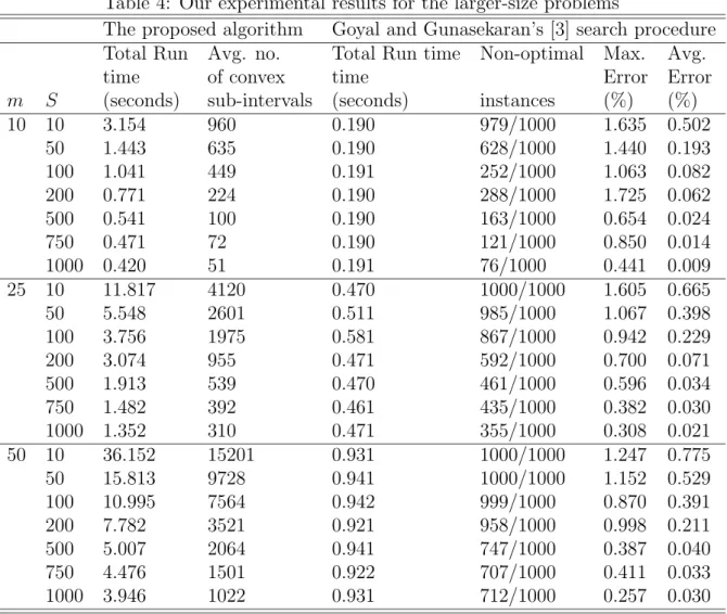
After randomly generating 42,000 instances in total, we solved each one of them by the proposed search algorithm as well as Goyal and Gunasekaran’s [3] search procedure on a Pentium-III PC with a 736M-CPU. Our experimental results for the smaller-size (withm = 3,5,7) and larger-size (with m= 10,25,50) are summarized in Tables 3 and 4, respectively. One may observe that the run time of Goyal and Gunasekaran’s [3] search procedure is extremely short. On the other hand, the proposed search algorithm solves the TFMSP with an optimal solution very efficiently. (We note that the third and the fourth columns
Table 2: The settings of the parameters in our random experiments m 3,5,7,10,25,50 S 10,50,100,200,500,750,1000 ni U[10−30] Xi U[0.4−0.8] Yi U[0.9−0.95] ai U[5−10] bi U[1−3] si U[25−40]
Table 3: Our experimental results for the smaller-size problems
The proposed algorithm Goyal and Gunasekaran’s [3] search procedure
m S Total Run Avg. no. Total Run Non-optimal Max. Avg.
time of convex time Error Error
(seconds) sub-intervals (seconds) instances (%) (%)
3 10 0.722 280 0.070 457/1000 3.673 0.268 50 0.320 80 0.080 174/1000 2.803 0.114 100 0.260 42 0.060 115/1000 2.138 0.056 200 0.191 23 0.060 65/1000 2.079 0.031 500 0.150 11 0.080 10/1000 0.318 0.014 750 0.130 8 0.060 1/1000 0.247 0.000 1000 0.130 7 0.060 2/1000 0.361 0.000 5 10 1.252 433 0.100 741/1000 2.363 0.366 50 0.571 152 0.091 288/1000 2.735 0.129 100 0.440 112 0.110 212/1000 1.796 0.089 200 0.321 67 0.090 148/1000 1.488 0.043 500 0.260 30 0.100 43/1000 1.244 0.009 750 0.211 18 0.100 20/1000 0.803 0.004 1000 0.190 15 0.100 6/1000 0.373 0.001 7 10 1.903 471 0.131 889/1000 1.862 0.449 50 0.891 295 0.140 470/1000 1.602 0.167 100 0.651 202 0.130 236/1000 1.381 0.070 200 0.491 104 0.150 203/1000 1.405 0.054 500 0.360 56 0.140 84/1000 0.723 0.015 750 0.311 37 0.141 46/1000 0.485 0.006 1000 0.270 28 0.140 32/1000 0.395 0.004
Table 4: Our experimental results for the larger-size problems
The proposed algorithm Goyal and Gunasekaran’s [3] search procedure Total Run Avg. no. Total Run time Non-optimal Max. Avg.
time of convex time Error Error
m S (seconds) sub-intervals (seconds) instances (%) (%)
10 10 3.154 960 0.190 979/1000 1.635 0.502 50 1.443 635 0.190 628/1000 1.440 0.193 100 1.041 449 0.191 252/1000 1.063 0.082 200 0.771 224 0.190 288/1000 1.725 0.062 500 0.541 100 0.190 163/1000 0.654 0.024 750 0.471 72 0.190 121/1000 0.850 0.014 1000 0.420 51 0.191 76/1000 0.441 0.009 25 10 11.817 4120 0.470 1000/1000 1.605 0.665 50 5.548 2601 0.511 985/1000 1.067 0.398 100 3.756 1975 0.581 867/1000 0.942 0.229 200 3.074 955 0.471 592/1000 0.700 0.071 500 1.913 539 0.470 461/1000 0.596 0.034 750 1.482 392 0.461 435/1000 0.382 0.030 1000 1.352 310 0.471 355/1000 0.308 0.021 50 10 36.152 15201 0.931 1000/1000 1.247 0.775 50 15.813 9728 0.941 1000/1000 1.152 0.529 100 10.995 7564 0.942 999/1000 0.870 0.391 200 7.782 3521 0.921 958/1000 0.998 0.211 500 5.007 2064 0.941 747/1000 0.387 0.040 750 4.476 1501 0.922 707/1000 0.411 0.033 1000 3.946 1022 0.931 712/1000 0.257 0.030
of Tables 3 and 4 indicate the total run time for all of the 1,000 instances for a particular parameter setting.) It takes less than36 seconds for 1,000 instances of larger-size problems with m = 50. (Or, we could solve each instance within 0.04 seconds on average.) For the readers’ further information on the run time, we also include the data of the average number of convex sub-intervals visited by the proposed algorithm in Tables 3 and 4.
On the aspect of solution quality, the proposed search algorithm significantly outperforms Goyal and Gunasekaran’s search procedure. In the fifth column of Tables 3 and 4, we indicate the number of instances out of the 1,000 instances in the combination ofmandSthat Goyal and Gunasekaran’s search procedure is not able to obtain an optimal solution. The number of instances that Goyal and Gunasekaran’s search procedure obtains non-optimal solutions increases as the size of the problemmincreases, and it decreases as the value ofS increases. In the last two columns of Tables 3 and 4, we present the maximum error and the average error of Goyal and Gunasekaran’s search procedure in percentages, respectively. We observe that the smaller the values ofmandS, the larger the maximum error and the average error. For the same value of S,the maximum error and the average error increase as the value of m increases. Also, for the same value of m, the average error decreases as the value of S increases.
6. Concluding Remarks
In this study, we presented a full analysis on the mathematical model for the Transportation Fleet Maintenance Scheduling Problem (TFMSP). We showed that the optimal objective function value of the mathematical model is piece-wise convex with respect toT. By utilizing our theoretical results, we proposed an efficient search algorithm that solves the optimal so-lution for the problem (P) within a very short run time. Based on our random experiments, we conclude that the proposed search algorithm out-performs Goyal and Gunasekaran’s [3] search procedure. Therefore, the proposed search algorithm provides the decision makers in transportation industries an excellent decision-support tool for their planned maintenance operations.
On the other hand, as one may notice it from our numerical results, the run time of the proposed algorithm grows significantly when the number of groups of vehicles (i.e., m) is large and the fixed maintenance cost (i.e., S) is small. The authors are currently devoting their efforts to improve the efficiency of the proposed algorithm for these cases.
Acknowledgement This research was supported by the National Science Council of Taiwan, ROC under Grant No. NSC 94-2213-E-029-014.
References
[1] M.S. Bazaraa and H.D. Sherali and C.M. Shetty: Nonlinear Programming: Theory and Algorithms, 2nd Ed. (John Wiley & Sons, New York, 1993).
[2] A.H. Christer and T. Doherty: Scheduling overhauls of soaking pits. Operational Re-search Quarterly,28 (1977), 915-926.
[3] S.K. Goyal and A. Gunasekaran: Determining economic maintenance frequency of a transportation fleet. International Journal of Systems Science,23 (1992), 655-659. [4] S.K. Goyal and M.I. Kusy: Determining economic maintenance frequency for a family
of machines. Journal of the Operational Research Society,36 (1985), 1125-1128. [5] R. Horst and P.M. Pardalos: Handbook of Global Optimization (Kluwer Academic
Publishers, Dordrecht, 1995).
[6] H. Luss: Maintenance policies when deterioration can be observed by inspections. Operations Research, 24 (1976), 359-366.
[7] H. Luss and Z. Kander: Preparedness model dealing with n systems operating simul-taneously. Operations Research,22 (1974), 117-128.
[8] D.R. Sule and B. Harmon: Determination of coordinated maintenance scheduling fre-quencies for a group of machines. AIIE Transactions, 11 (1979), 48-53.
[9] R. van Egmond, R. Dekker and R.E. Wildeman: Correspondence: determining eco-nomic maintenance of a transportation fleet. International Journal of Systems Science,
26 (1995), 1755-1757.
[10] S. Yanagi: Iteration method for reliability evaluation for a fleet system. Journal of the Operational Research Society, 43 (1992), 885-896.
Ming-Jong Yao
Department of Industrial Engineering and Enterprise Information,
Tunghai University,
180 , Sec. 3, Taichung Port Rd., Taichung City, 407 Taiwan, R.O.C.

![Table 2: The settings of the parameters in our random experiments m 3, 5, 7, 10, 25, 50 S 10, 50, 100, 200, 500, 750, 1000 n i U [10 − 30] X i U [0.4 − 0.8] Y i U [0.9 − 0.95] a i U [5 − 10] b i U [1 − 3] s i U [25 − 40]](https://thumb-us.123doks.com/thumbv2/123dok_us/9764616.2859427/13.892.112.777.529.1091/table-settings-parameters-random-experiments-s-u-x.webp)