Forecasting electronic part procurement lifetimes to enable the
management of DMSMS obsolescence
P. Sandborn
a,*, V. Prabhakar
a,
O. Ahmad
baCALCE Electronic Products and Systems Center, Department of Mechanical Engineering, University of Maryland,
College Park, MD 20742
b
SiliconExpert Technologies, Inc., 3375 Scott Blvd, Suite 406, Santa Clara, CA 95054
ABSTRACT
Many technologies have life cycles that are shorter than the life cycle of the product or system they are in. Life cycle mismatches caused by the obsolescence of technology can result in large life cycle costs for long field life systems, such as aircraft, ships, communications infrastructure, power plant and grid management, and military systems. This paper addresses DMSMS (Diminishing Manufacturing Sources and Materials Shortages) obsolescence, which is defined as the loss of the ability to procure a technology or part from its original manufacturer. Forecasting when technologies and specific parts will become unavailable (non-procurable) is a key enabler for pro-active DMSMS management and strategic life cycle planning for long field life systems. This paper presents a methodology for generating algorithms that can be used to predict the obsolescence dates for electronic parts that do not have clear evolutionary parametric drivers. The method is based on the calculation of procurement lifetime using databases of previous obsolescence events and introduced parts that have not gone obsolete. The methodology has been demonstrated on a range of different electronic parts and for the trending of specific part attributes.
*
Corresponding Author.
1. Introduction
For many high-volume, consumer oriented, fast-cycle products; a rapid rate of technology change translates into a need to stay on the leading edge of technology. These sectors seek to adapt the newest materials, components, and processes into their products in order to prevent loss of their market share to competitors. For products such as cell phones, digital cameras and laptop computers, evolving the design of a product or system is a question of balancing the risks of investing resources in new, possibly immature technologies against potential functional or performance gains that could differentiate them from their competitors in the market.
There are however, a number of product sectors that find it especially difficult to adopt leading-edge technology. Examples include: airplanes, ships, military systems, telecommunications infrastructure, computer networks for air traffic control and power grid management, industrial equipment, and medical equipment. These product sectors often “lag” in their adoption of new technology in part because of the high costs and/or long times associated with new product development. There are also significant roadblocks to modifying, upgrading and maintaining these systems over long periods of time because many of these products are “safety critical,” which means that lengthy and very expensive qualification/certification cycles may be required even for minor design changes. As a result, the manufacturers and customers of many of these products are more focused on sustaining1 the products for long periods of time (often 20 years or more) than upgrading them.
Trends in technology lifetimes and particularly electronic parts are important to organizations that must perform the long-term sustainment of their systems. The rapid rate of change in electronics poses significant challenges to industry sectors that must utilize electronics in long support life applications.
1
In this context sustainment refers to technology sustainment, i.e., the activities necessary to: a) keep an existing product operational (able to successfully complete its intended purpose); b) continue to manufacture and field versions of the system that satisfy the original requirements; and c) manufacture and field revised versions of the
This paper is organized as follows. In Section 2 we define DMSMS type technology obsolescence. Section 2 also describes the state-of-the-art in forecasting DMSMS obsolescence. In Section 3 we present a new methodology for procurement lifetime forecasting and demonstrate its application to various types of electronic parts for obsolescence forecasting. Finally, we summarize our results in Section 4 and discuss the forecasting methodology’s limitations.
2. DMSMS type technology obsolescence
Technology obsolescence is defined as the loss or impending loss of original manufacturers of items or suppliers of items or raw materials [2]. The type of obsolescence described in Section 1 and addressed in this paper is referred to as DMSMS (Diminishing Manufacturing Sources and Material Shortages) and is caused by the unavailability of technologies (parts) that are needed to manufacture or sustain a product.2 DMSMS means that due to the length of the system’s manufacturing and support life, coupled with unforeseen life extensions to support the system, needed parts become unavailable (or at least unavailable from their original manufacturer). Obsolescence is one of a number of part change and part supply chain problems that complicate the management of electronic systems, [4].
The fundamental disparities in life cycle needs and business objectives impose inevitable obsolescence challenges. Many long field life products particularly suffer the consequences of electronic part obsolescence because they have no control over their electronic part supply chain due to their relatively low production volumes. DMSMS type obsolescence occurs when long field life systems must depend on a supply chain that is organized to support high-volume products. Obsolescence becomes a problem when it is forced upon an organization; in response, that organization may have to involuntarily
2
Inventory or sudden obsolescence, which is more prevalent in the operations research literature, refers to the opposite problem to DMSMS obsolescence in which inventories of parts become obsolete because the product or system they were purchased for changes so that the inventories are no longer required, e.g., [3].
make a change to the product that it manufactures, supports or uses.3 Fig. 1 shows that magnitude of the problem today. The 1.1 million electronic part discontinuances in 2009 represents approximately 0.9% of the electronic parts available in the market.4
The majority of DMSMS obsolescence management today is reactive in nature – managing problems after they occur using a mixture of the mitigation approaches that include [6]: lifetime buy, last-time buy, aftermarket sources, identification of alternative or substitute parts, emulated parts, salvaged parts, and thermal uprating [7]. Potentially larger cost avoidances are possible with pro-active and strategic management approaches, [8]. Pro-active management means identifying and prioritizing selected non-obsolete parts that are at risk of obsolescence and identifying resolutions for them before they are discontinued. Design refreshes ultimately occur as other mitigation options are exhausted and functionality upgrades (technology insertion) becomes necessary. Strategic management is done in
3
Researchers who study product-development characterize different industries using the term “clockspeed,” which is a measure of the dynamic nature of an industry, [5]. The type of industries that generally deal with DMSMS problems would be characterized as slow clockspeed industries. In addition, because of the expensive nature of the products (e.g., airplanes, ships, etc.) the customers can’t afford to replace these products with newer versions very often (i.e., slow clockspeed customers). DMSMS type obsolescence occurs when slow clockspeed industries must depend on a supply chain that is organized to support fast clockspeed industries.
4
As of June 2010 SiliconExpert Technologies’ parts database consisted of approximately 157.2 million unique parts (approximately 121.6 million of which are not obsolete). Part count includes all derivations of part numbers based
0 200,000 400,000 600,000 800,000 1,000,000 1,200,000 1,400,000 1,600,000 2006 2007 2008 2009 P ro d u c t D is c o n ti n u a n c e N o ti c e s
Fig. 1. The total number of product discontinuance notices (notices from the original manufacturer that manufacturing of the part will be terminated) for electronic parts in years 2006-2009 from SiliconExpert Technologies, Inc. databases.
addition to pro-active and reactive management, and involves the determination of the optimum mix of mitigation approaches and design refreshes, [9].
The key enabler for pro-active and strategic management of DMSMS obsolescence is the ability to forecast the obsolescence events for key parts. The remainder of this paper addresses forecasting DMSMS obsolescence.
2.1. DMSMS obsolescence forecasting
Obsolescence forecasting strategies can be broken into two types of forecasts. Long-term forecasts that are used when obsolescence is one year or further into the future to enable pro-active management of obsolescence events and strategic life cycle planning for the sustainment of systems. The second type of forecasting is short term. Short-term forecasting observes the supply chain for precursors to a part’s obsolescence. Precursors can include reduction in the number of sources that a part is available from, reductions in distributor inventories of the part, price increases that may in some cases accompany a reduction in the availability of the part, and/or announcements made by the part manufacturers that indicate either directly or indirectly that the part is being phased out.
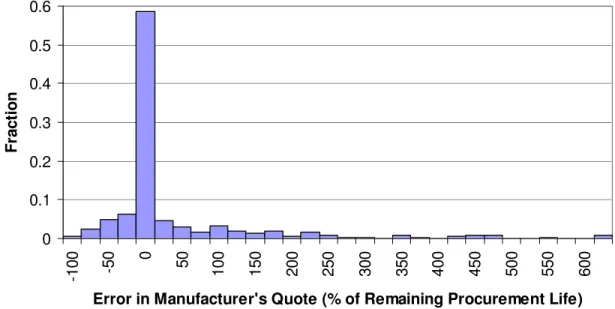
Common strategies use long-term obsolescence forecasting while continuously monitoring the supply chain for precursors to obsolescence. This strategy abandons the long-term forecast when a combination of subjective indicators of discontinuance associated with a part are observed. In itself, the lack of precursors only indicates that discontinuance of the part is likely to be more than one year in the future, therefore, the supply chain indicators (precursors) are not generally useful for forecasting the long-term availability of the part. The remainder of this paper focuses on the long-term forecasting of obsolescence. The most straightforward approach to forecasting obsolescence (either short or long term) is to simply ask the manufacturer of the part when the part will be discontinued. Fig. 2 was created using the results of a survey of electronic parts conducted in [10] and indicates the frequency of over and under prediction of procurement life by manufacturers. Using the survey results, the error was calculated using,
− − − =100 1 inquiry MQO inquiry O D D D D Error (1) where
DO = Obsolescence date, the date that the manufacturer actually discontinued the part
Dinquiry = The date that the inquiry was made with the manufacturer
DMQO = Manufacturer’s quoted obsolescence date.
The survey showed that 58.7% of manufacturer’s obsolescence quotes are accurate and that actual obsolescence dates are more likely to occur later than the manufacturer-quoted date (25..6% after) than before it (15.7% before). On average, the remaining production time is 35% longer than that promised by the manufacturers, however, in this survey 1.5% of manufacturers incorrectly stated that their own parts were still in production when in fact they were already discontinued. Fig. 2 shows the results for just manufactures that responded to the survey, manufacturers realize that their responses to customers regarding the procurement outlook for a part can become self-fulfilling prophecies and may therefore be hesitant to provide information to customers who may be purchasing relatively small volumes of parts.
0 0.1 0.2 0.3 0.4 0.5 0.6 -1 0 0 -5 0 0 50 1 0 0 1 5 0 2 0 0 2 5 0 3 0 0 3 5 0 4 0 0 4 5 0 5 0 0 5 5 0 6 0 0
Error in Manufacturer's Quote (% of Remaining Procurement Life)
F ra c ti o n
Fig. 2. Accuracy of manufacturer quoted obsolescence dates. Zero indicates an accurate quote. To the left of zero, the part was discontinued earlier than the manufacturer’s quote; to the right of zero the part was discontinued later than the manufacturer’s quote.
Due to an inability to obtain manufacturer obsolescence date estimates coupled with the lack of accuracy when estimates are obtained, alternative types of forecasting that do not depend on the manufacturer are also used.
Most long-term electronic part obsolescence forecasting5 is based on the development of models for the part’s life cycle. Traditional methods of life cycle forecasting are ordinal scale based approaches, in which the life cycle stage of the part is determined from a combination of technological and supply chain attributes such as level of integration, minimum feature size, type of process, number of sources, etc., e.g., [12-14], and those available in several commercial databases. The ordinal scale based approaches work best as short-term forecasts, but their accuracy in the long-term has not been quantified. For ordinal scale approaches the historical basis for forecasts is subjective and confidence levels and uncertainties are not generally evaluatable. To improve forecasting, more general models based on technology trends have also appeared including a methodology based on forecasting part sales curves, [15,16], and leading-indicator approaches [17,18]. A method based on data mining the historical record that extends the part sales curve forecasting method and which is capable of quantifying uncertainties in the forecasts has also been developed, [19]. Gravier and Swartz [20], present a general statistical study of a set of 235 parts drawn from a cross section of IC functions, technologies and voltage levels to determine the probability of no suppliers (effectively the probability of obsolescence) as a function of the years since the introduction of the part.
Existing commercial forecasting tools are good at articulating the current state of a part’s availability and identifying alternatives, but are limited in their capability to forecast future obsolescence dates and do not generally provide quantitative confidence limits when predicting future obsolescence dates or risks. Pro-active and strategic obsolescence management approaches require more accurate forecasts or at least forecasts with a quantifiable accuracy. Better part-specific forecasts with uncertainty estimates would
5
DMSMS obsolescence forecasting is a form of product deletion modeling, e.g., [11], that is performed without inputs from or the cooperation of the part manufacturer.
open the door to the use of life cycle planning tools that could lead to more significant sustainment cost avoidance, [9].
3. Procurement lifetime forecasting
Previously proposed data mining methods for forecasting obsolescence [19] have been shown to work well when there are identifiable evolutionary parametric drivers. An evolutionary parametric driver is a parameter (or a combination of parameters) describing the part that evolve over time. For example, for flash memory chips an evolutionary parametric driver is memory size, traditionally for microprocessors it has been clock frequency (although recently this has begun to give way to power consumption). Unfortunately, for the majority of electronic parts, there is no simple evolutionary parametric driver that can be identified and previously proposed data mining approaches cannot be used.
In this section we present a methodology for formulating obsolescence forecasting algorithms based on predicting the part’s procurement life that does not depend on the identification of an evolutionary parametric driver for the part. The procurement life for a part is defined as,
I O P D D
L = − (2)
where
LP = Procurement life, amount of time the part was (or will be) available for procurement from its original manufacturer
DO = Obsolescence date, the date that the original manufacturer discontinued or will discontinue the part
DI = Introduction date, the date that the original manufacturer introduced the part.
The concept of procurement life has also been referred to as “product lifetime” by [21] and “duration time” in the marketing literature, e.g., [22]. In this paper we are interested in exploring the correlation between procurement lifetime and introduction date for electronic parts. Two specific results are of
interest for forecasting uses: first the mean procurement lifetime as a function of introduction date (Section 3.2) and second the effective worst case procurement lifetime as a function of introduction date (Section 3.3). Before discussing these forecasts, we briefly describe the data used in this analysis.
3.1. Electronic part introduction date and obsolescence date data
A part database from SiliconExpert was used for the analysis in this paper. The part database was created and is maintained using parts data that is sourced via web crawling of manufacturers’ websites for revision control and through direct relationships with manufacturers where feeds of component data are supplied on a weekly, monthly or quarterly basis. The frequency of updates is dependent upon how often datasheets and product information are revised by document controllers internally at each manufacturer. In addition, data feeds provided via direct relationships enlist datasheets and parametric information for new products introduced to the market. Organization of the database is done through a strict taxonomy. Revisions to the taxonomy occur only for expansion and contraction of existing product lines to ensure valid differentiation between various subcategories. As of June 2010, the database contained over 157 Million electronic parts spanning 337 product lines from 11,054 manufacturers.
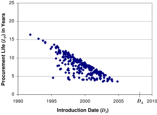
Fig. 3 shows an example plot of procurement life versus introduction date for obsolete linear regulators (a common electronic part that is a voltage regulator placed between a supply and the load and provides a constant voltage by varying its effective resistance) mined from the SiliconExpert database described above.
3.2. Determining mean procurement lifetimes
The mean procurement lifetimes for parts can be analyzed using the statistical framework for failure time analysis [22]. This approach has been previously used to determine the mean product life cycle
lengths for personal computers, [21]. The approach in [21] and [22], however, has never been applied to the forecasting of obsolescence or to the procurement of electronic parts.
The event of interest in this paper is the discontinuance (obsolescence) of an instance of a part. The data used (e.g., Fig. 3) includes the introduction dates of all the parts of a particular type and the obsolescence dates for the parts that have occurred up to 2008. An obsolescence event is not observed for every part in the data set since some of the introduced parts had not gone obsolete as of the analysis date, i.e., the observations are right censored.
Following the analysis method in [22] and representing the data for the linear regulator example shown in Fig. 3 as a distribution of procurement lifetimes (event density), f(t), with a corresponding cumulative distribution function, F(t), the hazard rate, h(t) is given by,
) ( 1 ) ( ) ( t F t f t h − = (3) 0 5 10 15 20 25 1990 1995 2000 2005 2010 Introduction Date P ro c u re m e n t L if e ( y e a rs ) Introduction Date (DI) P ro c u re m e n t L if e ( LP ) in Y e a rs DA
Fig. 3. 347 obsolete linear regulators from 33 manufacturers. DA = 2008, the analysis date (the date on
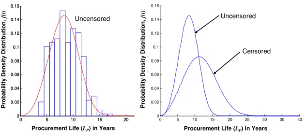
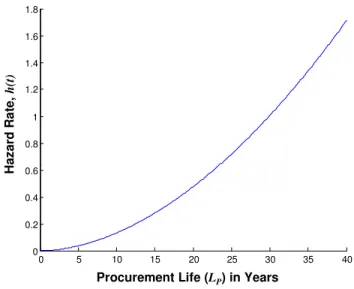
The hazard rate is the probability that a part will become non-procurable at time t assuming it was procurable in the interval (0,t). Fig. 4 shows f(t) and the corresponding hazard rate, h(t) for linear regulators is shown in Fig. 5. To determine f(t) the data was fit with a 2-parameter Weibull,
β η β η η β − − = t e t t f 1 ) ( (4)
where the parameters were estimated using MLE (Maximum Likelihood Estimation) assuming right censoring and that the censoring mechanism is non-informative (the knowledge that the observation is censored does not convey any information except that the obsolescence dates of some parts within the data set lie beyond the censoring date, which is the analysis date (DA) in our case).
6
In Fig. 4, the uncensored distribution ignores the introduced parts that had not gone obsolete as of DA. Obviously, the mode is shifted to the left (smaller procurement lifetimes) when the non-obsolete parts are ignored. In the case of linear regulators, the hazard rate shown in Fig. 5 increases with time (dh(t)/dt > 0), indicating that the longer the procurement lifetime, the more likely the part is to go obsolete. In the case of the linear regulators, there are 347 obsolescence events out of a total of 847 introduced parts.
6
The MLE parameter estimation was performed using the MatLAB Statistics package.
0 5 10 15 20 25 30 0 0.02 0.04 0.06 0.08 0.1 0.12 0.14 0.16 Uncensored P ro b a b ili ty D e n s it y F u n c ti o n Procurement Life
Procurement Life Data Uncensored - Weibull (2-P) P ro b a b il it y D e n s it y D is tr ib u ti o n , f( t)
Procurement Life (LP) in Years
0 5 10 15 20 25 30 0 0.02 0.04 0.06 0.08 0.1 0.12 0.14 0.16 Uncensored P ro b a b ili ty D e n s it y F u n c ti o n Procurement Life
Procurement Life Data Uncensored - Weibull (2-P) P ro b a b il it y D e n s it y D is tr ib u ti o n , f( t)
Procurement Life (LP) in Years
0 5 10 15 20 25 30 35 40 0 0.02 0.04 0.06 0.08 0.1 0.12 0.14 0.16 P ro b a b ili ty D e n s it y D is tr ib u ti o n Procurement Life Censored Uncensored
Procurement Life (LP) in Years
P ro b a b il it y D e n s it y D is tr ib u ti o n , f( t) Uncensored
Fig. 4. The distribution of procurement lifetimes for linear regulators. The histogram on the left side corresponds to the data in Fig. 3. The mean procurement lifetime (censored) = 11.63 years, β = 2.84, η = 13.06. The parameters are based on a maximum likelihood estimate (MLE) using a two-parameter Weibull fit.
Fig. 6 shows the quantity and fraction of non-obsolete linear regulators as a function of time. This plot shows that a large fraction of the parts introduced in 1990-1996 have not gone obsolete yet (but the total number introduced during this period is also relatively small). An alternative way to look at this is to perform the analysis described above for determining the mean procurement lifetime on the data set as a function of time (Fig. 7). In this case, to generate the mean procurement lifetime at a particular date (or before), we only consider the parts that had been introduced on or before that date in the analysis (although all observations are made in 2008). The mean procurement life is analogous to the mean time-to-failure (MTTF). The mean procurement life for a given Weibull distribution can be calculated using,
+ = β Γ η 1 t Lp (5)
where β and η are the Weibull parameters corresponding to the data fits up to DI.
H a z a rd R a te , h (t ) 0 5 10 15 20 25 30 35 40 0 0.2 0.4 0.6 0.8 1 1.2 1.4 1.6 1.8
Procurement Life (LP) in Years
Fig. 5. Hazard rate corresponding to the censored distribution of procurement lifetimes for linear regulators in Fig. 4.
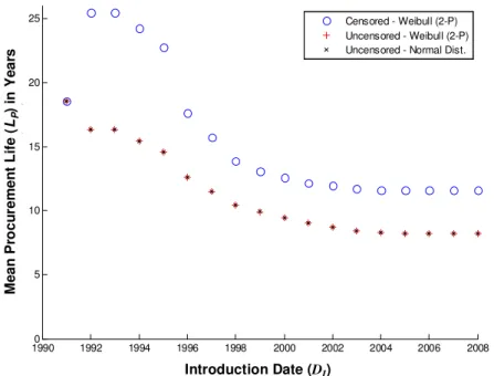
Fig. 7 indicates the appropriate mean procurement lifetime to assume for parts with introduction dates at or before the indicated year. So a part introduced in 1998 or before has a mean procurement lifetime of 14 years (Censored – Weibull (2-P) in Fig. 7). In order to determine the mean procurement lifetime for parts introduced in a particular year (rather than in or before a particular year), “slices” of the data must be used. In this case, to generate the mean procurement lifetime at a particular date, we only consider the parts that have been introduced within one year periods in the analysis and once again, all observations are made in 2008. Fig. 8 shows the mean procurement lifetimes for one year slices with and without right censoring assuming that we are observing in 2008. For example, for a part introduced in 1998, Fig. 8 predicts that the mean procurement lifetime will be 11.5 years (smaller than the 14 years predicted by Fig. 7). Fig. 8 and the comparison of Figs. 7 and 8 indicate that older linear regulators (smaller DI) have longer procurement lifetimes (LP) than newer linear regulators.
Using the data from Fig. 8 for 1990-2005 (excluding 1993 since no parts were introduced in 1993), the mean procurement life trend is given by,
7 . 86095 2217 . 85 021089 . 0 2 − + = I I p D D L (6) 0 100 200 300 400 500 600 1991 1993 1995 1997 1999 2001 2003 2005 2007 Introduciton Date N u m b e r o f P a rt s t h a t a re N o t O b s o le te 0.5 0.55 0.6 0.65 0.7 0.75 0.8 0.85 0.9 0.95 1 F ra c ti o n o f P a rt s t h a t a re N o t O b s o le te
Number of Parts (left axis) Fraction of Parts (right axis)
Introduction Date (DI)
The analysis in this section provides a useful estimation of the mean procurement lifetime for parts, however, the worst case procurement lifetimes are also of interest to organizations performing pro-active
M e a n P ro c u re m e n t L if e ( Y e a rs ) Introduction Date (DI) 19900 1992 1994 1996 1998 2000 2002 2004 2006 2008 5 10 15 20 25 Censored - W eibull (2-P) Uncensored - Weibull (2-P) Uncensored - Normal Dist.
M e a n P ro c u re m e n t L if e ( LP ) in Y e a rs
Fig. 8. Mean procurement lifetime for linear regulators as a function of time (parts introduced on the date). Note, there were no parts introduced in 1993.
19900 1992 1994 1996 1998 2000 2002 2004 2006 2008 5 10 15 20 25 Year M e a n P ro c u re m e n t L if e ( Y e a rs ) Censored - Weibull (2-P) Uncensored - Weibull (2-P) Uncensored - Normal Dist.
Introduction Date (DI) M e a n P ro c u re m e n t L if e ( LP ) in Y e a rs
Fig. 7. Mean procurement lifetime for linear regulators as a function of time (parts introduced on or before the date).
and strategic DMSMS obsolescence management. The next section provides a more detailed interpretation of the procurement life versus introduction date profiles (e.g., Fig. 3) and discusses the generation of worst case forecasts.
3.3. An interpretation of procurement life and worst case forecasts
Several distinct regions on the graph in Fig. 3 can be identified. The upper bound of where specific data points (corresponding to specific observed obsolescence events) can lie in Fig. 3 is given by LP = DA -DI, where DA is the analysis date, i.e., the date the analysis was performed on (in Fig. 3, DA is 2008). The data set of known (observed) obsolescence events must always lie on or below this line. The region above this line represents parts that were introduced in the past but are not obsolete yet. The region defined by
DI > DA could be populated by future part introductions. If the data set is complete (i.e., all parts that
have gone obsolete up to DA are included in the data set) then the region below the data and to the left of the LP = DA-DI line will be empty.
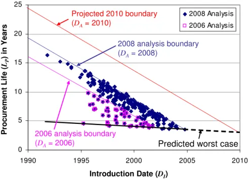
The top boundary of the procurement life versus introduction date plot changes with the addition of future obsolescence events, but the bottom boundary of the data sets tends to stay constant over time as data is added. This is shown in Fig. 9 where the 2008 analysis data includes all the obsolescence events that have occurred to date, the 2006 data includes all linear regulators that were introduced in 2006 or before and were obsolete in 2006 or before, and the projected 2010 analysis boundary is shown. In this case, the bottom boundary for parts introduced after 2005 is not known but can be projected based on the historical trend.
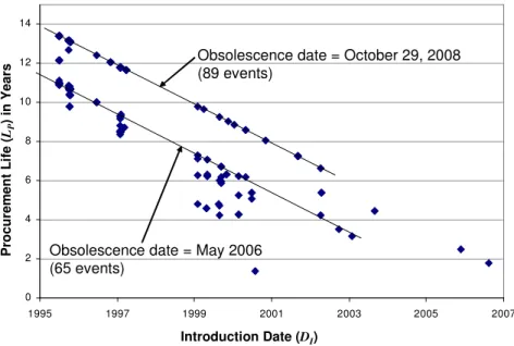
The top boundary of the data shown in Fig. 3 will always have a slope of -1 because it is generated by a group of parts introduced on various dates that are all discontinued on or about the same date,7 which is a common practice for electronic parts manufacturers, see Fig. 10. A group of parts all having the same procurement life that are introduced on various dates would produce a horizontal line of data points on the plot. A vertical line of data points on the plot indicates that the parts all have the same introduction date and various discontinuance dates.8
7
The upper bound is defined by parts whose obsolescence date is DA and therefore the slope of the upper bound is
given by, -(DA-DI)/(DA-DI) = -1.
8
In our experience, vertical lines of data points may be indicative of errors in the historical record. The most common error is that the introduction dates for the parts are the database record creation dates not the actual part
0 5 10 15 20 25 1990 1995 2000 2005 2010 Introduction Date P ro c u re m e n t L if e ( y e a rs ) 2008 Analysis 2006 Analysis Projected 2010 boundary (DA= 2010) 2008 analysis boundary (DA= 2008) 2006 analysis boundary
(DA= 2006) Predicted worst case
Introduction Date (DI) P ro c u re m e n t L if e ( LP ) in Y e a rs
The bottom boundary of the data shown in Fig. 3 is the key to forecasting the worst case procurement life. In cases where the “age” of the part (how long ago it was introduced) has no effect on the procurement life, the bottom boundary of the data set will be flat (slope = 0). If there is an age effect, the bottom boundary of the data set will have a non-zero slope. Parts with strong evolutionary parametric drivers have flat bottom boundaries. In the case of parts with strong evolutionary parametric drivers, the parametric driver usually causes the part to be discontinued before procurement age has any impact. Fig. 11 shows the procurement life versus introduction date for flash memory devices. The data set starts in late 1992 (earliest introduction dates), the bottom boundary of the data is flat; flash memory obsolescence is driven by the memory size, not by procurement age, i.e., see [19]. Alternatively, Fig. 12 shows the procurement life versus introduction date for operational amplifiers (“op amps”). This characteristic clearly shows that for op amps introduced prior to 1993 there was a strong age effect, starting in 1993 the age effect weakened but is still present.
0 2 4 6 8 10 12 14 1995 1997 1999 2001 2003 2005 2007 Introduction Date P ro c u re m e n t L if e ( y rs )
Obsolescence date = October 29, 2008 (89 events)
Obsolescence date = May 2006 (65 events) Introduction Date (DI) P ro c u re m e n t L if e ( LP ) in Y e a rs
For linear regulators shown in Fig. 3 the bottom boundary (worst case procurement lifetime) is given by, 5 . 4188 0947 . 2 + − = I P D L for DI≤ 1997.5 (7a) 77 . 206 1014 . 0 + − = I P D L for DI > 1997.5 (7b)
As indicated in Eq. (7), the linear regulator procurement life trends show two distinct aging regimes. Other part types also often have multiple aging regimes, e.g., operational amplifiers shown in Fig. 12. The exact reason for the discontinuity is not known, however, Fig. 6 shows that the year of the discontinuity for linear regulators (1997.5) is close to the minima in the fraction of parts that are not obsolete graph and in both the linear regulator and operation amplifier cases, the year of the discontinuity in the procurement life trend also corresponds to a period of slow growth rate for the semiconductor industry, see Fig. 13. Another possibility is that parts simply reach a minimum viable procurement life dictated by the high-volume products that demand the parts.
0.00 2.00 4.00 6.00 8.00 10.00 12.00 14.00 16.00 18.00 20.00 1992 1994 1996 1998 2000 2002 2004 2006 2008 Introduction Year P ro c u re m e n t L if e ( y e a rs ) Introduction Date (DI) P ro c u re m e n t L if e ( LP ) in Y e a rs
0 4 8 12 16 20 24 28 32 36 1969 1974 1979 1984 1989 1994 1999 2004 Introduction Year P ro c u re me n t L if e ti me ( y e a rs ) Introduction Date (DI) P ro c u re m e n t L if e ( LP ) in Y e a rs
Fig. 12. Operational amplifier devices (2400 total obsolescence events from 7 manufacturers).
-40% -30% -20% -10% 0% 10% 20% 30% 40% 50% 1980 1985 1990 1995 2000 2005 2010 2015 Year S e m ic o n d u c to ry I n d u s tr y G ro w th R a te Discontinuities in the procurement life trend
O p e ra ti o n a l A m p lif ie rs L in e a r R e g u la to rs
Fig. 13. Correlation of discontinuities in the procurement life trends with the semiconductor industry growth rate. (2007-2011 growth rates are forecasted) [23].
3.4. Part type specific results
The analysis described in Section 3.2 and Section 3.3 has been applied to a variety of electronic parts. Table 1 provides results for selected part types.
Table 1
Procurement lifetimes for various electronic part types through 2008. β and η refer to 2 parameter Weibull fits of the censored and uncensored PDFs. LKV is the negative log-likelihood function (larger negative values indicate a better fit).
Part Type Censored Uncensored % of
parts not obsolete Total number of parts Mean (years) β η LKV Mean (years) β η LKV Linear Regulators 11.63 2.842 13.06 -1205 8.245 3.470 9.168 -822 59.46% 509 Buffer & Line Drivers 38.39 2.021 43.33 -3042 9.821 4.008 10.83 -1293 91.08% 1279 Bus Transceivers 15.39 2.289 17.37 -1746 9.281 4.988 10.11 -984 57.26% 1057 Decoder & Demux 20.74 1.713 23.25 -914.9 9.298 4.505 10.19 -490 62.30% 565 Flip Flop 16.23 2.250 18.33 -1727 9.638 5.154 10.48 -950 58.27% 1052 Inverter Schmitt Trigger 18.13 1.830 20.40 -1125 8.575 4.061 9.453 -627 64.13% 750 Latch 14.99 2.289 16.92 -1391 9.186 4.952 10.01 -792 55.46% 818 Multiplexer 18.83 1.819 21.19 -844.0 8.835 4.096 9.734 -470 63.70% 552
The methodology described in this paper can also be applied to specific manufacturers as shown in Fig. 10 and Fig. 14. Fig. 14 shows the determination of the worst case obsolescence forecast as a function of introduction year for linear regulators manufactured by National Semiconductor. The methodology can also be applied to key attributes of parts. Fig. 15 shows a procurement lifetime plot for 5 volt bias logic parts. Fig. 15 is interesting because it clearly shows a decreasing procurement lifetime for parts introduced before 1999 (this is consistent with broad trend from 5 volt bias parts to lower voltages, e.g., 3.3 volts and lower), however, the results also indicate that this trend may have reversed for parts introduced after 1999. This trend does not indicate that electronic parts are changing from lower bias levels back to 5 volts; rather it shows that 5 volt parts introduced after 1999 are being supported longer than their predecessors that were phased out in favor of lower bias voltage versions were, i.e., manufacturers that introduce 5 volt parts now are targeting applications that are either not transitioning to lower voltage levels or whose conversion to lower voltage levels is slow.
0 2 4 6 8 10 12 14 16 18 20 1993 1995 1997 1999 2001 2003 2005 Introduction Date P ro c u re m e n t L if e ( y e a rs )
Worst case forecast for linear regulators from all manufacturers Worst case forecast for National Semiconductor linear regulators
Introduction Date (DI) P ro c u re m e n t L if e ( LP ) in Y e a rs
4. Discussion and conclusions
In this paper, we have presented a methodology for constructing algorithms that can be used to forecast the procurement lifetime, and thereby the obsolescence date, of technologies based on data mining the historical record. Unlike previous methods for forecasting DMSMS type obsolescence, this method is applicable to technologies that have no clear evolutionary parametric driver. Results from the methodology applied to several different electronic part types have been included.
Long range forecasting techniques generally involve methods of trend extrapolation. The worst case procurement life trend for the linear regulator example developed in this paper is shown on Fig. 9 and quantified in Eq. (7). Although, trending the worst case procurement lives should be done using just the uncensored data (only the obsolete parts), trends in the mean procurement life must be done using the censored data set (both obsolete and non-obsolete parts) from Fig. 8 corresponding to Eq. (6).
0 5 10 15 20 25 1985 1990 1995 2000 2005 2010 Introduction Date P ro c u re m e n t L if e ( y rs ) Procurement Life Decreasing before 1999 Procurement Life of 5V Logic Parts Increasing after 1999 Introduction Date (DI) P ro c u re m e n t L if e ( LP ) in Y e a rs
It has been suggested that the “age” of electronic parts is not necessarily a factor in determining what gets obsoleted, [24]. The age of a part can be interpreted two ways; either it represents how long ago the part was introduced (DA - DI) where DA is the analysis date (DA - DI is referred to as “design life” in [20]), or how long the part was procurable for (LP). The results in this paper suggest that age is a factor in predicting the obsolescence of the part for parts that do not have strong evolutionarily parametric drivers. Gravier and Swartz [20] also conclude that age is correlated to obsolescence by showing that the probability of no suppliers varies with design life. However [20] does not distinguish between part types (except for military and non-military parts) or part’s with or without strong evolutionary parametric drivers.
For the procurement lifetime forecasting algorithms developed using the methodology proposed in this paper to be useful, one must assume that past trends are a valid predictor of the future. In some cases, particular technologies or parts may be displaced by some unforeseen new disruptive technology, thus accelerating the obsolescence of the existing parts faster than what the historical record would forecast. Alternatively, new applications may appear that extend or create demand for specific technologies or parts also causing a change in the historical obsolescence patterns for the parts. Application of the proposed method depends on having access to sufficient historical data to support a statistical analysis; this is especially true when one wishes to refine the forecasts (to particular vendors or particular part attributes).
The obsolescence date of a part or technology from the original manufacturer may or may not be a critical date in the management of a product or system depending on how the part or technology is used. Original manufacturer obsolescence dates when combined with the forecasted future need for the part and the available inventory of the part determine whether the obsolescence of the part is a problem or not, or when the obsolescence of the part will become a problem. For example, minimum buy sizes for many inexpensive electronic parts (e.g., resistors and capacitors), may far exceed the number of parts needed to manufacture and support a low-volume product, so the obsolescence of the inexpensive part may be a non-issue because the available supply of parts will never be exhausted. For a high-volume product, the
quantity of parts needed may quickly exceed what can be supplied by the existing inventory of parts and aftermarket suppliers, so forecasting the original manufacturers’ obsolescence date is critical in order to enable strategic management of the product.
Forecasting procurement lifetime is important to more than just the management of long field life products. Decision making for the advanced technology oriented product development process must balance the possible shrinkage in procurement life of required component technologies against the need for thoroughness, quality, market share retention, and many other factors. Procurement life is a more readily available (and useful) measure of part and technology availability than obsolescence date. While obsolescence date forecasting for specific instances of parts (for specific part numbers) is an important driver for reactive management of DMSMS type obsolescence. For strategic management of DMSMS over a long sustainment period, it is often more useful to know the procurement life (the period of time that the original manufacturer sells the item or supports the item) than the obsolescence date of the particular instance of the item you currently have in your system. In strategic planning and management, the primary interest is in determining the optimum frequency of refresh and not necessarily the optimum management of the particular instance of the part that is in the system today.
References
[1] Sandborn P, Myers J. Designing engineering systems for sustainment. Handbook of performability engineering, KB Misra (Editor), Springer, London, 2008, pp. 81-103.
[2] Sandborn P. Trapped on technology’s trailing edge. IEEE Spectrum 2008; 45:42-45, 54, 56-58. [3] Brown G, Lu J, Wolfson R. Dynamic modeling of inventories subject to obsolescence,
Management Science 1964; 11:51-63.
[4] Murray S, Boru M, Pecht M. Tracking semiconductor part changes through the part supply chain. IEEE Trans. on Components and Packaging Technologies 2002; 25: 230-238.
[5] Fine C. Clockspeed: Winning industry control in the age of temporary advantage. Reading, MA: Perseus Books; 1998.
[6] Stogdill C. Dealing with obsolete parts. IEEE Design & Test of Computers 1999; 16:17-25. [7] Pecht M, Humphrey D. Uprating of electronic parts to address obsolescence. Microelectronics
International 2006; 23:32-36.
[8] Sandborn P. Strategic management of DMSMS in systems. DSP Journal 2008; 24-30.
[9] Singh P, Sandborn P. Obsolescence driven design refresh planning for sustainment-dominated systems. The Engineering Economist 2006; 51:115-139.
[10] Gaintner M. Analysis of end of production (EOP) and end of support (EOS) dates at the LRU level, NAVSEA Dam Neck; 2007.
[11] Avlonitis G, Hart S, Tzokas N. An analysis of product deletion scenarios. Journal of Product Innovation Management 2000; 17:41-56.
[12] Henke A, Lai S. Automated parts obsolescence prediction. In: Proceedings of the DMSMS Conference, 1997.
[13] Lai D. Automated parts obsolescence prediction In: Proceedings of the DMSMS Conference, 1997.
[14] Josias C, Terpenny J. Component obsolescence risk assessment. In: Proceedings of the Industrial Engineering Research Conference (IERC), 2004.
[15] Solomon R, Sandborn P, Pecht M. Electronic part life cycle concepts and obsolescence forecasting. IEEE Trans. on Components and Packaging Technologies 2000; 23:707-713. [16] Pecht M, Solomon R, Sandborn P, Wilkinson C, Das D. Life Cycle Forecasting, Mitigation
Assessment and Obsolescence Strategies, CALCE EPSC Press, 2002.
[17] Meixell M, Wu S. Scenario analysis of demand in a technology market using leading indicators. IEEE Transactions on Semiconductor Manufacturing 2001; 14:65-78.
[18] Wu S, Aytac B, Berger R. Managing short life-cycle technology products for Agere Systems. Interfaces 2006; 36:234-247.
[19] Sandborn P, Mauro F, Knox R. A data mining based approach to electronic part obsolescence forecasting. IEEE Transactions on Components and Packaging Technologies 2007; 30:397-401. [20] Gravier, M, Swartz, S. The dark side of innovation: Exploring obsolescence and supply chain evolution for sustainment-dominated systems. Journal of High Technology Management Research 2009; 20:87-102.
[21] Bayus B. An analysis of product lifetimes in a technologically dynamic industry. Management Science 1998; 44:763-775.
[22] Helsen K, Schmittlein D. Analyzing duration times in marketing: Evidence for the effectiveness of hazard rate models. Marketing Science 1993; 11:395-414.
[23] McClean Report, IC Insights, Inc., 2007.