Spatial Mass Spectral Data
Analysis Using Factor and
Correlation Models
Lingli Shen
Thesis submitted for the Degree of Doctor of Philosophy Department of Automatic Control and Systems Engineering
The University of Sheffield March 2015
Abstract
ToF-SIMS is a powerful and information rich tool with high resolution and sensitivity compared to conventional mass spectrometers. Recently, its application has been extended to metabolic profiling analysis. However, there are only a few algorithms currently available to handle such output data from metabolite samples. Therefore some novel and innovative algorithms are undoubtedly in need to provide new insights into the application of ToF-SIMS for metabolic profiling analysis. In this thesis, we develop novel multivariate analysis techniques that can be used in processing ToF-SIMS data extracted from metabolite samples.
Firstly, several traditional multivariate analysis methodologies that have previously been suggested for ToF-SIMS data analysis are discussed, including Clustering, Principal Components Analysis (PCA), Maximum Autocorrelation Factor (MAF), and Multivariate Curve Resolution (MCR). In particular, PCA is selected as anexample to show the performance of traditional multivariate analysis techniques in dealing with large ToF-SIMS data extracted from metabolite samples. In order to provide more realistic and meaningful interpretation of the results, Non-negative Matrix Factorisation (NMF) is presented. This algorithm is combined with the Bayesian Framework to improve the reliability of the results and the convergence of the algorithm. However, the iterative process involved leads to considerable computational complexity in the estimation procedure.
Another novel algorithm is also proposed which is an optimised MCR algorithm within alternating non-negativity constrained least squares (ANLS) framework. It provides a more simpleapproximation procedure by implementing a dimensionality reduction based on a basis function decomposition approach. The novel and main feature of the proposed algorithm is that it incorporates a spatially continuous representation of ToF-SIMS data which decouplesthe computational complexity of
the estimation procedure from the image resolution. The proposed algorithm can be used as an efficient tool in processing ToF-SIMS data obtained from metabolite samples.
Acknowledgements
Four years ago I decided to begin the biggest challenge of my life, to study for a PhD program in engineering, I was so passionate at the beginning until bad things kept hitting me since three years ago. But luckily I have made it here to the end, I feel fulfilled no matter what the result will be, I am very fortunate that I have met so many nice people, who have stood by me to face the bad things during this challenging time.
Here I want to give my whole respect to one person, Professor Visakan Kadirkamanathan, who is not only my supervisor on this program, but also a mentor for my life. I made it to the end as one better and stronger person mostly because of his guidance. What he has given to me is not only the professional academic advice, but also the suggestions that has helped me through each barrier in my life. He is the one who has told me never give up when I wanted to, has told me life is not only about gaining the results, has told me that sometimes losing one thing doesn’t mean that you lose your whole life. Thank you, sir, for everything, without you, I could not have this opportunity to become stronger and could never have the braveness to face the challenge.
Dr Seetharaman Vaidyanathan, you are also a marvellous supervisor I have ever had during my study, your patient and careful instruction is one of the most important factors that help me to complete this program. And also you are a very kind and gracious person, your face is always filled with smile, which is one of my best memories during this difficult journey.
And Parham Aram, thank you very much for never ignoring me even when I lost contact with you for ages, and every little help from you is worth a lot to me, also thank you for helping me through that dark time and giving me so many useful advice.
your personality is so great. You and your academic suggestions were very helpful to me at the beginning of this program.
Dazhi, though we haven’t been in touch for a year, your kind and sociable personality really impressed me and you are not only a colleague who gave me all the useful academic advice but also a true friend in my life.
And I also want to thank Sean, Xiliang, as well as other colleagues in our group, who are a group of kind people, I appreciate all the help from you guys, I am so lucky to have you as my colleagues and I will always remember your friendship and support. To my parents, all the relatives in my family and Mr. Wang, without all of you, I could not make the first step as well as the last step of this important part of my life, I love you all so much. A special thank to all my friends for putting up with me. And also thank to myself for not giving up, I adore the whole time of this program, and it will be one of the most valuable memories of my life.
At last I want to dedicate this work to my grandfathers, Guoxiang Shen and Jieren Qian, I know you both have never been away from me, I love you forever.
Table of Content
Abstract ... I Acknowledgements ... III List of Figures and Tables ... VIII Abbreviation List ... XII
Chapter 1 ... 1
Introduction ... 1
1.1 Background ... 1
1.2 Motivation and Purpose ... 4
1.3 Materials and Methods ... 6
1.4 Thesis Structure ... 7
Chapter 2 ... 9
Multivariate Statistical Analysis Methods ... 9
2.1 Introduction ... 9
2.2 Background ... 10
2.3 Multivariate Analysis Techniques ... 14
2.4 Clustering Analysis ... 15
2.5 Principal Component Analysis (PCA) ... 21
2.6 Maximum Autocorrelation Factors (MAF) ... 24
2.7 Independent Components Analysis (ICA) ... 26
2.8 Multivariate Curve Resolution (MCR) ... 29
2.9 Summary ... 33
Chapter 3 ... 35
Principal Component Analysis ... 35
3.1 Introduction ... 35
3.2 Data Description ... 36
3.3 Principal Component Analysis ... 39
3.5 Poisson Scaling ... 42
3.6 Application Results ... 43
3.7 Conclusion ... 62
Chapter 4 ... 64
Non-negative Matrix Factorisation ... 64
4.1 Introduction ... 64
4.2 Non-Negative Matrix Factorisation Model ... 65
4.3 Methodology ... 67
4.3.1 Multiplicative Update Algorithms ... 68
4.3.2 Gradient Descent Algorithms ... 69
4.3.3 Alternating Least Squares Algorithms ... 70
4.4 Applicable Constraints ... 71
4.5 Application Results ... 72
4.6 Conclusion ... 82
Chapter 5 ... 83
Non-negative Matrix Factorisation under the Bayesian Framework... 83
5.1 Introduction ... 83
5.2 Bayesian Non-Negative Matrix Factorisation ... 84
5.3 Methodology ... 85
5.3.1 The Statistical Perspective ... 85
5.3.2 Factor and Loadings Estimation ... 87
5.3.3 Model Order Selection ... 88
5.3.4 B-NMF Iterative Algorithm ... 90
5.4 Application Results ... 90
5.5 Conclusion ... 105
Chapter 6 ... 106
Alternating Non-negative Least Squares ... 106
6.1 Introduction ... 106
6.2.1 Model ... 108
6.2.2 ALS algorithm ... 110
6.2.3 Model Decomposition ... 111
6.3 Spatial Frequency Analysis ... 115
6.4 Application Results ... 116
6.5 Conclusion ... 125
Chapter 7 ... 127
Conclusion and Future Work ... 127
List of Figures and Tables
Figures:
Figure 1.1 The basic structure of a secondary ions mass spectrometry. The sample is mass analysed using secondary ions mass spectrometer, static SIMS spectra from the surface of samples can be obtained by the end of the spectrometer process. The ions sources can be employed in three ways: surface ionisation, electron ionisation and liquid metal ionisation, with Bi+, Bi3+, Bi3++, Cs+ and C60+ ion sources commonly equipped (Dubey et al.,2011). ... 3
Figure 2.1 ToF-SIMS working procedure schematic diagram. two secondary ions are accelerated to fly via the field free drift to reach the detector. The light (white) one approaches the detector earlier than the heavy (red) one. ... 12
Figure 2.2 visualisation of the ToF-SIMS dataset. One ToF-SIMS image of 128×128×100. ... 13
Figure 2.3 Hierarchical clustering procedure tree. Divisive clustering sets all the objects into one cluster at the beginning and splits them into different clusters step by step while agglomerative approach involves the reverse procedure... 16
Figure 2.4 illustration of scaling problem. Two kinds of different classification choices can be made due to the different scale measurements. ... 18
Figure 2.5Linkage tree of one hierarchical clustering. The 8 objects merge into one cluster at the end of the tree. ... 20
Figure 3.1 Total ion images. Total ion images for three sets replicate measurements of three pure species (C, P, and T) and two mixtures (TC and TPC). ... 38
Figure 3.2Mass spectral data. For each sample dataset, one mass spectral plot can be created at every pixel point. ... 39
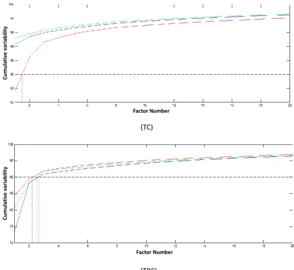
Figure 3.3 PCA scree plot. The normalised scree plots for individual components C, T, P, TC and TPC mixtures for three replicates are shown. Each of three replicate samples is plotted in three different colours. Only the first twenty principal components are presented. In each plot dashed lines show 90% cumulative variability, indicating the number of factors required to approximate at least 90% characteristics of the original samples. ... 47
Figure 3.4 Scores and loading plots produced using PCA for C1, C2 and C3 samples.
Score images are presented on the left showing the spatial information of each PC and loadings are presented on the right indicating the intensity of PCs. ... 49
Figure 3.5 Corresponding Score images at each significant peak from the original data for C1, C2 and C3 species samples. (A-C) are the total ion images of C1, C2 and C3 samples. The corresponding scores images at significant peaks are also shown. ... 51
Figure 3.6 Species C1 score image for peak at m/z = 191.02 ... 52
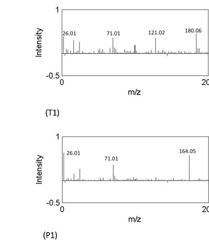
Figure 3.7 Scores and loading plots produced using PCA for T1 and P1 species samples.
Figure 3.8 Scores images and loading plots produced using PCA for TC1 species sample.
First PC and second PC are shown in the upper and lower row, respectively. ... 54
Figure 3.9 Score images and Loading plots produced using PCA for TPC1 mixture samples. ... 56
Figure 3.10 Sampled datasets from the original dataset. Sample size of 4096, 1024, 256, and 64 (shown as the black points in the images) have been randomly selected from the original dataset, from upper left to bottom right. ... 58
Figure 3.11Difference ratio between original dataset and different experiment dataset.
Errors between the results of original dataset and sampled dataset for PC1 (blue curve), PC2 (red curve) and PC3 (green curve) are given separately. ... 59
Figure 3.12 Loading plots produced using PCA for TPC1 sampled datasets. Three PCs are ordered in descending order according to the degree of importance. ... 61
Figure 3.13Scores images and loading plots produced using PCA with random sampling of a sample size of 4096 for TPC1 mixture. Score images are presented on the top while loadings for each of three PCs are shown below. ... 62
Figure 4.1 Three sets of loadings and scores images from NMF application for each pure component (T, C, and P) samples respectively. Scores images and loading plots are given for each species. ... 75
Figure 4.2Convergence of experiments with different factors and number of iteration.
This diagram shows the Frobenius norm errors between the original data X and the product of the factorisation matrices WH with respect to the changes of different factor numbers and number of iteration, which indicate the speed of convergence of NMF. ... 76
Figure 4.3 Scores images and loading plots from factorisation of TC1 mixture samples using NMF, two factors are utilised. ... 77
Figure 4.4 The Frobenius norm errors of experiments with different iteration numbers.
This diagram shows the convergence of the NMF algorithm with different iteration numbers for the mixture TC and TPC respectively. ... 78
Figure 4.5 Scores images and loading plots produced using NMF for TPC1 mixture samples. Three spectral factors are given on the bottom of each pannel. ... 80
Figure 4.6 Scores images and loading plots produced using sparsity constraint NMF for TPC1 mixture samples. Different regularising parameters were chosen for each experiment. ... 81
Figure 5.1 NMF model order selection using Chib’s method. The plots represent the marginal likelihood for individual component of the three pure chemical samples, T, P, and C. Only the models within 5 factors are presented. ... 91
Figure 5.2 NMF model order selection using Chib’s method. The plots represent the marginal likelihood for individual component of the two mixtures samples, TC and TPC. Only the models within 5 factors are presented. ... 92
Figure 5.3 Convergence rate of B-NMF algorithms for the TPC mixture The B-NMF algorithm converges fairly fast since the cost function is stabilised after only 50 iterations. ... 93
species samples. Scores images are on the left showing the spatial information of each factor while loading plots are on the right indicating the factors. ... 94
Figure 5.5 Scores images and loadings plots produced using B-NMF for T1, C1 and P1 species samples with additional factor numbers. Scores images are on the left showing the spatial information of each factor while loadings are on the right indicating the basis. ... 97
Figure 5.6 Scores images and loadings plots produced using B-NMF for TC1 mixed species samples with Models of 1, 2 and 3 factor numbers. Scores images are on the left showing the spatial information of each factor while loadings are on the right indicating the factors. ... 99
Figure 5.7 Scores and loadings images produced using B-NMF for TPC mixed species samples with Models of 2 and 3 factor numbers. Scores images are on the left showing the spatial information of each factor while loadings are on the right indicating the factors. ... 101
Figure 5.8 Spatial location for each species in TPC1 mixture sample. The three images implies the spatial location for each species in the mixture, T (m/z = 180.06), C (m/z = 191.02) and P (m/z = 164.06) are shown from left to right. ... 102
Figure 5.9 Scores images and loading plots produced using B-NMF combined random sampling method for TPC mixed species sample. Several sample number have been chosen with the range from 85% to 90% reduction of the raw data. Scores images are on the left showing the spatial information of each factor while loadings are on the right indicating the factors. ... 104
Figure 6.1 Example of a basis decomposition. A 128 pixels by 128 pixels ToF-SIMS image decomposed by a 4×4 grid of basis functions. The basis functions (shown by green curves) are scaled by the weight matrix, A. The centre of each basis function is shown by a yellow dot. The image is mapped onto -1 to 1 with arbitrary units. ... 116
Figure 6.2 Three sets of loading plots and scores images from ANLS application for each pure component (T, C, and P) samples respectively. Loadings are presented on the top of each panel indicating the intensity of spectral basis while score images are presented on the bottom showing the spatial information of each basis... 119
Figure 6.3 Three sets of loading plots and scores images using ANLS for TC mixture.
Loadings are presented on the top of each panel indicating the intensity of spectral basis while score images are presented on the bottom showing the spatial information of each basis. ... 120
Figure 6.4 Three sets of loading plots and scores images using ANLS for TPC mixture.
Loadings are presented on the top of each panel indicating the intensity of spectral basis while score images are presented on the bottom showing the spatial information of each basis. ... 121
Figure 6.5 loading plots and scores images using ANLS for single species T, P and C replicate samples with one basis. ... 123
Figure 6.6 Two sets of loading plots and scores images using ANLS for replicate TC mixture samples with two basis. ... 124
mixture samples. ... 125
Tables:
Table 2.1 Merging Algorithm ... 21Table 3.1 Significant peaks identified from PC loadings for C1, C2 and C3 pure species samples. The peak locations are displayed in an ascending order. ... 50
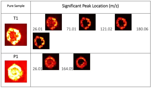
Table 3.2 Significant peaks identified from PC loadings produced using PCA for pure T1 and P1 samples. The locations are presented in an ascending order. Total ion images and corresponding score images are given alongside. ... 53
Table 3.3 Identified m/z values for peak assignment. All of the peaks can be used to identify specific individual chemical compounds while the numbers in red are the given ground truth for each chemicals. They can be used as references for the later identification of different species throughout this thesis. ... 53
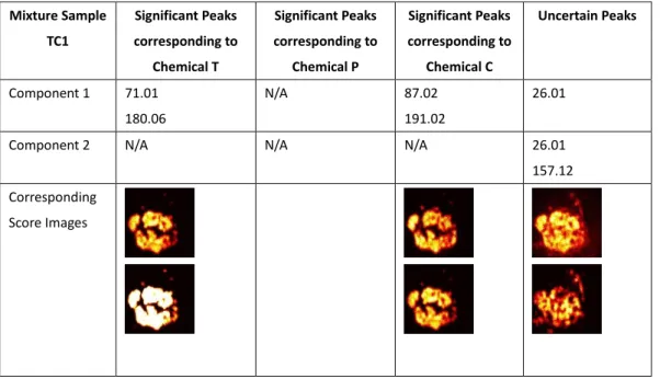
Table 3.4 Significant peaks identified from PC loadings produced using PCA for TC1 mixture samples. ... 55
Table 3.5 Significant peaks identified from PC loadings produced using PCA for TPC1 mixture species samples. The peak locations are displayed in an ascending order. . 57
Table 4.1 Alternating Least Squares Algorithm for NMF ... 71
Table 5.1 Gibbs Sampling Procedure ... 88
Table 5.2 B-NMF Algorithm... 90
Abbreviation List
ACLS Alternating Constrained Least Squares AHCLS Alternating Hoyer-Constrained Least Squares
ALS Alternating Least Squares
ANLS Alternating Non-negative Least Squares
B-NMF Non-negative Matrix Factorisation under Bayesian Framework
C Citric Acid
EFA Evolving Factor Analysis
EPSEM Equal Probability of Selection Method
ESI Electrospray Ionisation
ESS Error Sum of Squares
EVD Eigenvalue Decomposition
FC-NNLS Fast combinatorial Non-negativity constrained Least Squares
GC-MS Gas Chromatography Mass Spectrometry
HMDS Hexamethyldisilazane
ICA Independent Component Analysis
ITTFA Iterative Target Transformation Factor Analysis
LC-MS Liquid Chromatography Mass Spectrometry
MAF Maximum Autocorrelation Factor
MALDI Matrix-assisted Laser Desorption Ionisation
MCMC Markov Chain Monte-Carlo
MCR Multivariate Curve Resolution
MCR-ALS Multivariate Curve Resolution Alternating Least Squares
MLE Maximum Likelihood Estimation
MS Mass Spectrometry
MVA Multivariate analysis
NMF Non-negative Matrix Factorisation
NMR Nuclear Magnetic Resonance
P Phenylalanine
PCA Principal Components Analysis
PC Principal Component
SFA Sub-window Factor Analysis
SIMPLISMA Simple-to-use Self-modelling Mixture Analysis
SVD Singular Value Decomposition
T Tyrosine
ToF-SIMS Time-of-Flight Secondary Ions Mass Spectrometer
Chapter 1
Introduction
1.1
Background
Metabolomics is one of the most profound and significant milestones in the long history of life science research. Since it was developed in the mid-1990s, metabolomics has become a vital part of biological systems and has already penetrated into many important research subjects. While genomics and proteomics strive to explore the activities of life from the aspect of genes and proteins, many of the inter-cellular life activities is actually regulated by metabolites, such as cell signalling, energy transfer, as well as the inter-cellular communication. Metabolites can be considered as a reflection of the environment in the cell, which contains information about the nutritional state, the effects of drug treatment and environmental changes, and the impacts of other external factors (Clarke &
Haselden, 2008). Some researchers believe that, as compared with genomics and proteomics, metabolomics would play an increasingly important role in clinical practice (Schmidt, 2004). It can provide an in-depth examination of the actual impacts from gene expression with less information required.
The term “metabolic profiling” refers to the process of measuring the chemical reactions or dynamic responses of metabolites to external factors (Miura et al., 2009). This terminology was introduced by Horning et al. in the early 1970s when they studied the compounds in human biological samples, which was based on the idea initially developed by Williams et al. (1956) that human biological fluids might carry certain type of patterns or gene expression of genetically caused diseases. Nowadays, metabolic profiling has been widely approved by professionals and academic society, owing to its ability to examine the changes caused by external factors, understand the biological variation, detect genetic diseases in the early stage, and allow more tailored health solutions (Clarke & Haselden, 2008).
The main metabolic profiling tools are nuclear magnetic resonance (NMR) and mass spectrometry (MS) (Beckonert et al., 2007). NMR is a relatively insensitive tool which is particularly suitable for identification of structural information of metabolites (Ibáñez et al., 2013). By detecting the NMR spectra of a series of samples, the pathophysiological state of an organism can be determined with pattern recognition methods. It is also possible to identify the biomarkers in order to provide a predictable platform for the relevant research. By contrast, MS is typically combined with some separation techniques, such as liquid chromatography (LC-MS) and gas chromatography (GC-MS), in order to study specific chemicals or substances of interest (Clarke & Haselden, 2008).
In general, MS related technologies outperform NMR in the sense that it is capable of providing spectra with high sensitivity and resolution (Ibáñez et al., 2013). The most common MS include quadrupole, time-of-flight (ToF) analysers, magnetic sectors, Fourier transform, and quadrupole ion trap, among which ToF-SIMS
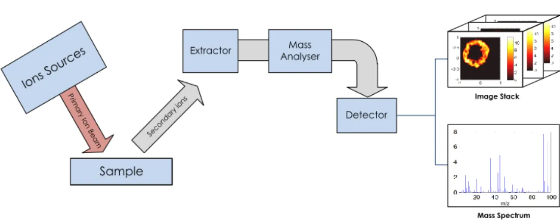
(time-of-flight secondary ions mass spectrometer) is one of the most powerful surface characterisation techniques that allows spectral analysis and direct chemical state imaging (Choi et al., 2003;Belu, Graham, & Castner, 2003). Similar to many other spectrometers, the main function of ToF-SIMS is to separate or resolve the ions formed in the ionisation source according to their mass-to-charge (m/z) ratios. The m denotes the mass number of the molecule since the molecular ion is equal to the molecular weight of the compound, while z refers to the charge number of the ion. Tof-SIMS is typically implemented along with some imaging mass spectrometer techniques, such as matrix-assisted laser desorption ionisation (MALDI) and electrospray ionisation (ESI) (Cotter, 2011). With the assistance of ToF-SIMS, researchers can obtain large amount of information about the biomolecules from the mass spectral features of the metabolites samples. The following chart shows the basic structure of a typical secondary ions mass spectrometer (Figure 1.1): Sample Prim ary Io n B eam Ions So urces Seco ndar y ion s Extractor Detector m/z Image Stack Mass Analyser Mass Spectrum
Figure 1.1 The basic structure of a secondary ions mass spectrometry. The sample is mass analysed using secondary ions mass spectrometer, static SIMS spectra from the surface of samples can be obtained by the end of the spectrometer process. The ions sources can be employed in three ways: surface ionisation, electron ionisation and liquid metal ionisation, with Bi+, Bi3+, Bi3++, Cs+ and C60+ ion sources commonly equipped (Dubey et al.,2011).
The flexibility of the ToF-SIMS technique and the high utility of data produced have generated strong interest in its application for biochemical characterisation (Belu, Graham, & Castner, 2003). While ToF-SIMS has been originally utilised in material
science, there is a growing research effort on the application in bioscience field, such as analysis of lipid, peptide, tumour spheroids and cancer cell samples (Vickerman & Briggs, 2001; Passarelli & Winograd, 2011; Kotze et al., 2013; Aoyagi et al., 2013).
1.2
Motivation and Purpose
ToF-SIMS is increasingly popular due to its in-situ ion separation methodology. It involves the free flight of the ionised molecules in a field-free drift tube. ToF-SIMS is widely utilised by analysts and researchers because of the following notable features (Belu, Graham, & Castner, 2003):
Fast parallel detection of all ions and high sensitivity
High mass range (theoretically unlimited)
High mass resolution > 10,000
High mass accuracy (1-10 ppm)
High transmission and spatial resolution
Ability to cover all elements, isotopes, as well as molecular species
While the advantages of ToF-SIMS are particularly attractive to metabolomics research and application, the output data can be substantially large due to the high spectral and spatial resolution (Graham, Wagner, & Castner, 2006). It is therefore very difficult to find relevant information or detect specific species, which makes data mining problematic (Sodhi, 2004).
The output data of ToF-SIMS can be represented as a combination of thousands of individual spectrum. One typical ToF-SIMS spectrum contains hundreds or thousands of different intensity peaks, depending on the order, structure, composition, and orientation of the surface species. It is not uncommon that many of the peaks within a given spectrum are somehow interrelated, since they are often derived from the same surface species. As a result, one of the challenges in
ToF-SIMS data analysis is to determine which peaks are interrelated and how they contribute to the chemical differences present on the surface. This is further complicated by the fact that ToF-SIMS dataset typically contains multiple spectra generated from multiple samples, which result in a large and complex data matrix to be analysed.
The large size of the output dataset can cause a number of problems for the interpretation of metabolites. When comparison between two features needs to be made, the high cost of computation caused by a large dataset would hamper the research process and incur considerable costs. Thus ToF-SIMS dataset is usually decomposed into different profiles containing distinct components, which also provide the possibility of template matching with stored templates in a database. Another serious concern for analysing large ToF-SIMS dataset is that it is extremely difficult to separate the original chemical compounds from fragmentation of species resulting in numerous number of peaks, especially when prior knowledge of the components is not available. Therefore, researchers always attempt to explore appropriate and efficient techniques that can be used to address the problems arising from ToF-SIMS data analysis (Tyler, Rayal, & Castner, 2007).
Since metabolic profiling appears to be a new area of application for ToF-SIMS, there are only a few algorithms currently available to handle the output data from metabolite samples. Thanks to prior development of dimensionality reduction and noise removal techniques, several multivariate analysis techniques have been suggested for large and multi-dimensional chemical spectral data processing, such as Principal Components Analysis (PCA), Maximum Autocorrelation Factors (MAF), and Multivariate Curve Resolution (MCR) (Tyler, 2006). However, none of them can efficiently extract information from a large dataset while produce a clear representation and interpretation in the context of metabolic profiling analysis. Therefore development of novel and innovative algorithms are undoubtedly needed to demonstrate the potential of ToF-SIMS for metabolic profiling analysis. In
this thesis, novel multivariate analysis techniques for processing ToF-SIMS data extracted from metabolite samples are derived and its application demonstrated.
1.3
Materials and Methods
The data set used throughout this thesis was obtained from the Department of Chemical and Biological Engineering, University of Sheffield. Three metabolites, tyrosine (T), phenylalanine (P) and citric acid (C) (all from Sigma Aldrich, UK) were used in the study. They are spotted on a dish as individual pure species and mixed species, resulting in a total of five separate experiments and each having three replicates. TC mixture contains T and C species in equimolar proportions and TPC mixture comprises T, P, and C species in equimolar proportions. These metabolites were spotted on hexamethyldisilazane (HMDS) (Sigma Aldrich, UK) coated silicon wafers (Compart Technology, UK), prepared as detailed by Salim, Wright, & Vaidyanathan (2012). The images consisted of 128 × 128 pixels. Each spectrum was calibrated using hydrocarbon fragment peaks. Spectral data up to m/z = 200 was considered for analysis although only the intensities for 100 m/z data points were provided for the image analysis for this work.
The given dataset with known chemical compounds provides us with a controlled environment in which to test the performance of any developed algorithm. The use of the known dataset also provides the ground truth and gives us the ability to interpret whether the results have a valid explanation. This is particularly important when using scale dependent methods such as PCA or MCR since the results obtained will be affected by the assumptions made when pre-processing the data. However, there is no knowledge of the exact spatial localisation of the different species, no quantitative measures exist to test for the complete validation of a given result. The development of the methods and their analysis was carried out using one dataset and tested with the two replicates in order to examine and validate the
results.
The underlying properties of the data that any algorithm needs to exploit result in the following requirements for the algorithms to be developed:
1. Dimensionality reduction – Removing redundant information 2. Feature extraction – Identification of discriminatory spectral peaks 3. Factorisation – Separation of spatial and spectral information
4. Sparsity analysis – Exploit redundancy in data (number of components) 5. Spatial correlation analysis – Exploiting spatial correlation
These requirements were the backbone for the development of the methodologies in this thesis.
1.4
Thesis Structure
The remainder of this thesis is organised as follows:
Firstly, a brief background and general working principle of the ToF-SIMS process will be detailed in Chapter 2. An outline of several multivariate analysis methodologies that have previously been suggested for ToF-SIMS data analysis are discussed and their contribution to ToF-SIMS data processing is reviewed.
Chapter 3 presents the implementation of a widely used method, the principal component analysis (PCA) to the ToF-SIMS dataset. This application is an unsupervised analysis procedure aimed at extracting features from large scale dataset while reducing the dimensionality. This implementation results are discussed and is shown to be promising in overcoming the complexity challenges presented by ToF-SIMS data.
Chapter 4 introduces a non-negativity constrained algorithm, namely non-negative matrix factorisation (NMF), which focuses on improving the interpretability of the
results. This exploits the fact that ToF-SIMS data are essentially non-negative quantities. Unlike the PCA and other multivariate analysis techniques, this algorithm is capable of providing physically meaningful results and facilitating data mining procedure.
The algorithm in Chapter 4 is extended in Chapter 5 by incorporating a Bayesian framework, and referred to as B-NMF. This method shows its capability in reducing the uncertainty and correlations that exist in the dataset. Moreover, it also provides an appropriate number of components indicative of the number of species in an unknown complex metabolic system.
A novel Alternating Non-negative Least Squares method (ANLS) is presented in Chapter 6. This technique is combined with MCR in order to take advantage of its ability to identify the chemical compounds or species of interest while taking the spatial correlation into account. It provides a simplified approximation of the data by implementing a dimensionality reduction method based on a basis function decomposition approach, significantly reducing the computational demand. This novel algorithm has high potential to be used as a effective tool in processing ToF-SIMS data extracted from metabolite samples.
The conclusions from the findings of the thesis are given in Chapter 7, where we will also discuss possible improvements that can be made to the analysis methods proposed here. It also includes suggestions for future research in metabolic profiling.
Chapter 2
Multivariate Statistical Analysis
Methods
2.1
Introduction
Perhaps no other instrument that is more indispensable than mass spectrometer to today’s science research. It has also become an essential tool in metabolic profiling analysis (Balmer et al., 2013). Because of the accuracy and high sensitivity provided, a ToF-SIMS can produce a high dimensional data cube, which provides detailed molecular information and high spatial resolution. However, due to the complexity of the species and the fragmentary nature of ToF-SIMS dataset, the resulting data is not always easy to interpret. This poses a serious threat to the usefulness and practical applications of mass spectrometer related techniques. Several multivariate
analysis methods have been previously used in addressing this problem. Currently the most popular method is principal component analysis (PCA) with singular value decomposition (SVD) approach, which is a basic as well as one of the earliest decomposition methods (Pearson, 1901; Hotelling, 1933). It identifies discriminatory features by finding the new projection with maximum variances between the components. Maximum autocorrelation factors (MAF) is an alternative to PCA based on maximising the autocorrelation between neighbouring pixels (Switzer & Green, 1984; Larsen, 2002). Another similar method is independent component analysis (ICA), it selects component from one unknown ‘blind’ mixture with a more rigorous assumption that the components are independent to each other (Linsker, 1992; Bell & Sejnowski, 1995). By contrast, multivariate curve resolution (MCR) is a feature extraction technique that is useful for providing the pure spectra of components in the system (Lawton & Sylvestre, 1971; de Juan & Tauler, 2006). Some other classical statistical methods, like clustering, can provide the benefit of grouping components with similar patterns into subsets.
This chapter will firstly provide a brief background of ToF-SIMS and description of its basic working principle. We will then explain the property a method should have to solve those problems by introducing the general data problem of ToF-SIMS. In addition, we will outline several well-known methodologies that have been extensively used in processing multi-dimensional data, including clustering, PCA, ICA, MAF, and MCR.
2.2
Background
A century has passed since the first prototype of mass spectrometer was originated by the winner of 1906 Nobel Prize in Physics, Sir Joseph John Thomson (Downard, 2012). This special analyser provides mass spectrum of an identical chemical sample, which is a plot of the ion signal as a function of the mass-to-charge ratio.
Mass spectrum can be considered as the fingerprint of the chemicals compounds. It is useful for determining the composition of the molecules, the distribution of chemical species, and chemical structures on the observed surface (Sodhi, 2004). Mass spectrometry can provide numerous possibilities for the analysis of complex systems, especially in the field of chemistry, biology, geology, military, environment and astronomy.
Currently, considerable research effort has concentrated on mass spectrometer and hence the inventions of different kinds of support machines. Different mass analysers vary in features, including the m/z range that can be covered, the mass accuracy, and the achievable resolution. An effective spectrometer will provide a detailed surface characterisation in order to not only identify the temporal and spatial patterns, but also verify the desired changes have been made. These factors require the ability to obtain the distribution, structure and chemical compounds of the surface species (Belu, Graham, & Castner, 2003).
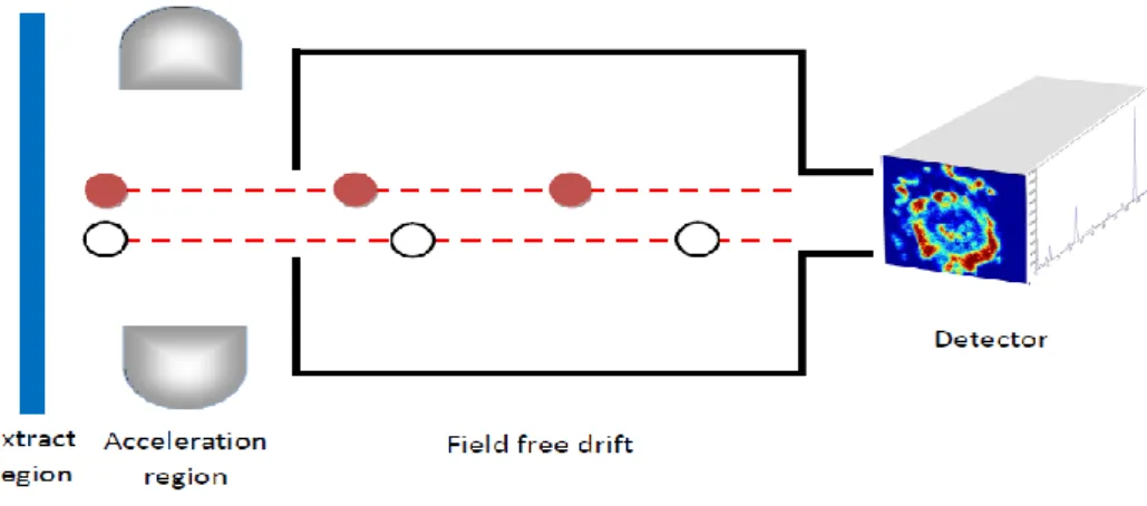
A ToF-SIMS determines the masses of secondary ions by recording their flight time (Choi et al., 2003). It utilises a pulsed ion beam to obtain secondary ions, which are then forced into the ToF analyser by a fixed high voltage (Sodhi, 2004). The extracted secondary ions are subsequently accelerated into the field-free drift tube, and a detector is placed at the finishing point of the flight path in order to monitor the pulses of these secondary ions. To ensure constant ion energy, ToF-SIMS typically incorporates a number of techniques to manage the differences in the initial condition and the energy dispersion of the extracted secondary ions. One ToF analyser working schematic is shown in Figure 2.1.
Figure 2.1 ToF-SIMS working procedure schematic diagram. Two secondary ions are accelerated to fly via the field free drift to reach the detector. The light (white) one approaches the detector earlier than the heavy (red) one.
Given the same amount of energy provided during this process, the only difference between secondary ions’ flight time is the velocity, which is primarily determined by their masses (Belu, Graham, & Castner, 2003). This relationship is shown as follows:
The velocity of secondary ions in a constant energy state can be simply expressed as:
velocity = √2×energymass (2.1) There is a positive relationship between flight-time and the mass of ion, as it can be demonstrated with a simple algebraic rearrangement:
Flight time =drift lengthvelocity = drift length × √2×energymass (2.2) Thus a set of flight times will give a set of mass values that can be plotted as mass spectrum.
A major strength of time-of-flight mass spectrometer is parallel detection of ions, which means that it is possible to capture all the secondary ions of different masses and generate a complete mass spectrum (Boxer, Kraft, & Weber, 2009). Whereas, many other mass spectrometers, such as quadrupole analyser and magnetic sector
analyser, are subject to a restricted mass range and lower mass transmission (Reed & Vickerman, 1993). In other words, the mass spectra produced by these mass spectrometers only represent the ions within a given mass range. Thus, parallel ion detection allows ToF-SIMS to handle secondary ions of high masses and have a relatively high sensitivity. Beside excellent sensitivity and high mass range, ToF-SIMS also benefits from high mass and spatial resolution (Belu, Graham, & Castner, 2003). This has made ToF-SIMS a promising instrument for biological analysis applications.
One typical ToF-SIMS mass spectrum may contain hundreds of peaks. The relative intensities of many of these peaks are interrelated since they come from the same surface species. In addition, even for the simplest single component samples, changes in the surface chemistry can affect the relative intensities of the peaks for a given sample system.
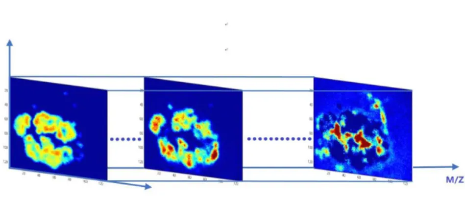
A typical ToF-SIMS dataset is illustrated in Figure 2.2 as a microscopic image cube of a sample surface along its mass spectrum (m/z). An image can be created for each mass with the loadings of the corresponding mass scores in every pixel. In our case, the replicate mixture dataset contains several 128 × 128 image stacks along the mass spectrum up to m/z = 100.
In the remainder of this chapter, we will outline several traditional multivariate techniques which are capable of identifying and extracting the useful information from large dataset, and hence reconstructing a data matrix with lower dimension.
2.3
Multivariate Analysis Techniques
The three-way array data in Figure 2.2 is made of mass spectra throughout the sample surface, in which multivariate analysis (MVA) methods are useful to provide insight to the identification of unknown number and types of the chemicals. This requires feature detection and extraction ability. Two types of defining and learning analysis methods are commonly used: supervised learning and unsupervised learning.
Supervised learning is probably the most straightforward analysis method that aims to seek for one satisfactory model with a set of given inputs and outputs. In our thesis, there is no prior information available, therefore an unsupervised learning would be more appropriate. In unsupervised learning, analysis typically involves detecting patterns and categorising objects purely based on the statistical characteristics.
While supervised learning model is utilised with sets of known inputs and outputs, no examples are given to the model in the unsupervised learning. Instead, patterns are derived directly from the given data, which is the case in our project. Moreover, it is possible to find the hidden structure from the unknown data using unsupervised learning.
Two popular method widely used in unsupervised learning are clustering and factorisation. Clustering is the grouping procedure which classifies similar components according to specific measurements. It is a main task of exploratory data mining as well as a common technique for statistical data analysis. By contrast,
factorisation is one “blind” feature identification technique offering dimensionality reduction benefit, it involves many different approaches, such as principle component analysis (PCA), independent component analysis (ICA), non-negative matrix factorisation (NMF), etc. All of these algorithms seek to extract and explain the key patterns of the data.
2.4
Clustering Analysis
Clustering is a statistical procedure for identifying object groups with similar patterns. It became well-known due to its application in psychology for personal trait classification (Cattell, 1943). The objective of clustering analysis is to split a set of objects into distinct groups (classes, clumps, and clusters) based on a chosen criterion (Jain, Murty, & Flynn, 1999).
The process of clustering is similar to classification, as they all deal with finding the relationship inside the dataset. However, a pre-training step for defining the groups’ characters is usually needed for a classifier, it would then learn from the different data group with the ability to classify. This process is a supervised learning as we mentioned previously. Whereas, clustering an unsupervised learning in which the grouping procedure is solely driven by the similarity within the data. It is therefore important to determine how to define the similarity.
Methodology
There are two classes of clustering method, one is called distance-based clustering which uses the distance between each objects as the similarity criterion; another clustering approach is called conceptual clustering which uses the concept in common to all objects as criterion (Jain, Murty, & Flynn, 1999; Michalski & Stepp, 1983). The latter one is much more complicated than the former kind, because the objects are organised according to certain ‘descriptive concept’, which is different
from the simple similarity measure.
Various mathematical methods are now widely implemented in the clustering algorithm, among which, Hierarchical method, Partitioning method, Density-based method, Grid-based method, Model-based method are five popular ones. The first two methods are based on the statistic distance of objects. Hierarchical clustering, for instance, is based on the union or the division of the dataset (Johnson, 1967). The procedure can be obtained in two ways: divisive and agglomerative, the principle can be shown as the graph below:
Figure 2.3 Hierarchical clustering procedure tree. Divisive clustering sets all the objects into one cluster at the beginning and splits them into different clusters step by step while agglomerative approach involves the reverse procedure.
Agglomerative procedure is based on the union between the two “nearest” clusters regarding to the distance, whereas, the divisive algorithm is based on the division of each cluster (Jain, Murty, & Flynn, 1999). Because divisive clustering is a global method, in order to gain a global view, it requires other algorithms besides itself, leading to larger amount of computation, which is not practical in many cases.
Distance measure
Distance is the most important factor in many clustering algorithms, as it is one widely approved way to define similarity.
For a mapping d: U × U →/R
It is called a distance function if, for any x, y ∈ U:d(x, y) ≥ 0; d(x, x) = 0;
d(x, y) = d(y, x). This distance function is also a metric if: d(x, y) = 0 then x = y; And,
d(x, y) ≤ d(x, z) + d(z, y) (2.3) The best known distance measurement between two points in a plane, which is the Euclidean metric defined by:
d2(x, y) = ‖x − y‖2 = √(x − y)T(x − y) (2.4) The Euclidean metric can be generalised in two ways. The first method is a popular measure called Minkowski metric, which is given by:
d2(x, y) = ‖x − y‖p = √(x − y)p (2.5) It should be noted that the Euclidean distance is a special case when p = 2, while the Manhattan distance is another special case when p = 1.
The second method of generalisation is obtained by defining:
dB(x, y) = ‖x − y‖B= √(x − y)TB(x − y) (2.6) This equation is related to the famous Mahalanobis distance, however this concept is beyond the scope of our experiment and the Euclidean distance is preferred.
Scaling normalisation
Before the clustering analysis is performed, the relative scaling should be firstly considered, actually, scaling should be considered before many other algorithms.
The importance of the scaling can be illustrated in the following charts:
Figure 2.4 illustration of scaling problem. Two kinds of different classification choices can be made due to the different scale measurements.
Figure 2.4 shows a simple example of scaling problem for a 2-dimensional case, in which the axes have the same magnitude but with different scaling, resulting in different visualising positions of the four points, as well as different clusters definitions. In order to solve the problem, normalisation is typically required.
In this thesis, we use a normalisation method described by:
x′ =1
s(x − x̅) (2.7) Where x′ is the normalised new variables, x̅ is the mean value of the elements in
x, and s is the standard deviation of the vector x. Agglomerative algorithm
Let nk = m, where nk is the number of clusters in different clustering level, and
m is the number of the objects, or cases need to cluster at the beginning. Therefore there are m clusters containing one object each.
The computation of the distance between clusters can be confusing since the
0 0.1 0.2 0.3 0.4 0.5 0.6 0.7 0.8 0.9 0 2
distance between different clusters is not the same as the difference between different objects. This can be demonstrated in the following ways (Jain, Murty, & Flynn, 1999):
1. Single linkage clustering: the distance between two clusters equals to the shortest distance between the elements of each cluster.
2. Complete linkage clustering: the distance between two clusters is the longest distance between the elements of each cluster.
3. Average/weighted average linkage clustering: the distance between two clusters is considered as the (weighted) average of the distances between every element of each cluster.
4. Centroid/weighted centroid linkage clustering: the distance between two clusters is the distance between the (weighted) centres of each cluster.
5. Ward linkage clustering: the distance is defined in terms of the error sum of squares, ESS.
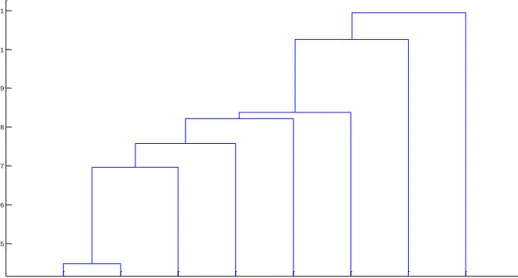
After the distance computation, a merging step would take place. At each iteration, the two clusters with the shortest distance are merged into one cluster. The iterative process would continue until the ideal cluster number is achieved. For example, if you want k clusters, simply cut off the procedure at the (k − 1)th iteration. The whole processing can be drawn as a linkage tree:
Figure 2.5Linkage tree of one hierarchical clustering. The 8 objects merge into one cluster at the end of the tree.
The horizontal axis in Figure 2.5 represents the labels of the clusters, the vertical axis stands for the distance level at every merging step. It can be seen in Figure 2.3, hierarchical clustering is considered as a bottom-up method and a divisive clustering would be considered as a top-down method, where one (or more) cluster is split into two clusters at every distance level.
Merging Algorithm
Merging steps
Arrange the m objects into a new order that results in a contiguous sequence. Choose any object to be the first one in the sequence s(1), the first gap (gap is the distance between clusters) is denoted as G(1) = ∞.
Select the nearest object as s(2), and the gap between s(1) and s(2) is
G(2) = d(s(1), s(2)).
From the rest objects, choose the one which is closest to one of s(1), s(2) as
s(3). Generalised, choose the s(k) as the closest element to any one of the ready-reordered sequence s(1), s(2), … , s(k − 1) and the gap is the distance
3 6 7 5 4 1 2 8 0.5 0.6 0.7 0.8 0.9 1 1.1
between the two elements, G(k).
Begin with the disjoint m clusters, and find the gap, which is the maximum of the all gaps (except G(1)), as Gmax, if the entire gaps before Gmaxare different,
then, merge the elements that has the minimum gap with the related element before into one clusters, there will be one cluster less.
Delete the rows and columns of the two merged objects, and add new row and column represent the new cluster s(m + 1), update the previous data sequence.
If all the objects are in one cluster, then the clustering should stop, otherwise, go back to the first step, loop again.
Table 2.1 Merging Algorithm
The computational demand of hierarchical clustering is considerably large though the calculation method is simple, especially the distance matrix. In addition, the algorithm only checks the local distribution at each merging step without checking the global distribution, therefore there is no way to change or revise what has been done. However, hierarchical clustering analysis remains a popular and easily understood method for distinguishing different groups within the data.
2.5
Principal Component Analysis (PCA)
Principal components analysis is claimed to be one of the most valuable contributions from applied linear algebra. It has been used widely in various fields due to its simplicity and outstanding applicability. The aim of PCA is to find the most meaningful basis to reconstruct a complex dataset based on a multi-dimensional orthogonal linear transformation (Hotelling, 1933). It assumes that the variables with the greatest variance are capable of explaining most part of the significant variations in the data (Abdi & Williams, 2010).
unreliable data mining and complicated computation. PCA intends to find the linear combination of the original variables (the principal components) by studying the covariance between the variables. It involves rotation of the covariance matrix into orthogonal factors where variables are no longer spatially correlated (Pearson, 1901).
Our ToF-SIMS dataset in this thesis are two spectral data points which are close to each other on the surface. Due to the inter-correlated nature of the dataset, there might be a large number of superfluous and pleonastic variables, which result in redundant computation and hamper the interpretation of the data. In this case, PCA may be used to remove the correlation in the data while retain the most representative information.
Methodology
The standard PCA algorithm is given by:
D = VX (2.8) Where D denotes scores matrix of principal components, V and X denote loadings matrix and the original matrix respectively. PCA can be performed using two approaches: eigenvalue decomposition (EVD) and singular vector decomposition (SVD).
1. EVD approach involves the calculation of eigenvalues and eigenvectors in which the eigenvalues refer to the degree of importance of the principal components and the eigenvectors are essentially the principal components. The raw data set is decomposed using EVD into several different ‘subsets’ with different importance indexes, and the first several important ‘subsets’ are selected as the principal components, which are believed to contain the most significant properties of the original dataset. One obvious pitfall of EVD approach is that it can only be applied to square matrix, which rarely occurs in reality. The formula of EVD is shown as follows:
Let X be a n × n matrix with N linearly independent eigenvectors,
qi(i = 1, , n) then we can decompose X as follows:
X = EΛE−1 (2.9) Where E is the eigen square matrix made of the X’s eigenvectors of qi and Λ is the diagonal matrix. The diagonal elements are the corresponding eigenvalues to the eigenvectors.
2. The general principle and formula of SVD are similar to EVD with a more generalised matrix size.
A m × n matrix X can be decomposed in the form of:
Xm×n= Um×m× Σm×n× Vn×nT (2.10)
Where U is an m × m orthogonal matrix, Σ is a m × n diagonal matrix with non-negative real numbers on the diagonal, and the n × n orthogonal matrix
VT denotes the transpose of V. This factorisation is called a singular value decomposition of X.
The relationship between singular value σ and eigenvalue λ can be illustrated by:
(WTX)v
i= λivi (2.11)
σi = √λi, ui=σ1
iXvi (2.12)
Where vi denotes the right singular vectors while ui is the left singular vectors. The entries of the diagonal matrix Σ are always listed in a descending order for the sake of calculation. In most cases, the first few singular values (principal components) may account for more than 90% of the entries in the data. Therefore the original dataset can be approximated using a far less number of variables, r, without losing the main information of the original dataset.
Xm×n≈ Um×rΣr×rVr×nT (2.13) One drawback of SVD can be illustrated in one O (N^3) calculation, which means that with the expansion of the matrix size, the computation will be complicated by three times, especially with a large number of r.
With the two approaches outlined above, PCA is able to obtain several largest eigenvalues or singular values, which are believed to contain the most significant characteristics of the data, and use them as the transformation matrix.
Ur×mT Xm×n ≈ Σr×rVr×nT (2.14) This formula can be generalised to one transformation with the rotation matrix T:
X̃r×n = Tr×mXm×n (2.15) PCA has been widely used as a dimensionality reduction technique in ToF-SIMS data analysis (Henderson, Fletcher, & Vickerman, 2009). However, Chang (1983) found that the large eigenvalues do not always represent the characteristics of the data; in particular, PCA might not be able to identify the linear combination if all the variables in the data that have the same variance.
2.6
Maximum Autocorrelation Factors (MAF)
Maximum autocorrelation factor (MAF) involves a transformation procedure which takes into consideration of the autocorrelation between neighbouring observations (Larsen, 2002). It was firstly proposed by Switzer and Green in 1984 as an alternative transformation method to PCA. In fact, MAF and PCA are mathematically similar if the covariance matrix is linearly related to the identity matrix (Switzer & Ingebritsen, 1986; Gallagher et al., 2014).
employs spatial autocorrelation as the criterion to decorrelate the data. The intuition has been widely accepted due to its sound assumption that noise tends to have a smaller spatial autocorrelation relative to significant components (Storvik, 1993). If noise components in the dataset have larger variance relative to the interesting components, PCA would lead to poor and unreliable representation, as it is unable to recognise whether the linear combination is attributed to the interesting components or noise (Keenan & Smentkowski, 2011). This means that MAF would outperform PCA when the interesting components have lower variance and higher autocorrelation than noise, vice versa (Larsen, 2002).
Methodology
MAF was developed on the basis of PCA. In order to account for autocorrelation between neighbouring observations, MAF employs a shifted matrix that is found by taking the difference between the original data matrix and a spatially shifted duplicate of itself (Tyler, Rayal, & Castner, 2007). The original dataset X can be decomposed by regular PCA method in Equation (2.3), where the matrix V is obtained by an eigenvector rotation of the MAF factor. In order to differentiate from PCA, the MAF transformation can be described by the following linear combinations:
S = ATX (2.16) Where the MAF factor A is obtained by
A = U2TΛ−12U
1 (2.17)
U1 denotes the eigenvectors while Λ denotes the eigenvalues of the matrix B, where B is the covariance matrix of the original dataset W, which can be specified by the equation below:
U1BU1T= Λ (2.18)
from the equation below:
U2X( )U2T= U
2(12([ΓW( )]T+ [ΓY( )]))U2T (2.19)
In this equation, ΓY is the spatial correlation, which is defined by Equation (2.20):
Γ( ) = Cov{Xk, Xk+ } (2.20) With the property given by:
ΓT( ) = Γ(− ) (2.21) Where k denotes the spatial position while is one spatial movement. The matrix derived via the MAF method transforms the variance-covariance matrix to the identity matrix and the shifted matrix for spatial shift of to a diagonal matrix. MAF produces uncorrelated variables with largest autocorrelations using joint diagonalisation of asymmetric covariance matrices.
2.7
Independent Components Analysis (ICA)
Independent Component Analysis (ICA) is also a widely applied tool for identifying components from mixtures and it has been presented in some particular spectral data analyses for the use of identifying the unknown components in the mixture as well as in estimating their concentrations without prior knowledge (Chen & Wang, 2000; Bayliss et al., 1998). ICA was firstly introduced by Herault and Jutten (1986) to address so called “blind source separation” problem based on the assumption that signals originated from different sources in a mixture are mutually independent in distribution (Comon, 1994). ICA is generally considered as an extension of PCA since it also transforms the data into uncorrelated factors. However, ICA employs a more rigorous criterion since statistical independence always leads to uncorrelation, while the converse does not necessarily hold (Hyvärinen & Oja, 2000). In addition, there is no order associated with the components extracted by ICA, whereas PCA
assumes that the first principal component has the largest explanatory power to the variation of the data (Langlois, Chartier, & Gosselin, 2010).
There are two major approaches for ICA algorithms, arising from different interpretation of the statistical independence (Haykin, 2009). InfoMax and Maximum Likelihood estimation are algorithms for ICA developed on the basis of information theory which minimises the Shannon mutual information of pairs of variables (Amari, Cichocki, & Yang, 1996; Bell & Sejnowski, 1995; Pham, Garrat, & Jutten, 1992). By contrast, FastICA is an approach based on the intuition that mutually independent distribution can be properly measured by the deviation from normal distribution (non-Gaussianity) (Hyvärinen & Oja, 2000). Therefore, a fundamental limitation of ICA is that the independent components must be non-Gaussian for ICA to be applicable.
Methodology
ICA transform seeks linear combinations that minimise the statistical independence between variables. InfoMax is the approach rooted in the minimisation of mutual information, which utilises entropy as a primary measure of the uncertainty.
InfoMax
Entropy can be considered as the degree of information that the observations of variables provide. Larger entropy is typically related to more random and unpredictable variables (Hyvärinen & Oja, 2000). Conversely, lower entropy means that we have more information about a given system. Entropy can be considered as a measure of non-Gaussianity since a Gaussian variable typically has the greatest entropy among all variables for a given variance. This means that Guassian variables have more “random” distributions. For a discrete random variable X, entropy H is defined as:
H (X) = − ∑ P(x)logP(x)𝑥 (2.22)
H (X, Y) = − ∑𝑥,𝑦P(x, y)logP(x, y) (2.24) Where P(x) is the probability that X is in the state x. Differential entropy is the case when the ordinary concept of entropy is generalised for continuous random variables. The differential entropy H of a random variable x with density f (x) can be described by:
H(x) = − ∫ f (x) log f (x)dx (2.25) The mutual information I between m (scalar) random variables, xi, i =
1. . . m can be defined as follows:
I(x1, x2, . . . , x𝑚) = ∑mi=1H(x𝑖) − H(x) (2.26) The mutual information can be interpreted as the Kullback-Leibler divergence between the joint density f (x) of random variables (Amari, Cichocki, & Yang, 1996). Therefore, mutual information is a proper measure of independence between random variables as it is non-negative in nature and equal to zero when the variables are statistically independent. By minimising the mutual information, we are able to identify the most statistically independent components. The methods based on mutual information minimisation are preferable in a changing environment (Langlois, Chartier, & Gosselin, 2010).
FastICA
Another approach to measure statistical independence also involves the concept of non-Gaussianity, where negentropy is used a quantitative measure of non-Gaussianity of random variables. Negentropy is a measure of the deviation from normality, which indicates the degree of statistical independence of variables. Negentropy is defined by:
J(x) = H(xGaussian) − H(x) (2.27) Where xGaussian is a Gaussian random variable with the same covariance matrix as
that of a non-Gaussian variable, x, and H(x) denotes the entropy. Similar to the concept of entropy, negentropy is always positive, but equal to zero only when the variable has a Gaussian distribution.
However, the computation of negentropy is complicated and approximation approaches are used. One effective approximation approach is called FastICA, which can be described by:
N(V) = E(∅(V)) − E(∅(U))2 (2.28) Where V is a non-Gaussian random variable, U is a Gaussian random variable and
∅(∙) denotes a non-quadratic function. A pre-processing process is required so that all variables are standardised. FastICA offers a computationally inexpensive way to extract independent components with non-Guassian or sub-Guassian distribution (Hyvärinen & Oja, 2000).
2.8
Multivariate Curve Resolution (MCR)
One typical criticism of PCA and other traditional algorithms is that the components extracted are essentially mathematical factors, which may or may not result in meaningful interpretation (Lachenmeier & Kessler, 2008). By contrast, Multivariate Curve Resolution (MCR) is a methodology that not only provides statistically significant results, but also offers practical importance to ToF-SIMS data analysis, especially for chemical and biological data (Wentzell et al., 2006;de Juan, Jaumot, & Tauler, 2014). It is capable of extracting the single properties of the chemical compounds of mixtures (the pure component spectra) and the concentration profiles with incomplete or even no knowledge of the components (de Juan & Tauler, 2006). This means that MCR can be used to process complex dataset or identify unknown chemical compounds.
approaches have gained great popularity due to the ability to process multiset data structures and incorporate known information into the iterative process as constraints (de Juan, Jaumot, & Tauler, 2014). One of the most commonly used iterative MCR algorithms is MCR-ALS which uses alternating least squares (ALS) to solve the optimisation problem at each iteration. We will provide more detailed description of one novel MCR-ALS in Chapter 4.
Although the advantage of MCR is particularly attractive to biological applications, it might produce multiple solutions for the dataset due to intensity and rotational ambiguity (de Juan, Jaumot, & Tauler, 2014). Intensity ambiguity is derived from the indeterminate magnitude of the concentration profiles and pure spectra, leading to different interpretation of identical statistical results (Wise & Kowalski, 1995). However, it is normally easy to be detected and can be mitigated by normalising the concentration profiles or spectra produced, or incorporating known information into the approximation (Tauler, Kowalski, & Fleming, 1993; de Juan, Jaumot, & Tauler, 2014). Analysts are generally more concerned about rotational ambiguity, which is resulted from multiplying or dividing the components by a rotated matrix. Rotational ambiguity can be suppressed by incorporating constraints into the algorithm (Lachenmeier & Kessler, 2008). Common constraints include non-negativity, unimodality, closure, and stoichiometry, among which non-negativity constraint has been used most widely to offer realistic and meaningful results (Tyler, 2006).
Methodology
MCR was initially devised as a tool to study a single second-order data matrix that follows a bilinear structure. It involves a transformation procedure that decomposes the original data matrix into the product of two matrices where each matrix corresponds to an order of the original matrix (Tauler, Kowalski, & Fleming, 1993). The application of MCR has now been extended to multi-dimensional data analysis and more complex systems. However, this requires that the original dataset can be