c
MODEL SELECTION FOR CORRELATED DATA AND MOMENT SELECTION FROM HIGH-DIMENSIONAL MOMENT CONDITIONS
BY
HYUN KEUN CHO
DISSERTATION
Submitted in partial fulfillment of the requirements for the degree of Doctor of Philosophy in Statistics
in the Graduate College of the
University of Illinois at Urbana-Champaign, 2013
Urbana, Illinois
Doctoral Committee:
Professor Annie Qu, Chair Professor Jeffrey Douglas Professor Xiaofeng Shao Professor Douglas Simpson
Abstract
High-dimensional correlated data arise frequently in many studies. My primary research interests lie broadly in statistical methodology for correlated data such as longitudinal data and panel data. In this thesis, we address two important but challenging issues: model selection for correlated data with diverging number of parameters and consistent moment selection from high-dimensional moment conditions.
Longitudinal data arise frequently in biomedical and genomic research where repeated measure-ments within subjects are correlated. It is important to select relevant covariates when the dimen-sion of the parameters diverges as the sample size increases. We propose the penalized quadratic inference function to perform model selection and estimation simultaneously in the framework of a diverging number of regression parameters. The penalized quadratic inference function can easily take correlation information from clustered data into account, yet it does not require specifying the likelihood function. This is advantageous compared to existing model selection methods for discrete data with large cluster size. In addition, the proposed approach enjoys the oracle property; it is able to identify non-zero components consistently with probability tending to 1, and any finite linear combination of the estimated non-zero components has an asymptotic normal distribution. We propose an efficient algorithm by selecting an effective tuning parameter to solve the penalized quadratic inference function. Monte Carlo simulation studies have the proposed method selecting the correct model with a high frequency and estimating covariate effects accurately even when the dimension of parameters is high. We illustrate the proposed approach by analyzing periodontal disease data.
The generalized method of moments (GMM) approach combines moment conditions optimally to obtain efficient estimation without specifying the full likelihood function. However, the GMM estimator could be infeasible when the number of moment conditions exceeds the sample size. This
research intends to address issues arising from the motivating problem where the dimension of esti-mating equations or moment conditions far exceeds the sample size, such as in selecting informative correlation structure or modeling for dynamic panel data. We propose a Bayesian information type of criterion to select the optimal number of linear combinations of moment conditions. In theory, we show that the proposed criterion leads to consistent selection of the number of principal com-ponents for the weighting matrix in the GMM. Monte Carlo studies indicate that the proposed method outperforms existing methods in the sense of reducing bias and improving the efficiency of estimation. We also illustrate a real data example for moment selection using dynamic panel data models.
I dedicate this dissertation to my parents.
Acknowledgments
Foremost, I would like to express my sincere gratitude to my advisor Dr. Annie Qu for her continuous support of my Ph.D. study and research, for her patience, motivation, enthusiasm, and immense knowledge. Her guidance helped me throughout my period of research and thesis writing. I could not have imagined having a better advisor and mentor for my Ph.D. study.
A special thanks to my thesis committee: Dr. Jeffrey Douglas, Dr. Xiaofeng Shao, and Dr. Douglas Simpson for providing valuable feedback and counsel during particularly difficult personal times that threatened to halt my entire research. Their encouraging words helped me work through all the distractions and noise. In addition to my advisor and committee, I would like to acknowledge my collaborators, Dr. Peng Wang and Dr. Jianhui Zhou for useful discussions about estimation procedures for longitudinal data, permission to use simulation code in my thesis as well as valuable and pleasant collaborative experiences.
Many thanks are given to my fellow students at the Department of Statistics. Particularly, I would like to thank Yeonjoo Park, Peibei Shi, Xinxin Shu, Samuel Ye, and Xianyang Zhang for their support, encouragement and friendship. And to the wonderful staff, Melissa Banks, you have always gone far beyond your job description to help us as graduate students. You are always available to take care of my myriad of any issues. Your efforts and time have been greatly appreciated.
Finally and most importantly, I want to thank my family for their constant support and prayers throughout my life but particulary during my years of study and research. Their unconditional love, encouragement, and dedication carried me on through difficult times.
Table of Contents
Chapter 1 Introduction . . . 1
Chapter 2 Model Selection for Correlated Data with Diverging Number of Pa-rameters . . . 3
2.1 Introduction . . . 3
2.2 Estimation Procedures for Longitudinal Data . . . 5
2.3 A New Estimation Method and Theory . . . 8
2.4 Implementation . . . 11
2.4.1 Local Quadratic Approximation . . . 11
2.4.2 Linear Approximation Method . . . 12
2.4.3 Tuning Parameter Selector . . . 13
2.4.4 Unbalanced Data Implementation . . . 14
2.5 Numerical Studies . . . 15
2.5.1 Correlated Binary Response . . . 15
2.5.2 Periodontal Disease Data Example . . . 17
2.6 Discussion . . . 19
2.7 Proofs of Theorems and Lemmas . . . 20
Chapter 3 Consistent Moment Selection from High-Dimensional Moment Con-ditions . . . 31
3.1 Introduction . . . 31
3.2 Dynamic Panel Data Models and Quadratic Inference Function . . . 34
3.2.1 Simple Dynamic Panel Models . . . 34
3.2.2 Dynamic Panel Data Models with Exogenous Variables . . . 36
3.2.3 Quadratic Inference Function . . . 37
3.3 A New Moment Selection Method and Theory . . . 39
3.4 Numerical Studies . . . 42
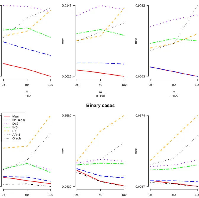
3.4.1 Correlated Continuous Response . . . 42
3.4.2 Correlated Binary Response . . . 44
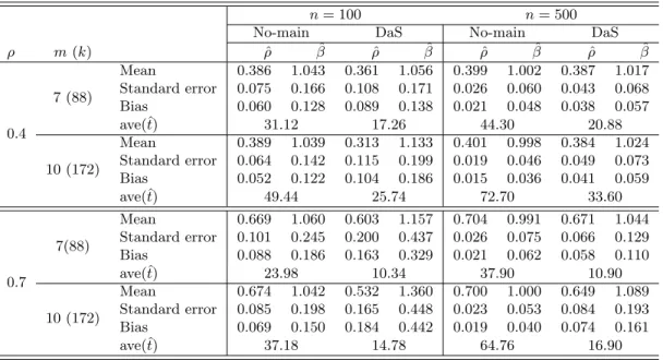
3.4.3 Dynamic Panel Data Models . . . 45
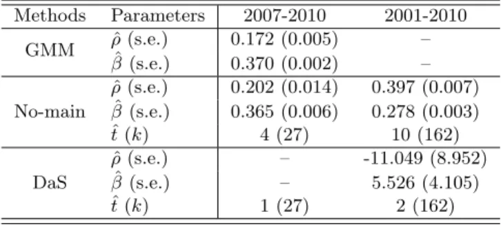
3.4.4 Fortune 500 Data Example . . . 46
3.5 Discussion . . . 47
3.6 Proofs of Theorem and Lemma . . . 48
Chapter 1
Introduction
Correlated data arise frequently in many studies where repeated measurements are taken from the same subject over time. Variable selection is fundamental to extracting important relevant predictors from large data sets, as inclusion of high-dimensional redundant variables can hinder efficient estimation and inference for the non-zero coefficients. In the longitudinal data framework, however, the research on variable selections is still limited when the dimension of parameters diverges.
In Chapter 2, we propose a penalized quadratic inference function (QIF) approach for model selection in the longitudinal data setting. We show that even when the number of parameters diverges as the sample size increases, the penalized QIF utilizing the smoothly clipped absolute deviation (SCAD) penalty function possesses desirable features of the SCAD such as sparsity, unbiasedness and continuity. The penalized QIF also enjoys the oracle property. That is, the proposed model selection is able to identify non-zero components correctly with probability tending to 1, and any valid linear combination of the estimated non-zero components follows the asymptotic normal distribution.
One of the unique advantages of the penalized QIF approach for correlated data is that the correlation within subjects can be easily taken into account as the working correlation can be ap-proximated by a linear combination of known basis matrices. In addition, the nuisance parameters associated with the working correlation are not required to be estimated as the minimization of the penalized QIF does not involve the nuisance parameters. This is especially advantageous when the dimension of estimated parameters is high, as reducing nuisance parameter estimation improves estimation efficiency and model selection performance significantly.
Another important advantage of our approach is in tuning parameter selection. The selection of the tuning parameter plays an important role in order to achieve optimal performance in model
selection. We provide an effective tuning parameter selection procedure based on the Bayesian information quadratic inference function criterion, and show that the proposed tuning parameter selector leads to consistent model selection and estimation for regression parameters.
In Chapter 3, we are motivated by the problem where the dimension of estimating equations or moment conditions far exceeds the sample size. For example, for correlated data, the dimension of moment conditions depends on the number of basis matrices associated with the inverse of the correlation matrix, and can be larger than the sample size. For dynamic panel data example, a large dimension of valid moment conditions can be generated based on the first-order moments.
The generalized method of moments (GMM, Hansen, 1982) is widely applicable when the likelihood function is difficult to specify, while moment conditions are easy to formulate. The GMM is powerful as it optimally combines valid moment conditions, and so is able to achieve estimation efficiency. However, the GMM could perform poorly if there are too many moment conditions relative to the sample size, due to limitation in finite samples.
To solve this problem, we examine the key element of the GMM: the optimal weighting matrix which is the inverse of the sample covariance matrix of moment conditions. In fact, the sample covariance matrix could be problematic when the dimension of the matrix is large due to the following two reasons: i) the sample covariance matrix is not of full rank if the dimension of moment conditions exceeds the sample size; ii) even if the sample covariance matrix is invertible, the estimation of its inverse could be biased with high variation when the number of moment conditions is close to the sample size. The singularity problem of the sample covariance matrix makes the GMM estimator infeasible or unstable.
We propose a new objective function based on a Bayesian information type of criterion which selects an optimal number of linear combinations of the moment conditions. This allows one to reduce the dimensionality of available moment conditions while retaining most of the important information from data. In theory, we show that the proposed criterion can select an optimal number of principal components consistently without loss of efficiency, when both the number of moment conditions and the sample size go to infinity. The proposed criterion can be applied to estimate the inverse of the covariance matrix in high-dimensional data settings, in addition to solving moment selection problems arising from dynamic panel data.
Chapter 2
Model Selection for Correlated Data
with Diverging Number of
Parameters
2.1
Introduction
Longitudinal data arise frequently in biomedical and health studies where repeated measurements are taken from the same subject. The correlated nature of longitudinal data makes it difficult to specify the full likelihood function when responses are non-normal. Liang and Zeger (1986) developed the generalized estimating equation (GEE) for correlated data, which only requires the first two moments, and a working correlation matrix involving a small number of nuisance param-eters. Although the GEE yields a consistent estimator even if the working correlation structure is misspecified, the estimator can be inefficient under the misspecified correlation structure. Qu, Lindsay, and Li (2000) proposed the quadratic inference function (QIF) to improve the efficiency of the GEE when the working correlation is misspecified, in addition to providing an inference function for model diagnostic tests and goodness-of-fit tests.
Variable selection is fundamental in extracting important predictors when the covariates are high-dimensional. Including high-dimensional redundant variables can hinder efficient estimation and distort inference for the non-zero coefficients for high-dimensional data. In the longitudinal data framework, several variable selection methods for marginal models have been developed. Pan (2001) proposed an extension of the Akaike information criterion (Akaike, 1973) by applying the quasilikelihood to the GEE, assuming independent working correlation. Cantoni, Flemming, and Ronchetti (2005) proposed a generalized version of Mallows’ Cp (Mallows, 1973) by minimizing the prediction error. However, the asymptotic properties of these model selection procedures have not been well studied. Wang and Qu (2009) developed a Bayesian information type of criterion (Schwarz, 1978) based on the quadratic inference function to incorporate correlation information. These approaches are the best sub-set selection approaches and have been shown to be consistent
for model selection. However, theL0-based penalty can be computationally intensive and unstable
when the dimension of covariates is high. Fu (2003) applied the bridge penalty model to the GEE and Xu et al. (2010) introduced the adaptive LASSO (Zou, 2006) for the GEE setting. Dziak (2006) and Dziak, Li, and Qu (2009) discussed the SCAD penalty for GEE and QIF model selection for longitudinal data. These methods are able to perform model selection and parameter estimation simultaneously. However, most of the theory and implementation is restricted to a fixed dimension of parameters.
Despite the importance of model selection in high-dimensional settings (Fan and Li, 2006; Fan and Lv, 2010), model selection for longitudinal discrete data is not well studied when the dimension of parameters diverges. This is probably due to the challenge of specifying the likelihood function for correlated discrete data. Wang, Zhou, and Qu (2012) developed the penalized generalized estimating equation (PGEE) for model selection when the number of parameters diverges, and this is based on the penalized estimating equation approach by Johnson, Lin, and Zeng (2008) in the framework of a diverging number of parameters by Wang (2011). However, in our simulation studies, we show that the penalized GEE tends to overfit the model regardless of whether the working correlation is correctly specified or not.
We propose the penalized quadratic inference function (PQIF) approach for model selection in the longitudinal data setting. We show that, even when the number of parameters diverges as the sample size increases, the penalized QIF utilizing the smoothly clipped absolute deviation (SCAD) penalty function (Fan and Li, 2001; Fan and Peng, 2004) possesses such desirable features of the SCAD as sparsity, unbiasedness, and continuity. The penalized QIF also enjoys the oracle prop-erty. That is, the proposed model selection is able to identify non-zero components correctly with probability tending to 1, and any valid linear combination of the estimated non-zero components is the asymptotically normal.
One of the unique advantages of the penalized QIF approach for correlated data is that the correlation within subjects can be easily taken into account, as the working correlation can be approximated by a linear combination of known basis matrices. In addition, the nuisance parame-ters associated with the working correlation are not required to be estimated, as the minimization of the penalized QIF does not involve the nuisance parameters. This is especially advantageous
when the dimension of estimated parameters is high, as reducing nuisance parameter estimation improves estimation efficiency and model selection performance significantly. Consequently, the penalized QIF outperforms the penalized GEE approach under any working correlation structure in our simulation studies. Furthermore, the penalized QIF only requires specifying the first two moments instead of the full likelihood function, and this is especially advantageous for discrete correlated data.
Another important advantage of our approach is in tuning parameter selection. The selection of the tuning parameter plays an important role in achieving desirable performance in model se-lection. We provide a more effective tuning parameter selection procedure based on the Bayesian information quadratic inference function criterion (BIQIF), and show that the proposed tuning pa-rameter selector leads to consistent model selection and estimation for regression papa-rameters. This is in contrast to the penalized GEE, which relies on cross-validation for tuning parameter selection. Our simulation studies for binary longitudinal data indicate that the penalized QIF is able to select the correct model with a higher frequency and provide a more efficient estimator, compared to the penalized GEE approach, when the dimensions of covariates and non-zero parameters increase as the sample size increases.
The rest of Chapter 2 is organized as follows. Section 2.2 briefly describes the quadratic in-ference function for longitudinal data. Section 2.3 introduces the penalized quadratic inin-ference function and provides the asymptotic properties for variable selection when the number of param-eters diverges. Section 2.4 presents two algorithms to implement the penalized QIF approach and a tuning parameter selector. Section 2.5 reports on simulation studies for binary responses and provides a data example from a periodontal disease study. Section 2.6 provides concluding remarks and discussion. All necessary lemmas and theoretical proofs are in Section 2.7.
2.2
Estimation Procedures for Longitudinal Data
Suppose the response variable for theith subject is measuredmi times,yi = (yi1, . . . , yimi)
T, where yi’s are independent identically distributed,i= 1, . . . , n,nis the sample size andmi is the cluster size. The corresponding covariate Xi = (Xi1, . . . , Ximi)
T is mi ×pn-dimensional matrix for the ith subject. In the generalized linear model framework, the marginal mean of yij is specified as
µij = E(yij|Xij) = µ(XijTβn), where µ(·) is the inverse link function and βn is a pn-dimensional parameter vector in the parameter space Ωpn ∈R
pn,pndiverging as the sample size increases. Since
the full likelihood function for correlated non-Gaussian data is rather difficult to specify when the cluster size is large, Liang and Zeger (1986) developed the generalized estimating equation (GEE) to obtain theβn estimator by solving the equations
Wn(βn) = n X i=1 ˙ µTi (βn)Vi−1(βn)(yi−µi(βn)) = 0, (2.1)
where ˙µi = (∂µi/∂βn) is a mi×pn matrix, and Vi = A
1/2
i RA
1/2
i , with Ai the diagonal marginal variance matrix of yi and R the working correlation matrix that involves a small number of cor-relation parameters. Although the GEE estimator is consistent and asymptotically normal even if the working correlation matrix is misspecified, the GEE estimator is not efficient under the misspecification of the working correlation.
To improve efficiency, Qu, Lindsay, and Li (2000) proposed the quadratic inference function for longitudinal data. They assume that the inverse of the working correlation can be approximated by a linear combination of several basis matrices, that is,
R−1 ≈
k X j=0
ajMj, (2.2)
where M0 is the identity matrix, M1, . . . , Mk are basis matrices with 0 and 1 components and a0, . . . , ak are unknown coefficients. For example, if R corresponds to an exchangeable structure, thenR−1=a0M0+a1M1,wherea0 anda1 are constants associated with the exchangeable
corre-lation parameter and the cluster size, andM1 is a symmetric matrix with 0 on the diagonal and 1
elsewhere. If R has AR-1 structure, then R−1 =a
0M0+a1M1+a2M2,where a0, a1, and a2 are
constants associated with the AR-1 correlation parameter,M1 is a symmetric matrix with 1 on the
sub-diagonal entries and 0 elsewhere, and M2 is a symmetric matrix with 1 on entries (1,1) and
(mi, mi). If there is no prior knowledge on the correlation structure, then a set of basis matrices containing 1 for (i, j) and (j, i) entries and 0 elsewhere can be used as a linear representation for R−1.
im-prove the efficiency of the regression parameter estimators. Zhou and Qu (2012) provide a model selection approach for selecting informative basis matrices that approximate the inverse of the true correlation structure. Their key idea is to approximate the empirical estimator of the correlation matrix by a linear combination of candidate basis matrices representing common correlation struc-tures as well as mixstruc-tures of several correlation strucstruc-tures. They minimize the Euclidean distance between the estimating functions based on the empirical correlation matrix and candidate basis matrices, and penalize models involving too many matrices.
By replacing the inverse of the working correlation matrix with (2.2), the GEE in (2.1) can be approximated as a linear combination of the elements in the following extended score vector:
¯ gn(βn) = 1 n n X i=1 gi(βn)≈ 1 n Pn i=1( ˙µi)TAi−1(yi−µi) Pn i=1( ˙µi)TA −1/2 i M1A −1/2 i (yi−µi) .. . Pn i=1( ˙µi)TA −1/2 i MkA −1/2 i (yi−µi) . (2.3)
Since it is impossible to set each equation in (2.3) to zero simultaneously in solving for βn, as the dimension of the estimating equations exceeds the dimension of parameters, Qu, Lindsay, and Li (2000) applied the generalized method of moments (Hansen, 1982) to obtain an estimator ofβn by minimizing the quadratic inference function (QIF)
Qn(βn) =ng¯n(βn)TC¯n−1(βn)¯gn(βn),
where ¯Cn(βn) = 1nPn
i=1gi(βn)giT(βn) is the sample covariance matrix of gi. Note that this mini-mization does not involve estimating the nuisance parametersa0, . . . , akassociated with the linear weights in (2.2). The quadratic inference function plays an inferential role similar to minus twice the log-likelihood function, and it possesses the same chi-squared asymptotic properties as in the likelihood ratio test. The QIF estimator is optimal in the sense that the asymptotic variance matrix of the estimator of βn reaches the minimum among estimators solved by the same linear class of the estimating equations given in (2.3).
2.3
A New Estimation Method and Theory
For correlated discrete data, existing approaches for model selection are rather limited due to the difficulty of specifying the full likelihood function. We propose a new variable selection approach based on the penalized quadratic inference function that can incorporate correlation information from clusters. The proposed procedure can estimate parameters and select important variables simultaneously in the framework of a diverging number of covariates. Even when the dimension of parameters diverges as the sample size increases, the proposed model selection contains the sparsity property and shrinks the estimators of the non-signal components to zero. In addition, the non-zero components are selected correctly with probability tending to 1. We also show that the estimators of the non-zero components are consistent at the convergence rate of pn/pn, and follow the normal distribution asymptotically.
Without loss of generality, the cluster sizes are taken to be equal,mi=m, although the cluster size is unbalanced in our data example. Since the response variables are not necessarily continuous, we replace the typical least square function by the quadratic inference function since it is analogous to minus twice the log-likelihood. We define it as
Sn(βn) =Qn(βn) +n pn
X j=1
Pλn(|βnj|). (2.4)
Among several penalty functions Pλn(·), we choose the non-convex SCAD penalty function
corre-sponding to Pλn(|βnj|) = λn|βnj|I(0≤ |βnj|< λn) + aλn(|βnj|−λn)−(|βnj|2−λ2n)/2 (a−1) +λ 2 n I(λn≤ |βnj|< aλn) + (a−1)λ2 n 2 +λ 2 n I(|βnj| ≥aλn),
where I(·) is an indicator function, λn > 0 is a tuning parameter, and a constant a chosen to be 3.7 (Fan and Li, 2001). The SCAD penalty function has such desirable features as sparsity, unbiasedness, and continuity, while such penalty functions as bridge regression, LASSO, and hard thresholding fail to possess these three features simultaneously. For example, the bridge regression
penalty (Frank and Friedman, 1993) does not satisfy the sparsity property, the LASSO penalty (Tibshirani, 1996) does not satisfy the unbiasedness property, and the hard thresholding penalty (Antoniadis, 1997) does not satisfy the continuity property. On the other hand, the adaptive LASSO (Zou, 2006; Zou and Zhang, 2009) does have all three features, and we apply the adaptive LASSO penalty for the proposed method in our simulation studies. The performance of the SCAD and the adaptive LASSO are quite comparable, as indicated in Section 2.5.1.
We obtain the estimator βˆn by minimizing Sn(βn) in (2.4). Minimizing (2.4) ensures that the estimation and model selection procedures are efficient, since correlations within the same cluster are taken into account for the first part of the objective function in (2.4). Model selection is more important, yet more challenging, when the dimension of the parameters increases as the sample size increases. Fan and Peng (2004) provide the asymptotic properties of model selection using the penalized likelihood function under the framework of a diverging number of parameters. We provide the asymptotic properties of model selection for longitudinal data without requiring the likelihood function when the number of parameters increases with the sample size.
We assume that there is a true model with the first qn (0 ≤ qn ≤ pn) predictors non-zero and the rest are zeros. The vector βn∗ = (βs∗T, βs∗cT)T is taken as the true parameter, where βs∗ =
(β∗n1, . . . , βnq∗ n)T is a non-zero coefficient vector and βs∗c = (βn∗(q
n+1), . . . , β
∗
npn)
T is a zero vector. Let ˆβn = ( ˆβsT,βˆsTc)T be an estimator of βn that minimizes the penalized QIF in (2.4). Regularity
conditions on the quadratic inference functions are imposed to establish the asymptotic properties of this estimator:
(A) The first derivative of the QIF satisfies
E ∂Qn(βn) ∂βnj = 0 for j= 1, ..., pn,
and the second derivative of the QIF satisfies
E
∂2Qn(βn) ∂βnj∂βnk
2
< K1<∞ forj, k= 1, ..., pn,and a constantK1.
With Dn(βn) = E{n−1∇2Qn(βn)}, the eigenvalues of Dn(βn) are uniformly bounded by positive constantsK2 and K3 for alln.
(B) The true parameterβnis contained in a sufficiently large open subsetωpn of Ωpn∈R
pn, and
there exist constantsM and K4 such that
∂3Qn(βn) ∂βnj∂βnl∂βnk ≤M
for all βn, and Eβn(M
2)< K
4 <∞ for all pn and n.
(C) The parameter values βn1, . . . , βnqn are such that min1≤j≤qn|βnj|/λn goes to∞as n→ ∞.
Conditions (A) and (B) require that the second and fourth moments of the quadratic inference function be bounded, and that the expectation of the second derivative of the QIF be positive definite with uniformly bounded eigenvalues; they are quite standard for estimating equation ap-proaches, and can be verified through the eigenvalues of the specified matrices. Condition (C) is easily satisfied as long as the tuning parameter is sufficiently small relative to non-zero coefficients. This type of assumption is standard in much of the model selection literature, e.g., Wang, Li, and Tsai (2007), Wang, Li, and Leng (2009), Zhang, Li, and Tsai (2010) and Gao et al. (2012). Fan and Peng (2004) also provided similar conditions for the penalized likelihood approach.
Further, condition (C) ensures that the penalized QIF possesses the oracle property, max{Pλ0
n(|βnj|) :
βnj 6= 0} = 0 and max{Pλ00
n(|βnj|) : βnj 6= 0} = 0 when n is sufficiently large; consequently, the
following regularity conditions for the SCAD penalty are satisfied (D) liminfn→∞infθ→0+Pλ0 n(θ)/λn>0; (E) max{Pλ0n(|βnj|) :βnj 6= 0}=op(1/√npn); (F) max{Pλ00 n(|βnj|) :βnj 6= 0}=op(1/ √ pn).
These conditions ensure that the penalty functions possess desirable features such as sparsity, un-biasedness, and continuity for model selection. Specifically, (D) ensures that the penalized QIF estimator has the sparsity property since the penalty function is singular at the origin; (E) guaran-tees that the estimators for parameters with large magnitude are unbiased and retain asymptotic
√
n-consistency; (F) ensures that the first QIF term is dominant in the objective function (2.4).
Theorem 2.1. If (A)-(F) hold and pn=o(n1/4), then there exists a local minimizer βnˆ of S(βn)
This result establishes apn/pn-consistency for the penalized quadratic inference function esti-mator; it holds as long as (C) is satisfied, since it ensuresan= 0 whennis large. In the following, we writebn={Pλ0n(|βn1|)sign(βn1), ..., Pλ0n(|βnpn|)sign(βnqn)}
T andΣ λn =diag{P 00 λn(βn1), ..., P 00 λn(βnqn)}, where sign(α) =I(α >0)−I(α <0).
Theorem 2.2. Under (A)-(F), if pn=o(n1/4), λn→0, and p
n/pnλn→ ∞ as n→ ∞, then the
estimator βnˆ = ( ˆβsT,βˆsTc)T satisfies the following, with probability tending to 1.
(1) (Sparsity) βˆsc = 0.
(2) (Asymptotic normality) For any given d×qn matrix Bn such that BnBnT →F, where F is a fixed dimensional constant matrix andDn(βs∗) = E{n−1∇2Qn(β∗
s)}, √ nBnDn−1/2(βs∗){Dn(βs∗) +Σλn} ( ˆβs−βs∗) +{Dn(β∗s) +Σλn} −1b n d →N(0, F). In addition, if Σλn →0 and bn →0 asn→ ∞, √ nBnDn1/2(βs∗)( ˆβs−βs∗) d →N(0, F).Theorem 2.2 has the estimator of the penalized QIF as efficient as the oracle estimator that assumes the true model is known. The proofs of the two theorems and the necessary lemmas are in Section 2.7.
2.4
Implementation
2.4.1 Local Quadratic Approximation
Since the SCAD penalty function is non-convex, we use the local quadratic approximation (Fan and Li, 2001; Xue, Qu, and Zhou, 2010) to minimize the penalized quadratic inference function in (2.4) with the unpenalized QIF estimator as the initial valueβ(0). Ifβ(k) = β(k)
1 , ..., β (k)
pn
T
is the estima-tor at thekth iteration andβj(k)is close to 0, sayβ
(k) j <10−4, then we setβ (k+1) j to 0. Ifβ (k+1) j 6= 0 forj = 1, ..., qk and βj(k+1) = 0 forj =qk+1, ..., pn, write β(k+1) =
βs(k+1)T, βs(kc+1)
TT
where βsk+1 is a vector containing the non-zero components and βskc+1 is a zero vector.
The local quadratic approximation is outlined as follows. For βj(k)6= 0,
Pλn |βj| ≈Pλn |β (k) j | + 1 2 n Pλ0n |βj(k)| /|β(jk)|o βj(k)2−βj2 ,
whereβj ≈βj(k) and Pλ0n(|βn|) is the first derivative of the SCAD penalty Pλn(|βn|), Pλ0n(|βn|) =λn n I(|βn| ≤λn) + (aλn− |βn|)+ (a−1)λn I(|βn|> λn) o .
Consequently, the penalized QIF in (2.4) can be approximated by
Qn(β(k)) +∇Qn(β(k))T(βs−β(sk)) +1 2(βs−β (k) s )T∇2Qn(β(k))(βs−βs(k)) + 1 2nβ T sΠ(β(k))βs, whereβsis a vector with non-zero components which has the same dimension ofβs(k),∇Qn(β(k)) =
∂Qn(β(k)) ∂βs , ∇ 2Q n(β(k)) = ∂ 2Q n(β(k)) ∂βs∂βsT , and Π(β (k)) =diagnP0 λn(|β (k) 1 |)/|β (k) 1 |, ..., P 0 λn(|β (k) qk |)/|β (k) qk | o . The non-zero component βs(k+1) at the k+ 1 step can be obtained by minimizing the quadratic function in (2.4.1) using the Newton-Raphson algorithm, which is equivalent to solving
βs(k+1)=βs(k)−n∇2Q n(β(k)) +nΠ(β(k)) o−1n ∇Qn(β(k)) +nΠ(β(k))β(k) o .
We iterate the above process to convergence, for example, whenkβ(sk+1)−βs(k)k<10−7.
2.4.2 Linear Approximation Method
We also consider an alternative algorithm based on the linear approximation for the first part of the PQIF in (2.4). This is analogous to Xu et al.’s (2010) linear approximation for the penalized GEE approach; however, their objective function and LASSO penalty function differ from ours. The key step here is to approximate the responseythrough linear approximation: y≈µ+ ˙µ( ˆβQ)( ˆβQ−βn), where ˆβQ is the QIF estimator. One of the advantages of using the linear approximation approach is that the minimization of the penalized QIF can be solved using theplus package (Zhang, 2007) in R directly, since the first part of the objective function in (2.4) transforms to least squares.
the extended score vector gi(βn) can be expressed as gi(βn) ≈ ˙ µTiA−i 1µ˙i( ˆβQ−βn) ˙ µTi A−i 1/2M1A −1/2 i µ˙i( ˆβQ−βn) .. . ˙ µTi A−i1/2MkA −1/2 i µi˙ ( ˆβQ−βn) = ˙ µTiA−i 1µ˙i ˙ µTi A−i 1/2M1A −1/2 i µ˙i .. . ˙ µTi A−i1/2MkA −1/2 i µi˙ ( ˆβQ−βn) =Gi( ˆβQ−βn).
To simplify the notation, let G = (GT1, GT2, . . . , GTn)T be a (k+ 1)np×p matrix and ˜Cn−1 be the (k+ 1)np×(k+ 1)np block diagonal matrix with each block matrix as ¯Cn−1. The penalized QIF in (2.4) can be approximated by Sn(βn)≈ n G( ˆβQ) ˆβQ−G( ˆβQ)βn oT ˜ Cn−1nG( ˆβQ) ˆβQ−G( ˆβQ)βn o +n pn X j=1 Pλ(|βnj|) = n ˜ C− 1 2 n G( ˆβQ) ˆβQ−C˜ −1 2 n G( ˆβQ)βn oTn ˜ C− 1 2 n G( ˆβQ) ˆβQ−C˜ −1 2 n G( ˆβQ)βn o +n pn X j=1 Pλ(|βnj|). LetU = ˜C− 1 2 N G( ˆβQ) ˆβQ and T = ˜C −12
N G( ˆβQ).Then the penalized QIF can be formulated as Sn(βn)≈ U −T βnT U−T βn+n
pn
X j=1
Pλ(|βnj|).
Here the plus package can be applied in R using the SCAD penalty.
In this way we approximate two parts of the objection function in (2.4). The local quadratic approximation method approximates the SCAD penalty function, while the linear approximation method approximates the first term of the QIF in (2.4). Based on our simulations, the local quadratic approximation approach performs better than the linear approximation method in terms of selecting the true model with a higher frequency, and with a smaller MSE for the estimators.
2.4.3 Tuning Parameter Selector
The performance of our method relies on the choice of a tuning parameter that is essential for model selection consistency and sparsity. Fan and Li (2001) proposed generalized cross-validation (GCV)
to choose the regularization parameter. However, Wang, Li, and Tsai (2007) showed that the GCV approach sometimes tends to overfit the model and select null variables as non-zero components. In contrast, the Bayesian information criterion (BIC) is able to identify the true model consistently, and we adopt it based on the QIF as an objective function (BIQIF) (Wang and Qu, 2009). The BIQIF is defined as
BIQIFλn =Qn( ˆβλn) +dfλnlog(n), (2.5)
where ˆβλn is the marginal regression parameter estimated by minimizing the penalized QIF in (2.4)
for a givenλn, anddfλn is the number of non-zero coefficients in ˆβλn. We choose the optimal tuning
parameterλn by minimizing the BIQIF in (2.5).
To investigate consistency, let Υ = {j1, ..., jq} be an arbitrary candidate model that contains
predictors j1, . . . , jq (1 ≤ q ≤ pn) and Υλn = {j : ˆβnj 6= 0}, where ˆβn is the estimator of the
penalized QIF corresponding to the tuning parameterλn. Let ΥF ={1, ..., pn}and ΥT ={1, ..., qn} denote the full model and the true model respectively. An arbitrary candidate model Υ is overfitted if Υ ⊃ΥT and Υ6= ΥT, underfitted if Υ +ΥT. We take Λ− ={λn ∈ Λ : Υ+ΥT},Λ0 ={λn ∈ Λ : Υ = ΥT},and Λ+={λn ∈Λ : Υ⊃ΥT and Υ6= ΥT} accordingly. We use similar arguments to those in Wang, Li, and Tsai (2007) to obtain the following.
Lemma 2.1. If (A)-(F) hold, P(BIQIFλo =BIQIFΥT)−→1.
Lemma 2.2. If (A)-(F) hold, P(infλn∈Λ−∪Λ+BIQIFλn > BIQIFλo)−→1.
Lemmas 2.1 and 2.2 imply that, with probability tending to 1, the BIQIF procedure selects the tuning parameterλo that identifies the true model. Proofs are provided in Section 2.7.
2.4.4 Unbalanced Data Implementation
In longitudinal studies, the data can be unbalanced as cluster size can vary for different subjects because of missing data. In the following, we provide a strategy to implement the proposed method for unbalanced data using a transformation matrix for each subject. Let Hi be am×mi transfor-mation matrix of theith subject, wherem is the cluster size of the fully observed subject without missing data. The matrix Hi’s are generated by deleting the columns of the m ×m identity matrix corresponding to the missing measurements for the ith subject. Through the
transfor-mation, gi in (2.3) is replaced by gi∗ = ( ˙µ∗i)T(A∗i)−1(y∗i −µ∗i),( ˙µ∗i)T(A∗i)−1/2M1(A∗i)−1/2(yi∗ − µ∗i), . . . ,( ˙µ∗i)T(A∗i)−1/2Mk(A∗i) −1/2(y∗ i − µ ∗ i) , where ˙µ ∗ i = Hiµi, µ˙ ∗ i = Hiµi, y ∗ i = Hiyi, and A∗i = HiAiHiT. The QIF estimator with unbalanced data is obtained based on the transformed extended score vector ¯g∗n(βn) = n1 Pn
i=1g
∗
i(βn). Note that the values of ˙µ∗i and yi∗ −µ∗i are 0 corresponding to the missing observations, and thus the missing observations do not affect the estimation of βn.
2.5
Numerical Studies
In this section, we examine the performance of the penalized QIF procedure with the three different penalty functions SCAD, LASSO, and Adaptive LASSO, and compare them with the penalized GEE with the SCAD penalty through simulation studies for correlated binary responses. We also compare these approaches using a data from a periodontal disease study.
2.5.1 Correlated Binary Response
We generated the correlated binary response variable from a marginal logit model
logit(µij) =XijTβ, i= 1, ...,400 andj= 1, ...,10, where Xij = x(1)ij , ..., x(pn) ij T and β = (β1, ..., βpn) T. Each covariate x(k)
ij was generated inde-pendently from a Uniform (0, 0.8) distribution for k = 1, . . . , qn and a Uniform (0, 1) dis-tribution for k = qn + 1, . . . , pn. We chose the dimension of total covariates to be pn = 20 and 50, the dimension of relevant covariates to be qn = 3 and 6, and applied three types of working correlation structure (independent, AR-1 and exchangeable) in the simulations. In the first simulation setting, the true β = (0.8,−0.7,−0.6,0, . . . ,0)T with qn = 3. In the second, β = (0.8,−0.8,0.7,−0.7,0.6,−0.6,0, . . . ,0)T with qn = 6. The R package mvtBinaryEP was ap-plied to generate the correlated binary responses with an exchangeable correlation structure as the true structure, with correlation coefficientsρ1 = 0.4 andρ2 = 0.3 for the first and second simulation
settings, respectively.
of the PGEE (Wang, Zhou, and Qu, 2012). It is defined asFn(βn) =Wn(βn)−nPλn(|βn|)sign(βn),
whereWn(βn) is the GEE defined in (2.1),Pλn(|βn|) = (Pλn(|βn1|), ...,Pλn(|βnpn|))
TwithP λn(·) a
SCAD penalty, and sign(βn) = (sign(βn1), ...,sign(βnpn))
T; here we have employed the component-wise product ofPλn(|βn|) and sign(βn). The penalized GEE estimator was obtained by solving the
estimating equation Fn(βn) = 0 through the combination of the minorization-maximization (MM) algorithm (Hunter and Li, 2005) and the Newton-Raphson algorithm. In addition, the estimator of the componentβk(k= 1, ..., pn) was set to zero if|βˆk|<10−3. To choose a proper tuning parameter λn, a 5-fold cross-validation method was implemented on the grid set {0.01,0.02, ...,0.10}.
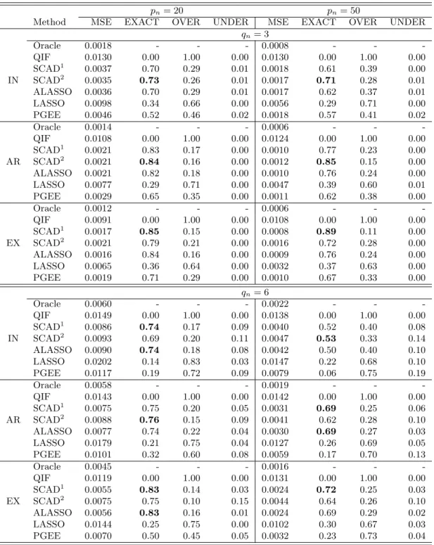
The simulation results from the model selection and the mean square errors (MSE) of estimation are provided in Table 2.1. Table 2.1 illustrates the performance of the penalized QIF approach with the penalty functions of LASSO, adaptive LASSO (ALASSO), and SCAD. The SCAD penalty for the penalized QIF was carried out as SCAD1 through a local quadratic approximation, and SCAD2 through a linear approximation. We compare the penalized QIF to the penalized GEE using the SCAD penalty from 100 simulation runs. In addition, we also provide the standard QIF without penalization (QIF) and the QIF approach based on the oracle model (Oracle) that assumes the true model is known. Table 2.1 provides the proportions of times selecting only the relevant variables (EXACT), the relevant variables plus others (OVER), and only some relevant variables (UNDER). To illustrate estimation efficiency, we took MSE =P100
i=1kβˆ(i)−βk2/100q,where ˆβ(i)is the estimator
from theith simulation run,β is the true parameter,q is the dimension ofβ, andk · kdenotes the Euclidean-norm.
Table 2.1 indicates that the penalized QIF methods based on SCAD1, SCAD2, and ALASSO select the correct model with higher frequencies and smaller MSEs under any working correlation structure. Specifically, SCAD1 performs better than SCAD2 in terms of EXACT and MSE under the true correlation structure, and SCAD1 and SCAD2 perform similarly under the misspecified correlation structures (except when pn = 50 and qn = 3). The performance of SCAD1 and the adaptive LASSO are quite comparable under any working correlation structure. In contrast, the PQIF using the LASSO penalty tends to overfit the model, and its MSEs are much larger compared to the others under any setting. In addition, the MSEs of the PGEE estimators are all greater than those of SCAD1and ALASSO, and the EXACT frequencies of selecting the true models using
PGEE with the SCAD penalty are lower than those of the PQIF based on the SCAD and ALASSO penalties.
When the number of relevant variables doubles, the EXACT of the PQIF based on SCAD and ALASSO decreases about 18% in the worst case; however, the EXACT of the PGEE decreases much more significantly. In the worst case whenqn= 6 andpn= 50, the PGEE selects the correct model less than 25% of the time under any working correlation structure. In addition, the proposed model selection performance is always better under the true correlation structure. For instance, the EXACT is around 70% under the true correlation structure, while it is around 50% under the independent structure when qn= 6 andpn= 50. This simulation also indicates that the proposed model selection method starts to break down when both qn and pn increase under misspecified correlation structures such as the independent structure.
In summary, our simulation results show that the penalized QIF approaches with the SCAD and ALASSO penalties outperform the penalized GEE with the SCAD under any given correlation structure for various dimension settings of parameters in general. The LASSO penalty is not competitive for model selection with diverging number of parameters. In general, SCAD1 performs better than SCAD2, because the linear approximation of SCAD2 is for the first (dominant) term of the PQIF, while the quadratic approximation of SCAD1 is for the second.
2.5.2 Periodontal Disease Data Example
We illustrate the proposed penalized QIF method through performing model selection for an obser-vational study of periodontal disease data (Stoner, 2000). The data contain patients with chronic periodontal disease who have participated in a dental insurance plan. Each patient had an initial periodontal exam between 1988 and 1992, and was followed annually for ten years. The data set consists of 791 patients with unequal cluster sizes varying from 1 to 10.
The binary response variable yij = 1 if the patient i at jth year has at least one surgical tooth extraction, and yij = 0 otherwise. There are 12 covariates of interest: patient gender (gender), patient age at time of initial exam (age), last date of enrollment in the insurance plan in fractional years since 1900 (exit), number of teeth present at time of initial exam (teeth), number of diseased sites (sites), mean pocket depth in diseased sites (pddis), mean pocket depth in all sites
(pdall), year since initial exam (year), number of non-surgical periodontal procedures in a year (nonsurg), number of surgical periodontal procedures in a year (surg), number of non-periodontal dental treatments in a year (dent), and number of non-periodontal dental preventive and diagnostic procedures in a year (prev). Although the variable exit is not related to the model selection, we included it as a null variable to examine whether it is selected by the proposed model selection procedures or not. The logit link function was imposed here for the binary responses.
We minimized the penalized QIF with the SCAD penalty applying the local quadratic approx-imation and the adaptive LASSO penalty to compare with the penalized GEE. Here the AR-1 working correlation structure was assumed for estimation and model selection; as each patient was followed up annually, the measurements are less likely to be correlated if they are further away in time. Although other types of working correlation structure can be applied to these data, the results are not reported here as the outcomes are quite similar. Based on the penalized QIF, we selected relevant covariates asage,sites,pddis,pdall, anddent. The rest of the covariates were not selected and exit was not selected, as expected.
We compare the penalized QIF with the penalized GEE approach (Wang, Zhou, and Qu, 2012) based on the AR-1 working correlation structure. The estimated coefficients of both methods are reported in Table 2.2 indicating that the coefficients ofage,pddis,pdall, and dent are positive and the coefficient of the variablesites is negative. The penalized GEE selects the covariateteeth, while the penalized QIF does not. Overall, the results of the two methods for the periodontal disease data are quite comparable.
In order to evaluate the model selection performance when the dimension of covariates increases, we generated an additional 15 independent null variables from a Uniform (0, 1) distribution. We applied the penalized QIF and the penalized GEE based on the AR-1 working correlation structure. Out of 100 runs, the penalized QIF selected at least one of fifteen null variables 11 times for the SCAD penalty and 13 times for the adaptive LASSO penalty, while the penalized GEE selected one of the null variables 36 times. Furthermore, the penalized QIF always selected the relevant covariatesage,sites,pddis,pdall, anddent, while the penalized GEE selected three other covariates
year,nonsurg, andprev twice, in addition to the 6 relevant variables, in 100 runs. In this example, the penalized GEE tended to overfit the model.
2.6
Discussion
We propose a penalized quadratic inference function approach that enables one to perform model se-lection and parameter estimation simultaneously for correlated data in the framework of a diverging number of parameters. Our procedure is able to take into account correlation from clusters without specifying the full likelihood function or estimating the correlation parameters. The method can easily be applied to correlated discrete responses as well as to continuous responses. Furthermore, our theoretical derivations indicate that the penalized QIF approach is consistent in model selection and possesses the oracle property. Our Monte Carlo simulation studies show that the penalized QIF outperforms the penalized GEE, selecting the true model more frequently.
It is important to point out that the first part of the objective function in the penalized GEE is the generalized estimating equation that is exactly 0 if there is no penalization. This imposes limited choices for selecting a tuning parameter as there is no likelihood function available. Consequently, the PGEE can only rely on the GCV as a tuning parameter selection criterion, which tends to overfit the model. By contrast, the first part of the PQIF is analog to minus twice the log-likelihood function, and therefore can be utilized for tuning parameter selection. We develop a BIC-type criterion for selecting a proper tuning parameter which leads to consistent model selection and estimation for regression parameters. It is also known that the BIC-type of criterion performs better than the GCV when the dimension of parameters is high (Wang, Li, and Leng, 2009). Therefore it is not surprising that the proposed model selection based on the BIC-type of criterion performs well in our numerical studies.
The proposed method is generally applicable for correlated data as long as the correlated mea-surements have the same correlation structure between clusters. This assumption is quite standard for marginal approaches, where the diagonal marginal variance matrix could be different for different clusters, but the working correlation matrix is common for different clusters. When each subject is followed at irregular time points, we can apply semiparametric modeling and nonparametric functional data approaches, but this typically requires more data collection from each subject.
Recent work on handling irregularly observed longitudinal data includes Fan, Huang, and Li (2007) and Fan and Wu (2008) based on semiparametric modeling, and functional data such as James and Hastie (2001); James and Sugar (2003); Yao, M¨uller, and Wang (2005); Hall, M¨uller,
and Wang (2006) and Jiang and Wang (2010). However, most of these are not suitable for discrete longitudinal responses. In addition, semiparametric modeling requires parametric modeling for the correlation function. A disadvantage of the parametric approach for the correlation function is that the estimation of the correlation might be nonexistent or inconsistent if the correlated structure is misspecified. To model the covariance function completely nonparametrically, Li (2011) develops the kernel covariance model in the framework of a generalized partially linear model and transforms the kernel covariance estimator into a positive semidefinite covariance estimator through spectral decomposition. Li’s (2011) approach could be applicable for our method on dealing with irregularly observed longitudinal data, but further research on this topic is needed.
2.7
Proofs of Theorems and Lemmas
Lemma 2.3If (D) holds, An(βn) = E{n−1∇Qn(βn)}= 0 and 1 n∇Qn(βn) =op(1).
ProofBy Chebyshev’s inequality it follows that, for any,
P 1 n∇Qn(βn)−An(βn) ≥ ≤ 1 n2E pn X i=1 ∂Qn(βn) ∂βni −E ∂Qn(βn) ∂βni 2 =pn/n=op(1).
Lemma 2.4Under (D), we have
1 n∇ 2Qn(βn)−Dn(βn) =op(p−n1).
ProofBy Chebyshev’s inequality it follows that, for any,
P 1 n∇ 2Qn(βn)−Dn(βn) ≥ pn ≤ p 2 n n2E pn X i,j=1 ∂2Qn(βn) ∂βni∂βnj −E ∂2Qn(βn) ∂βni∂βnj 2 =p4n/n=op(1).
Lemma 2.5 Suppose the penalty function Pλn(|βn|) satisfies (A), the QIF Qn(βn) satisfies
(D)-(F), and there is an open subset ωqn of Ωqn ∈R
qn that contains the true non-zero parameter point
βs∗. When λn → 0, pn/pnλn → ∞ and p4n/n → 0 as n → ∞, for all the βs ∈ ωqn that satisfy
kβs−βs∗k=Op(ppn/n) and any constantK,
S{(βsT,0)T}=minkβ
sck≤K(
√
pn/n)S{(βs
T, βT
sc)T}, with probability tending to 1.
Proof We take n = K p
pn/n. It is sufficient to prove that, with probability tending to 1 as n→ ∞, for all theβs that satisfyβs−β∗s =Op(
p pn/n), we have for j=qn+ 1, ..., pn, ∂Sn(βn) ∂βnj >0 for 0< βnj < n, ∂Sn(βn) ∂βnj <0 for −n< βnj <0. By the Taylor expansion,
∂Sn(βn) ∂βnj = ∂Qn(βn) ∂βnj +nP 0 λn(|βnj|)sign(βnj) =∂Qn(β ∗ n) ∂βnj + pn X l=1 ∂2Qn(βn∗) ∂βnj∂βnl(βnl−β ∗ nl) + pn X l,k=1 ∂3Qn( ˙βn) ∂βnj∂βnl∂βnk(βnl−β ∗ nl)(βnk−βnk∗ ) +nPλ0n(|βnj|)sign(βnj) =I1+I2+I3+I4,
where ˙βnlies between βn and βn∗, and a standard argument gives
I1 =Op(
√
n) =Op(
√
The second term I2 is I2 = pn X l=1 ∂2Q n(β∗n) ∂βnj∂βnl −E ∂2Q n(βn∗) ∂βnj∂βnl (βnl−βnl∗) + pn X l=1 1 nE ∂2Q n(βn∗) ∂βnj∂βnl n(βnl−βnl∗) =H1+H2. Under (D), we obtain pn X l=1 ∂2Qn(βn∗) ∂βnj∂βnl −E ∂2Qn(βn∗) ∂βnj∂βnl 21/2 =Op( √ npn), and by kβn−βn∗k=Op( p pn/n), it follows that H1=Op( √ npn).Moreover, |H2|= pn X l=1 1 nE ∂2Qn(βn∗) ∂βnj∂βnl n(βnl−βnl∗ ) ≤nOp(1)Op(ppn/n) =Op(√npn). This yields I2 =Op( √ npn). (A.2) We can write I3 = pn X l,k=1 ∂3Qn( ˙βn) ∂βnj∂βnl∂βnk −E ∂3Qn( ˙βn) ∂βnj∂βnl∂βnk (βnl −βnl∗ )(βnk −βnk∗ ) + pn X l,k=1 E ∂3Qn( ˙βn) ∂βnj∂βnl∂βnk (βnl−βnl∗)(βnk−βnk∗ ) =H3+H4.
By the Cauchy-Schwarz inequality, we have
H32 ≤ pn X l,k=1 ∂3Qn( ˙βn) ∂βnj∂βnl∂βnk −E ∂3Qn( ˙βn) ∂βnj∂βnl∂βnk 2 kβn−βn∗k4.
Under (E) and (F),
H3 =Op n np2np 2 n n2 1/2o =Op np4 n n 1/2o =op(√npn). (A.3)
On the other hand, under (E), |H4| ≤K11/2p2nkβn−β ∗ nk2≤K 1/2 1 npnkβn−β ∗ nk2=Op(p2n) =op( √ npn). (A.4)
From (A.1)-(A.4) we have ∂Sn(βn) ∂βnj =Op( √ npn) +Op( √ npn) +op( √ npn) +nPλ0n(|βnj|)sign(βnj) =nλn P0 λn(|βnj|) λn sign(βnj) +Op √pn √ nλn . By (A) and √ pn √ nλn →0, the sign of ∂Sn(βn)
∂βnj is entirely determined by the sign ofβnj.
Proof of Theorem 2.1
Suppose αn = √pn(n−1/2 +an). We want to show that for any given > 0, there exists a constantK such that P
infkuk=KSn(βn∗+αnu)> Sn(βn∗) ≥1−. This implies with probability at least 1− that there exists a local minimum ˆβn in the ball {βn∗ +αnu :kuk ≤ K} such that
kβˆn−βn∗k=Op(αn). We write Gn(u) =Sn(β∗n)−Sn(βn∗ +αnu) =Qn(βn∗)−Qn(βn∗+αnu) +n pn X j=1 {Pλn(|β ∗ nj|)−Pλn(|β ∗ nj+αnuj|)} ≤Qn(βn∗)−Qn(βn∗+αnu) +n qn X j=1 {Pλn(|β ∗ nj|)−Pλn(|β ∗ nj+αnuj|)} =(I) + (II).
By the Taylor expansion,
(I) =−hαn∇TQn(βn∗)u+1 2u T∇2Qn(β∗ n)uα2n+ 1 6∇ T{uT∇2Qn( ˙βn)u}uα3 n i =−I1−I2−I3,
where the vector ˙βn lies betweenβ∗nand βn∗ +αnu, and (II) =− qn X j=1 nαnPλ0n(|βnj∗ |)sign(βnj∗ )uj+nα2nPλ00n(|β∗nj|)u2j{1 +o(1)} =−I4−I5.
By Lemma 2.1 and the Cauchy-Schwarz inequality,I1 is bounded, as
αn∇TQn(βn∗)u≤αnk∇TQn(βn∗)kkuk=Op(
√
npnαn)kuk=Op(nαn2)kuk.
Under (D) and by Lemma 2.2,
I2 = 1 2u T 1 n∇ 2Qn(β∗ n)− 1 nE n ∇2Qn(βn∗)o unα2n+ 1 2u TEn∇2Qn(β∗ n) o uα2n =op(nα2n)kuk2+ nα2n 2 u TD n(βn∗)u.
Under (C) andp2nan→0 asn→ ∞, we have
|I3|= 1 6 pn X i,j,k=1 ∂Qn( ˙βn) ∂βni∂βnj∂βnk uiujukα3n ≤ 1 6n pn X i,j,k=1 M2 1/2 kuk3α3n =Op(p3n/2αn)nα2nkuk3 =op(nα2n)kuk3.
The termsI4 and I5 can be bounded as
|I4| ≤ qn X j=1 |nαnPλ0n(|β ∗ nj|)sign(βnj∗ )uj| ≤nαnan qn X j=1 |uj| ≤nαnan √ qnkuk ≤nα2nkuk and I5 = qn X j=1 nα2nPλ00n(βnj∗ )uj2{1 +o(1)} ≤2max1≤j≤qnP 00 λn(|β ∗ nj|)nα2nkuk2.
For a sufficiently large kuk, all terms in (I) and (II) are dominated by I2. Thus Gn is negative because −I2 <0.
Proof of Theorem 2.2
Theorem 2.1 shows that there is a local minimizer ˆβn ofSn(β) and Lemma 2.3 proves the sparsity property. Next we prove the asymptotic normality. By the Taylor expansion on∇Sn( ˆβs) at point βs∗, we have ∇Sn( ˆβs) =∇Qn(βs∗) +∇2Qn(βs∗)( ˆβs−βs∗) +1 2( ˆβs−β ∗ s)T∇2 ∇Qn( ˙βn) ( ˆβs−βs∗) +∇Pλn(β ∗ s) +∇2Pλn( ¨βn)( ˆβs−β ∗ s),
where ˙βnand ¨βnlie between ˆβs and βs∗. Because ˆβs is a local minimizer,∇Sn( ˆβs) =0,we obtain 1 n ∇Qn(βs∗) +1 2( ˆβs−β ∗ s)T∇2 ∇Qn( ˙βn) ( ˆβs−βs∗) =−1 n h {∇2Qn(βs∗) +∇2Pλn( ¨βn)}( ˆβs−β ∗ s) +∇Pλn(β ∗ s) i . Let Z∼= 12( ˆβs−βs∗)T∇2
∇Qn( ˙βn) ( ˆβs−βs∗) and W ∼=∇2Qn(βs∗) +∇2Pλn( ¨βn). By the
Cauchy-Schwarz inequality and under (E) and (F), we have 1 nZ 2 ≤ 1 n2 n X i=1 nkβˆs−βs∗k4 qn X j,l,k=1 M2 =Op p2 n n2 Op(p3n) =op(n−1). (A.5)
By Lemma 2.2 and under (C) and (F), we obtain
λi n1 nW−Dn(β ∗ s)−Σλn o =op(pn−1/2), fori= 1, ..., qn,
whereλi(B) is theith eigenvalue of a symmetric matrixB. If ˆβs−βs∗ =Op(ppn/n),we have n1 nW−Dn(β ∗ s)−Σλn o ( ˆβs−βs∗) =op(n−1/2). (A.6)
From (A.5) and (A.6) we obtain
{Dn(β∗s) +Σλn}( ˆβs−β ∗ s) +bn=− 1 n∇Qn(β ∗ s)−op(n−1/2), (A.7)
and from (A.7) we have √ nBnD−n1/2(βs∗){Dn(βs∗) +Σλn} ( ˆβs−βs∗) +{Dn(βs∗) +Σλn} −1b n =√nBnD−n1/2(β∗s){Dn(βs∗) +Σλn}( ˆβs−β ∗ s) +bn =−√1 nBnD −1/2 n (βs∗)∇Qn(βs∗)−op{BnD−n1/2(β∗s)}. As the last term is op(1), we only consider the first term denoted by
Yni= 1 √ nBnD −1/2 n (βs∗)∇Qni(βs∗), fori= 1, ..., n.
We show that Yni satisfies the conditions of the Lindeberg-Feller Central Limit Theorem. By Lemma 2.1, (D), andBnBTn →F, we have
EkYn1k4 = 1 n2EkBnD −1/2 n (βs∗)∇Qni(βs∗)k4 ≤ 1 n2λmax(BnB T n)λmax{Dn(βs∗)}Ek∇TQn(βs∗)∇Qn(βs∗)k2 = O(p2nn−2), (A.8)
and by Chebyshev’s inequality
P(kYn1k> )≤ EkYn1k2 ≤ EkBnD−n1/2(βs∗)∇Qni(βs∗)k2 n =O(n −1). (A.9)
From (A.8) and (A.9) andp4n/n→0 as n→ ∞, we obtain n
X i=1
EkYnik21{kYnik> } ≤n{EkYn1k4}1/2{P(kYn1k> )}1/2
On the other hand, as BnBnT →F we have n
X i=1
cov(Yni) =n·cov(Yn1) =cov{BnD−n1/2(β
∗
s)∇Qn(β
∗
s)} →F.
It follows that the Lindeberg condition is satisfied and then the Lindeberg-Feller central limit theorem gives √ nBnD−n1/2(βs∗){Dn(βs∗) + Σλn} ( ˆβs−βs∗) +{Dn(βs∗) +Σλn} −1b n d →N(0, F). Proof of Lemma 2.1 Let ˆβnλo = ( ˆβ T sλo, ˆ βsTcλ o) T be an estimator ofβ
n= (βsT, βsTc)T.The oracle property of the penalized
QIF ensures that, with probability tending to 1, ˆβsλo satisfies
S0n( ˆβsλo) =Q 0 n( ˆβsλo) +bn( ˆβsλo) = 0, (A.10) wherebn={Pλ0n(|βn1|)sign(βn1), ..., P 0 λn(|βnqn|)sign(βnqn)} T.By (F),P(|βˆ sλo|> aλo)−→1,which
implies that P(bn( ˆβsλo) = 0) −→ 1. Therefore with probability tending to 1, (A.10) leads to
Q0n( ˆβsλo) = 0. This implies that ˆβsλo is the same as ˆβ
∗
s, the oracle estimator for the non-zero coefficients. It immediately follows that, with probability tending to 1, BIQIFλo = Q
0
n( ˆβsλo) +
qnlog(n) =Q0n( ˆβs∗) +qnlog(n) =BIQIFΥT.
Proof of Lemma 2.2
The proof of Lemma 2.2 consists of different cases for underfitted or overfitted models. We show that Lemma 2.2 holds for each case.
For underfitted models, it follows by Lemma 2.1 that BIQIFλo n = ¯gn( ˆβλo) TC¯−1 n ( ˆβλo)¯gn( ˆβλo) +qn log(n) n P −→¯gn(βΥT) TC¯−1 n (βΥT)¯gn(βΥT).
In addition, since Υλ +ΥT, we have BIQIFλn n = ¯gn( ˆβλn) TC¯−1 n ( ˆβλn)¯gn( ˆβλn) +dfλn log(n) n ≥gn¯ ( ˆβλn) TC¯−1 n ( ˆβλn)¯gn( ˆβλn) ≥minΥ:Υ+ΥTgn¯ ( ˆβΥ)TC¯n−1( ˆβΥ)¯gn( ˆβΥ) P −→minΥ:Υ+ΥTg¯n(βΥ)TC¯n−1(βΥ)¯gn(βΥ)>¯gn(βΥT) TC¯−1 n (βΥT)¯gn(βΥT). Therefore, P(infλn∈Λ− BIQIFλn n > BIQIFλo
n ) =P(infλn∈Λ−BIQIFλn > BIQIFλo)−→1.
For overfitted models, we have
infλn∈Λ+(BIQIFλn−BIQIFλo) = infλn∈Λ+(Qn( ˆβλn)−Qn( ˆβλo) + (dfλn−qn)) log(n)
≥infλn∈Λ+(Qn( ˆβλn)−Qn( ˆβλo)) + log(n)
≥minΥ:Υ⊃ΥT(Qn( ˆβΥ)−Qn( ˆβΥT)) + log(n).
SinceQn( ˆβΥ)−Qn( ˆβΥT) has an asymptoticχ
2
dfΥ−qn distribution, minΥ:Υ⊃ΥT(Qn( ˆβΥ)−Qn( ˆβΥT)) =
Op(1) and, with log(n) divergent, we have P(infλn∈Λ+BIQIFλn > BIQIFλo) −→1.
Online Supplementary Materials
The R-coding for simulation studies for binary responses is given in the online supplemental material available at http://www.stat.sinica.edu/statistica.
Table 2.1: Performance of penalized QIF with LASSO, adaptive LASSO (ALASSO), SCAD1, SCAD2, and penalized GEE (PGEE) using SCAD penalty, with three working correlation struc-tures: IN (independent), AR (AR-1) and EX (exchangeable).
pn= 20 pn= 50
Method MSE EXACT OVER UNDER MSE EXACT OVER UNDER
qn= 3 Oracle 0.0018 - - - 0.0008 - - -QIF 0.0130 0.00 1.00 0.00 0.0130 0.00 1.00 0.00 SCAD1 0.0037 0.70 0.29 0.01 0.0018 0.61 0.39 0.00 IN SCAD2 0.0035 0.73 0.26 0.01 0.0017 0.71 0.28 0.01 ALASSO 0.0036 0.70 0.29 0.01 0.0017 0.62 0.37 0.01 LASSO 0.0098 0.34 0.66 0.00 0.0056 0.29 0.71 0.00 PGEE 0.0046 0.52 0.46 0.02 0.0018 0.57 0.41 0.02 Oracle 0.0014 - - - 0.0006 - - -QIF 0.0108 0.00 1.00 0.00 0.0124 0.00 1.00 0.00 SCAD1 0.0021 0.83 0.17 0.00 0.0010 0.77 0.23 0.00 AR SCAD2 0.0021 0.84 0.16 0.00 0.0012 0.85 0.15 0.00 ALASSO 0.0021 0.82 0.18 0.00 0.0010 0.76 0.24 0.00 LASSO 0.0077 0.29 0.71 0.00 0.0047 0.39 0.60 0.01 PGEE 0.0029 0.65 0.35 0.00 0.0011 0.62 0.38 0.00 Oracle 0.0012 - - - 0.0006 - - -QIF 0.0091 0.00 1.00 0.00 0.0108 0.00 1.00 0.00 SCAD1 0.0017 0.85 0.15 0.00 0.0008 0.89 0.11 0.00 EX SCAD2 0.0021 0.79 0.21 0.00 0.0016 0.72 0.28 0.00 ALASSO 0.0016 0.84 0.16 0.00 0.0009 0.76 0.24 0.00 LASSO 0.0065 0.36 0.64 0.00 0.0032 0.37 0.63 0.00 PGEE 0.0019 0.71 0.29 0.00 0.0010 0.67 0.33 0.00 qn= 6 Oracle 0.0060 - - - 0.0022 - - -QIF 0.0149 0.00 1.00 0.00 0.0138 0.00 1.00 0.00 SCAD1 0.0086 0.74 0.17 0.09 0.0040 0.52 0.40 0.08 IN SCAD2 0.0093 0.69 0.20 0.11 0.0047 0.53 0.33 0.14 ALASSO 0.0090 0.74 0.18 0.08 0.0042 0.50 0.40 0.10 LASSO 0.0202 0.14 0.83 0.03 0.0147 0.22 0.68 0.10 PGEE 0.0117 0.19 0.72 0.09 0.0079 0.06 0.75 0.19 Oracle 0.0058 - - - 0.0019 - - -QIF 0.0143 0.00 1.00 0.00 0.0142 0.00 1.00 0.00 SCAD1 0.0075 0.75 0.20 0.05 0.0031 0.69 0.25 0.06 AR SCAD2 0.0088 0.76 0.15 0.09 0.0041 0.62 0.28 0.10 ALASSO 0.0077 0.74 0.22 0.04 0.0030 0.69 0.27 0.03 LASSO 0.0179 0.21 0.75 0.04 0.0127 0.26 0.69 0.05 PGEE 0.0101 0.32 0.60 0.08 0.0059 0.17 0.70 0.13 Oracle 0.0045 - - - 0.0016 - - -QIF 0.0119 0.00 1.00 0.00 0.0131 0.00 1.00 0.00 SCAD1 0.0055 0.83 0.14 0.03 0.0024 0.72 0.25 0.03 EX SCAD2 0.0075 0.75 0.10 0.15 0.0044 0.64 0.26 0.10 ALASSO 0.0056 0.83 0.16 0.01 0.0024 0.69 0.29 0.02 LASSO 0.0144 0.25 0.75 0.00 0.0102 0.30 0.67 0.03 PGEE 0.0070 0.50 0.45 0.05 0.0032 0.23 0.73 0.04
Table 2.2: For the periodontal disease study, the coefficients estimated by the unpenalized QIF (QIF), the penalized QIF with SCAD through a local quadratic approximation (SCAD), the adap-tive LASSO (ALASSO), the unpenalized GEE (GEE), and the penalized GEE (PGEE).
QIF SCAD ALASSO GEE PGEE
intercept -8.284 -11.144 -10.824 -8.287 -9.125 gender -0.002 0.000 0.000 0.034 0.000 age 0.016 0.009 0.006 0.012 0.009 exit -0.032 0.000 0.000 -0.002 0.000 teeth 0.000 0.000 0.000 -0.027 -0.014 sites -0.006 -0.006 -0.005 0.000 -0.003 pddis 0.704 0.715 0.605 0.567 0.545 pdall 0.833 0.871 0.826 0.551 0.668 year 0.018 0.000 0.000 -0.021 0.000 nonsurg 0.004 0.000 0.000 -0.039 0.000 surg 0.018 0.000 0.000 0.015 0.000 dent 0.124 0.115 0.128 0.110 0.106 prev -0.152 0.000 0.000 -0.147 0.000
Chapter 3
Consistent Moment Selection from
High-Dimensional Moment
Conditions
3.1
Introduction
The generalized method of moments (GMM, Hansen, 1982) is widely applicable when the likelihood function is difficult to specify, while moment conditions are easy to formulate. The GMM is powerful as it optimally combines valid moment conditions and is able to achieve estimation efficiency. However, the GMM could perform poorly if there are too many moment conditions relative to the sample size, due to limitation in finite samples (Newey and Smith, 2004). We are motivated by the problem where the dimension of estimating equations or moment conditions far exceeds the sample size. For example, in modeling dynamic panel data, a large dimension of valid moment conditions can be generated based on the first-order moments (Anderson and Hsiao, 1981; Han, Orea, and Schmidt, 2005; Han and Phillips, 2006). For longitudinal data, the dimension of moment conditions depends on the number of basis matrices to approximate an inverse of the correlation matrix (Qu, Lindsay, and Li, 2000), which can be larger than the sample size.
The key component of the GMM is the optimal weighting matrix, which is the inverse of the sample covariance matrix of moment conditions. However, the sample covariance matrix could be problematic when the dimension is large due to the following two reasons: i) the sample covariance matrix is not of full rank if the dimension of moment conditions exceeds the sample size; ii) even if the sample covariance matrix is invertible, the estimation of its inverse could be biased with high variation when the number of moment conditions is close to the sample size. Donald and Newey (2001) and Donald, Imbens, and Newey (2009) proposed selecting moment conditions based on the criterion of minimizing the mean square error of the estimator. However, their criterion involves inverting the sample covariance matrix, which could be infeasible if the covariance matrix
is ill-conditioned, as indicated in the above two cases.
In recent years, estimating the covariance matrix Σ and its inverse has drawn a lot of attention for the high-dimensional data setting. For example, Bickel and Levina (2008), Rothman, Levina, and Zhu (2009) and Cai and Liu (2011) proposed element-wise shrinkage and thresholding pro-cedures to estimate Σ−1. Meinshausen and B¨uhlmann (2006) introduced neighborhood selection for high-dimensional graphs via the lasso penalty. In addition, Friedman, Hastie, and Tibshirani (2007), Peng et al. (2009), Witten, Friedman, and Simon (2011) and Danaher, Wang, and Witten (2012) solved the graphical lasso problem through estimating the precision matrix Σ−1. Most of these methods utilize sparsity structure assuming that the majority of off-diagonal elements are zero; however, they do not provide strategies for solving the matrix singularity problem.
To estimate the large dimensional covariance matrix under a more general framework without sparsity assumptions, various dimension reduction strategies through matrix decomposition have been proposed. For example, Wu and Pourahmadi (2003), Huang et al. (2006) and Pourahmadi (2007) employed regularized regression based on a modified Cholesky decomposition; Magdon-Ismail and Purnell (2011) applied a low-rank perturbation of a diagonal matrix to estimate Σ−1
for a Gaussian mixture model; and Fan, Fan, and Lv (2008) and Fan, Liao, and Mincheva (2011) developed a factor model to estimate the invertible covariance matrix. In addition, Luo (2011) proposed a general framework for low-rank approximation and sparse covariance structures simul-taneously. However, these methods do not directly address how to extract important information from a large-dimensional matrix which is either singular or close to singular.
The singularity problem of the sample covariance makes the GMM estimator infeasible or un-stable. When there are many valid moment conditions available, subset moment selection methods have been developed. Gallant and Tauchen (1996), Andrews and Lu (2001), Donald and Newey (2001), Donald, Imbens, and Newey (2009) and Okui (2009) proposed to eliminate the least use-ful moment conditions to reduce the overall number of moment conditions. However, selecting a subset of moment conditions requires prior information of the moment conditions. In addition, information from the unselected moment conditions is lost for parameter estimation.
To circumvent this problem, Doran and Schmidt (2006) proposed to combine all available moment conditions using principle components analysis. They apply spectral decomposition of