2017
Learning Markov Logic Network Structure by
Template Constructing
Yingbei Tong
Iowa State UniversityFollow this and additional works at:
https://lib.dr.iastate.edu/etd
Part of the
Computer Sciences Commons
This Thesis is brought to you for free and open access by the Iowa State University Capstones, Theses and Dissertations at Iowa State University Digital Repository. It has been accepted for inclusion in Graduate Theses and Dissertations by an authorized administrator of Iowa State University Digital Repository. For more information, please [email protected].
Recommended Citation
Tong, Yingbei, "Learning Markov Logic Network Structure by Template Constructing" (2017).Graduate Theses and Dissertations. 15441.
Yingbei Tong
A thesis submitted to the graduate faculty
in partial fulfillment of the requirements for the degree of MASTER OF SCIENCE
Major: Computer Science
Program of Study Committee: Jin Tian, Major Professor
Carl Chang Pavan Aduri
Iowa State University Ames, Iowa
2017
DEDICATION
I would like to thank my family and friends for their loving guidance and financial assistance during the writing of this work.
TABLE OF CONTENTS LIST OF TABLES . . . v LIST OF FIGURES . . . vi ACKNOWLEDGEMENTS . . . vii ABSTRACT . . . viii CHAPTER 1. OVERVIEW . . . 1 1.1 Introduction . . . 1 CHAPTER 2. BACKGROUND . . . 3 2.1 First-order logic . . . 3 2.2 Markov networks . . . 4
2.3 Markov logic networks . . . 6
2.3.1 Inference . . . 8
2.3.2 Structure learning . . . 8
CHAPTER 3. TEMPLATE CONSTRUCTING STRUCTURE LEARNING 10 3.1 Construct template nodes . . . 10
3.2 Generate observations . . . 13
3.3 Alternative approach to create template nodes and observations . . . 14
3.4 Learn the template and build candidate clauses . . . 15
CHAPTER 4. EXPERIMENTAL EVALUATION . . . 18
4.1 Experimental setup . . . 18
4.1.1 Datasets . . . 18
4.1.2 Methodology . . . 18
CHAPTER 5. CONCLUSION AND FUTURE WORK . . . 21 REFERENCES . . . 22
LIST OF TABLES
Table 2.1 Example of a MLN . . . 7
Table 3.1 Example database . . . 12
Table 3.2 Template nodes constructed . . . 13
Table 3.3 An example of observations generated . . . 14
Table 4.1 Details of dataset . . . 18
Table 4.2 Experimental results of AUCs . . . 20
LIST OF FIGURES
Figure 2.1 An example Markov network . . . 5
Figure 2.2 Ground Markov network . . . 7
ACKNOWLEDGEMENTS
I would like to take this opportunity to express my thanks to those who helped me with various aspects of conducting research and the writing of this thesis. First and foremost, Dr. Tian for his guidance, patience and support throughout this research and the writing of this thesis. His insights and words of encouragement have often inspired me and renewed my hopes for completing my graduate education. I would also like to thank my committee members for their efforts and contributions to this work: Dr. Chang and Dr. Aduri.
ABSTRACT
Markov logic networks (MLNs) are a statistical relational model that incorporates first-order logic and probability by attaching weights to first-first-order clauses. However, due to the large search space, the structure learning of MLNs is a computationally expensive problem. In this paper, we present a new algorithm for learning the structure of Markov Logic Network by directly utilizing the data to construct the candidate clauses. Our approach makes use of a Markov Network learning algorithm to construct a template network. We then apply the template to guide the candidate clauses construction process. The experimental results demonstrate that our algorithm is promising.
CHAPTER 1. OVERVIEW
1.1 Introduction
In recent years, there has been an increasing interest in methods for unifying the strengths of first-order logic and probabilistic graphical models in machine learning area (Getoor and Taskar, 2007). Markov Logic Networks (MLNs) are a statistical relational model that combine first-order logic and Markov networks. An MLN typically consists of a set of first-order clauses attached with weights, and it can be viewed as a template for features of Markov networks (Richardson and Domingos, 2006). Learning a MLN can be decomposed into two separated parts: structure learning (learning the logical clauses) and weight learning (learning the weight of each clause). Learning the structure of a MLN is the process of generating a set of clauses attached with their weights (Kok and Domingos, 2005), and it allows us to obtain uncertain dependencies underlying the relational data.
The structure learning problem of MLNs is an important but challenging task. With the continuous increasing of the data size, the search space is usually super-exponentially large and the clause evaluation also generates huge amount of groundings. In general, search for all the possible candidate clauses and evaluate them with full groundings may not be a feasible solution. A few practical approaches have been proposed to date, among which the MSL (Kok and Domingos, 2005), BUSL (Mihalkova and Mooney, 2007), ILS (Biba et al., 2008b), LHL (Kok and Domingos, 2009), LSM (Kok and Domingos, 2010), HGSM (Dinh et al., 2010b), GSLP (Dinh et al., 2011) and LNS (Sun et al., 2014). Most of these approaches focus on constraining the search space of the candidate clauses in a top-down or bottom-up manner.
The top-down approaches follow a general-and-test strategy, start from an empty clause, systematically enumerate candidate clauses by greedily adding literals to existing clauses, and evaluate the result clauses’ empirical fit to training data by using some scoring models. Such
approaches are usually inefficient as they have two shortcomings: searching the explosive space of clauses is computationally expensive; and it is susceptible to result in a local optimum. Bottom-up approaches, however, overcome these limitations by directly utilizing the training data to construct candidate clauses and guide the search.
In this paper, we present a novel MLN structure learning algorithm. This algorithm first constructs a set of template nodes from the database, then creates a set of observations using the data , and utilize the template nodes and observations to learn a ”template” Markov networks. This template is then applied to guide the candidate clauses construction process. Candidate clauses are evaluated and reduced to form the final MLN.
We begin the paper by briefly reviewing the necessary background knowledge of first-order logic, Markov networks, and Markov logic networks in chapter 2. We then describe the details of our structure learning algorithms in chapter 3, and report the experimental results in chapter 4. Last, we conclude this paper and discuss future work in chapter 5.
CHAPTER 2. BACKGROUND
In this chapter, we explain the necessary background knowledge about Markov logic net-works. We start with first-order logic and Markov network, then we introduce how Markov logic network incorporates them together. Finally, we demonstrate the structure learning problem of MLNs and review some previous works.
2.1 First-order logic
A first-order knowledge base (KB) is a set of formulas or sentences in first-order logic (Genesereth and Nilsson, 1987). There are four types of symbols in first-order logic: constants, variables, functions and predicates. Constant symbols represent objects in a domain and can have types (e.g., person: alice, bob, carl,etc.). Variable symbols range over the objects in a domain. Function symbols represent functions that map tuples of objects to objects(e.g.,
M otherOf). Predicate symbols describe attributes of objects (e.g.,Student(clice)) or relations between objects in the domain (e.g., workedU nder(alice, bob)). Constants and variables are often typed, that is, constants can only represent objects of the corresponding type and variables can only range over objects in the corresponding type. In this paper, we assume no functions in the domains. We denote constants by lower-cased strings, variables by single upper-case letters and predicates by strings that start with upper-case letters.
Example: We use the IMDB database as the domain for this example: This dataset
contains facts that describe the profession of individuals in the movie business, relationships
that indicate the connection between people, and themovies represent which person works for which movie. Actor(alice) means alice is an actor and Director(bob) indicates that bob is a director. The predicate workedU nder(A, B) specifies that personA works on a movie under the supervision of person B, and the predicate M ovie(T, C) specifies that person C works on
movieT. Here bothA, B, andT are variables,Aand B range over objects in typePersonand
T range over objects in type Movie.
A term is any expression that represents an object in the domain. It can be a constant, a variable, or a function that is applied to terms. For example, alice,A, and M otherOf(alice) are terms. Ground terms contain no variables. An atomic formula or atom is a predicate applied to a tuple of terms(e.g., workedU nder(alice, M otherOf(alice))). A ground atom is a predicate replaces all variables with constants. We call an atomvariable atomif it only contains variables. Formulas are constructed from atoms using logical connectives and quantifiers. A positive literal is an atom and a negative literal is a negated atom. A clause is a disjunction of positive and negative literals. The number of literals in the disjunction is the length of the clause. Adatabase is a partial specification of a world, that is, each atom in it is true, false or unknown. In this paper, we make a closed-world assumption: a ground atom in the database is assumed to be true, a ground atom that is not in the database is considered false. A world is an assignment of truth values to all the possible ground atoms in a domain.
To conclude, first-order logic is a helpful tool that widely used in Artificial Intelligence area for the purpose of knowledge representation . Its expressiveness allows us to describe the complexity of the world in a more succinct way. However, first-order logic can not handle the uncertainty of the world, thus, pure first-order logic has restricted applicability to practical AI problems.
2.2 Markov networks
A Markov network (orMarkov random field) is an undirected graphical model for the joint distribution of a set of random variables X = (X1, X2, ....Xn) ∈ X (Pearl, 1988). It consists
of an undirected graph G = (V, E) with a list of potential function φk. The graph G has a
set of nodes, each of them represents one of the random variable. Nodes are connected by edges, which describe the dependency of nodes. A clique is a set of nodes, where each pair of nodes in the clique is connected by an edge. For each clique in the graph there is a potential function. Each potential function is a real-valued non-negative function, represents the state of the corresponding clique. Figure2.1 gives an example of a Markov network. There are four
Given a set of random variablesX= (X1, X2, ....Xn)∈ X, letP(X=x) be the probability
of finding that random variableXtakes on the particular value configurationx. BecauseXis a set of variables, thenP(X=x) can be understood to be thejoint distribution ofX. Thejoint distributionfor a Markov network is given by the following formula (Richardson and Domingos, 2006): P(X=x) = 1 Z Y k φk(x{k}) (2.1)
where x{k} is the state of variables that appear in the kth clique. Here Z is the normalizing
partition function given by: Z = P
x∈XQkφk(x{k}). Markov networks can also equivalently
written aslog-linear models, which is given by:
P(X=x) = 1
Zexp( X
k
wkfk(x{k})) (2.2)
wherefk(x{k}) is the feature corresponding tox{k} with its weightwkbeing logφk(x{k}). Each
feature can be any real-valued function of the state, but in this paper we will only focus on binary features, that is, it is either 0 or 1, depends on whether it is satisfied or not.
Figure 2.1 An example Markov network
Markov network is a probabilistic model that handles the uncertainty of the world. However, it is not expressiveness and can not describe the complexity of the world.
2.3 Markov logic networks
Markov Logic network is a statistical relational learning model that unifies first-order logic and Markov network, takes the advantages from both of them. It consists of a set of weighted first-order clauses. If we consider a first-order KB as a set of hard constraints on the possible worlds, then a MLN can be seen as an approach to soften these constraints: a world that violates some clauses is less likely to be possible, but not impossible. The fewer clauses a world violates, the more probable it is. The weight attached to a clause shows how strong the constraint is. A higher weight indicates the greater difference between a world satisfies the clauses and the world that does not. Table2.1shows an example of a simple MLN. The formal definition of MLNs is defined as follows:
Definition 1(Richardson and Domingos, 2006) A Markov logic networkLis a set of pairs (fi, wi), where fi is a formula in first-order logic and wi is a real number. Together with a
finite set of constantsC ={c1, c2, ..., c|C|}, it defines a Markov network ML,C (2.1and 2.2) as
follows:
1. ML,C contains one binary node for each possible grounding of each atom appearing in L. The value of the node is 1 if the grounding atom is true, and 0 otherwise.
2. ML,C contains one feature for each possible grounding of each formulafiinL. The value
of this feature is 1 if the ground formula is true, and 0 otherwise. The weight of the feature is thewi, attached withfi inL.
Two nodes inML,C are connected by an edge if and only if the corresponding ground atoms
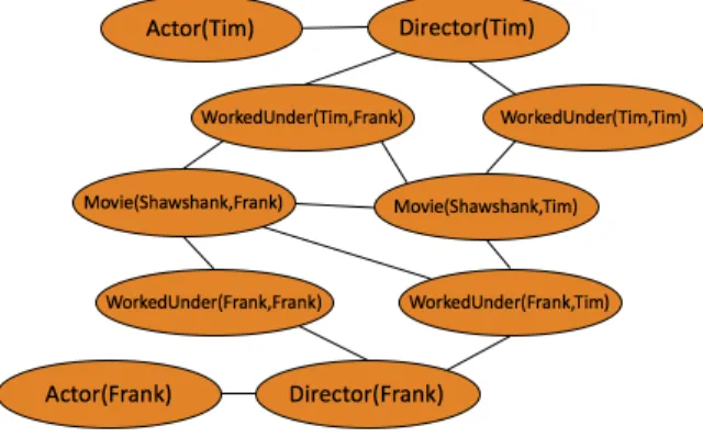
appear together in some ground formulas in L. Thus the atoms in each ground formula form a clique in ML,C. For example, figure 2.2 shows the graph of the ground Markov network
defined by giving the MLN in table 2.1 with constants T im, F rank, and Shawshank. This graph contains a node for each ground atom and an edge for each pair of atoms that appear together in one of the ground formula. Its features include Actor(T im) ⇒ ¬Director(T im),
Director(F rank)⇒ ¬W orkedU nder(F rank, T im), etc.
An MLN can be seen as a template for generating Markov networks, given different sets of constants, it will construct different ground Markov networks. LetX be the set of all ground atoms, F be the set of all clauses in the MLN, wi be the weight attached with clause fi ∈ F,
Figure 2.2 Ground Markov network
Gfi be the set of all possible groundings of clause fi with the constants in the domain. Then
the probability of a possible worldx specified by the ground Markov network ML,C is defined
as: P(X=x) = 1 Zexp( X fi∈F wi X g∈Gfi g(x)) = 1 Zexp( X fi∈F wini{x}) (2.3)
The value of g(x) is 1 if g is satisfied and 0 otherwise. Then, given a truth assignment toX, the quantity P
g∈Gfig(x) counts the number of groundings of fi that are true. Thusni{x} is
the number of true groundings offi inx.
For example, consider an MLN that contains exactly one formulaActor(A)⇒ ¬Director(A) with its weightw, andC ={Bob}. This results in four possible worlds: {Actor(Bob), Director(Bob)}, {¬Actor(Bob), Director(Bob)},{Actor(Bob),¬Director(Bob)}, and{¬Actor(Bob),¬Director(Bob)}. From 2.3 we can obtain P({Actor(Bob), Director(Bob)}) = 3ew1+1 and the probability of the
other three worlds is 3eeww+1. Here 3ew+ 1 is the value of partition functionZ. Thus, anyw >0
will make the world P({Actor(Bob), Director(Bob)}) less possible than the others. Table 2.1 Example of a MLN
First-order logic Weight
Actor(A)⇒ ¬Director(A) 0.8
Director(A)⇒ ¬W orkedU nder(A, B) 1.2
2.3.1 Inference
To perform inference over a given MLN, one needs to ground it to its corresponding Markov network (Pearl, 1988). As described by Richardson and Domingos (2006), this process can be done as follows. First, all the possible ground atoms in the domain are constructed, and they are used as the nodes of the Markov network. The edges in the Markov network are decided by the groundings of the first-order clauses, that is, two ground atoms are connected if they are both in a grounding of a clause. Thus, nodes that participate together in a ground clause will form cliques.
2.3.2 Structure learning
Given a database, the problem of learning a MLN can be separated into two parts: weight learning and structure learning, where structure learning referred to learning the formulas and weight learning referred to learning the weights. In this paper we only focus on the structure learning problem, because given a structure learned, a weight learning algorithm calledL−BF GS (Liu and Nocedal, 1989) has been developed to learn the weights. The main task in learning the structure of MLNs is to find a set of potentially good clauses. Clauses are evaluated using a weighted pseudo log-likelihood (WPLL) measure, introduced in (Kok and Domingos, 2005), defined as:
logPw(X=x) = X r∈R cr gr X k=1 logPw(Xr,k=xr,k|M Bx(Xr,k)) (2.4)
whereR is the set of first-order predicates, gr is the number of groundings of predicater,xr,k
is the truth value (either 0 or 1) of the kth ground atom of r,cr= 1/gr.
Some previous works on structure learning are: MSL, BUSL, listed as follows:
MSL: This algorithm is proposed by Kok and Domingos (2005), it uses beam search to search from all possible clauses. In each iteration, MSL uses beam search to find the best clause, and add it to the MLN: starting with all the unit clauses, it applies each possible operator (addition and deletion) to each clause, keep the n best ones, apply the operator to those, and repeat until no new clause improves the WPLL. The best clause is the one with highest WPLL score and it will be added to the MLN. MSL terminates when no more clause can be added to the MLN, and it then returns the MLN.
the paths as nodes and the boolean value matrix as training data. It utilizes the Grow-Shrink Markov network structure learning algorithm to connect the nodes. After construction of Markov network template, it creates candidate clauses by making disjunctions of the atoms in each clique’s node. Finally, it uses WPLL to evaluate the candidates and discards those candidates that do not increase the overall WPLL.
CHAPTER 3. TEMPLATE CONSTRUCTING STRUCTURE LEARNING
In this chapter, we explain the details of our algorithms: learning Markov logic network structure by template constructing (TCSL).
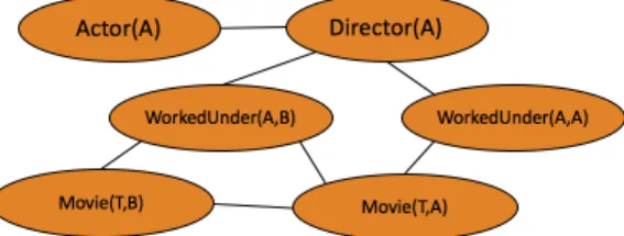
As we mentioned in chapter 2, MLNs can be viewed as templates for generating Markov networks, given different sets of constants, different ground Markov networks are constructed. Thus, we want to create a Markov network template similar to the one in figure 3.1to restrict the search space and guide the construction of candidate clauses. Algorithm1gives the skeleton of TCSL. Let P be the set of all predicates in the domain. Each predicateP is considered in sequence. For eachP, the algorithm first constructs a set of template nodes, and creates a set of observations using the data. A Markov network template is then learned using the template nodes and the observations. Finally, we focus on each maximal clique in the template network and generate a set of candidate clauses. We evaluate the candidates with the WPLL score, add these candidates which increase the overall WPLL score to the final MLN.
Figure 3.1 An example Markov network template
3.1 Construct template nodes
To learn a Template network using Markov network structure learning algorithm, we first need to construct a set of template nodes. A template node is basically a literal that only
2: foreach P ∈ P do
3: Construct template nodes for predicate P
4: Generate observations for the template nodes
5: Use the template nodes and the observations to learn the Markov network template 6: Use the template to build candidate clauses
7: end for
8: Remove duplicate candidates clauses
9: Evaluate candidates, add the best ones toM LN
10: return M LN
contains variables. We use predicate P to create the first template node, referred to as the
headN ode. Other template nodes are then created by searching for constant-shared ground atoms in the database and constructing a corresponding variable literal. Thus, template nodes are actually atoms that have true groundings in the data. The output of template nodes con-struction process for predicateP is an array, which contains a set of template nodes. Algorithm
2 displays how the template nodes are created. It makes use of the following definition:
Definition 2 Two ground atoms are constant-shared or connected if there is at least one constant that is an argument of both.
Let P be the predicate currently under consideration in this iteration,m be the maximum number of free variable that can be allowed in the templateN odeArray. The algorithm first creates the variable atom of P as the headN ode in line 1, and add it to the position 0 of
templateN odeArray. Each argument in headN ode is assigned a unique variable. In line 2, we set variableN um to the number of variables in headN ode. Next, from line 3 to 15, the algorithm iterates over each possible ground atomGP ofP. In line 4, it finds the set of all the
true ground atoms in the data that are constant-shared withGP, denoted asCGP. Then for each
c ∈ CGP, it constructs a new template node. If the newN ode was not created previously and did not violate the limitation of variable number, then it will be added totemplateN odeArray
(line 9-10). However, note that some nodes will be ignored if there already existsm variables, thus some useful information may be lost.
Example: Assume we are given the database shown in table 3.1 as the domain of our
Algorithm 2 TemplateNodesConstruction(P ,m)
Input:
P: the predicate being considered in this loop
m: maximum free variable number allowed in the array
Output:
templateN odeArray: the array contains template nodes
1: Use P to create the head template node, called headNode, and add it to the place 0 of
templateN odeArray.
2: variableN um= number of variables in headN ode
3: for eachGP, ground atom ofP do
4: let CGP be the set of all the true ground atoms that are constant-shared with GP 5: for eachc∈ CGP do
6: newN ode= Create a new template node
7: variableN um+ = new variable introduced in newN ode
8: Index=templateN odeArray.f ind(newN ode) 9: if Index <0&&variableN um <=m then 10: add newN odetotemplateN odeArray
11: else
12: variableN um−= new variable introduced innewN ode
13: end if
14: end for
15: end for
aref alse:
Table 3.1 Example database
Actor(T im)
Director(F rank)
W orkedU nder(T im, F rank)
M ovie(Shawshank, T im)
M ovie(ShawShank, F rank)
Suppose the predicate currently under consideration is P = Actor. Then the headNode is Actor(A). We need to consider each ground atom of P and let’s start with Actor(Tim). The constant-shared ground atoms of Actor(Tim) in the database are WorkedUnder(Tim, Frank) and Movie(Shawshank, Tim). Thus we can create template nodes WorkedUnder(A, B) and Movie(C,A), add them to templateNodeArray. Next we consider the other ground atom Ac-tor(Frank): the constant-shared ground atoms in the database are Director(Frank), WorkedUn-der(Tim, Frank) and Movie(Shawshank, Frank). Template nodes constructed are Director(A)
nodes constructed. There are four free variables in the array: A, B, C and D.
Table 3.2 Template nodes constructed
Actor(A) W orkedU nder(A, B) M ovie(C, A) Director(A) W orkedU nder(D, A)
3.2 Generate observations
We have constructed a list of template nodes and added them to the array. Next we will generate a set of observations for the template nodes. We have limited the number of free variables intemplateN odeArray by setting the parameterm. Algorithm3lists the procedure.
Algorithm 3 Generate Observations
Input:
templateN odeArray : the array of template nodes
m : max free variable number intemplateN odeArray Output:
M : a matrix contains the observations generated
1: letS be the set of all possible assignments to the variables of the template nodes. 2: foreach si∈ S do
3: append a new array M[i] toM
4: for each nodenj ∈templateN odeArray do
5: if the ground atom ofnj under the assignment si istruethen 6: M[i][j] =true 7: else 8: M[i][j] =f alse 9: end if 10: end for 11: end for
LetS be the set of all possible assignments for the variables in thetemplateN odeArray,M
be the result matrix containing a column for each template node and a row for each possible assignment. The algorithm considers each assignmentsi∈ S, it first add a new empty array to M, then, in line 4-8, it checks the ground atom of each template node given variable assignment
si, set the corresponding value in M to true if the ground atom exists in the data and false
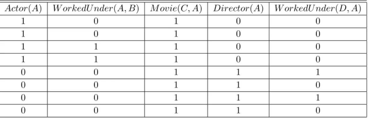
Table 3.3 An example of observations generated
Actor(A) W orkedU nder(A, B) M ovie(C, A) Director(A) W orkedU nder(D, A)
1 0 1 0 0 1 0 1 0 0 1 1 1 0 0 1 1 1 0 0 0 0 1 1 1 0 0 1 1 0 0 0 1 1 1 0 0 1 1 0
be. A greater size of S could help generate more observations. However, generate too many observations may result in an extremely long run time. We set m= 5 to control the number of observations generated.
Table3.3shows the observations we generate for the template node in table3.2. BothA,B
and Dcan take two possible constants, whileC can only beShawshank. So the total number of observations created is 2×2×2 = 8.
3.3 Alternative approach to create template nodes and observations
As we pointed out in section 3.1, some of the template nodes will be filtered out with limited number of free variable in templateN odeArray. We have to setmto limit the number of variable, this is because we generated S which contains all possible assignment of variables in templateN odeArray. Without the restriction of variable number, the size of S could be exponentially large. However, this restriction may also result in loss of some template nodes. Here we present an alternative approach to relax the restriction: we still add these template nodes to thetemplateN odeArray, but create their observations in a different way. The details of the algorithms are listed as follows:
Algorithm 4 displays the details of template nodes construction. The only difference here is that we remove the variable number restriction m, others remain the same. By removing restriction, more template nodes will be introduced, thus more information may be gained.
Algorithm 5 describes the alternative way for generating observations. If a template node only contains the firstmth variables, we use the same way in algorithm3to assign its value in
P: the predicate being considered in this loop
Output:
templateN odeArray: the array contains template nodes
1: Use P to create the head template node, called headNode, and add it to the place 0 of
templateN odeArray.
2: variableN um= number of variables in headN ode
3: for eachGP, ground atom ofP do
4: let CGP be the set of all the true ground atoms that are constant-shared with GP 5: for eachc∈ CGP do
6: newN ode=CreateN ode(c, headN ode, GP)
7: variableN um+ = new variable introduced in newN ode
8: Index=templateN odeArray.f ind(newN ode) 9: if Index <0 then
10: add newN odetotemplateN odeArray
11: else
12: variableN um−= new variable introduced innewN ode
13: end if
14: end for
15: end for
M; otherwise, we make use of an idea in BUSL (Mihalkova and Mooney, 2007), that is, if this node has a true grounding that is constant-shared with the current grounding of headN ode, then its value inM will be set to true. Other things remain the same.
This alternative approach allows more variables to be introduced, thus more template nodes are added to the templateN odeArray, while the size of S remains the same.
3.4 Learn the template and build candidate clauses
Finally, to construct the Markov network template, we need to know how the template nodes are connected by edges. Consider the template nodes as the nodes in the Markov network, and the observation matrix M as the training data, we can find the edges by applying a Markov network structure learning algorithm. Any Markov network structure learning algorithm can be applied here, and we chose the Grow-Shrink Markov Network (GSMN) algorithm by Bromberg et al. (2006). GSMN decides whether two nodes are conditionally independent of each other by using χ2 statistical tests.
Algorithm 5 Generate Observations2
Input:
templateN odeArray : the array of template nodes
m : max free variable number intemplateN odeArray Output:
M : a matrix contains the observations generated
1: letS be the set of all possible assignments to the firstmth variables of the template nodes. 2: foreach si∈ S do
3: append a new array M[i] toM
4: for each nodenj ∈templateN odeArray do 5: if nj only contains firstmth variables then
6: if the ground atom ofnj under the assignment si is truethen 7: M[i][j] =true
8: else
9: M[i][j] =f alse
10: end if
11: else
12: if there exists a true grounding of nj that is constant-shared with the grounding of headN ode then
13: M[i][j] =true 14: else 15: M[i][j] =f alse 16: end if 17: end if 18: end for 19: end for
template, generate all possible clauses from length 1 to the size the of the clique by making disjunctions from the template nodes in the clique, and we try all possible negation/non-negation combinations. Note that we only construct clauses from those template nodes which form cliques in the template; i.e., for any two template nodes in a clause, there must exist an edge between them. Every candidate clause must contain theheadN ode.
Finally, we remove duplicates in the candidates, and evaluate them using the WPLL. Each clause need to be assigned a weight in order to learn the WPLL score. To learn the weight, we useL−BF GSas Richardson and Domingos did (2006). After all the scores are learned, all the candidate clauses are considered for addition to the MLN in order of decreasing score. To speed up the inference and decrease over fitting, we only evaluate candidates with its weight greater thanminW eight. Candidates that do not increase the overall WPLL score are discarded, and the rest are appended to the MLN.
CHAPTER 4. EXPERIMENTAL EVALUATION
4.1 Experimental setup
In this section we describe how we setup our experiment. We implement our algorithm using the Alchemy package available at http:// alchemy.cs.washington.edu.
4.1.1 Datasets
We use a publicly available dataset IMDB database to evaluate our approach. It’s available at http://alchemy.cs.washington.edu. The statistics are shown in Table4.1
Table 4.1 Details of dataset
Dataset Types Constants Predicates True Atoms Total Atoms
IMDB 4 316 10 1540 32615
IMDB.The IMDB dataset is created by Mihalkova and Mooney (2007) from the imdb.com
database, describes a domain about movie. Its predicates describing directors, actors, movies, and their relationships (e.g, Director(person), WorkedUnder(person, person), etc.) It is divided into 5 independent folds. Each fold contains four movies, their directors and actors, etc. We omitted 4 equality predicates (e.g, SamePerson(person, person), SameMovie(movie, movie), etc.) since they are true if and only if their arguments are the same.
4.1.2 Methodology
We compared our algorithms with MSL and BUSL. Both of them are implemented in the Alchemy package. We measured the performance using the metrics used by Kok and Domingos (2005), the area under the precision-recall curve (AUC). AUC is helpful because it displays how good an algorithm predicts the positive atoms in the data, and it is insensitive to a large number
the data as evidence. Exception is the predicates Actor(person) and Director(person), we have to evaluate them together because the groundings of them for the same constant are mutually exclusive, that is, one person can only be either a actor or a director. We set MSL’s parameters as default setting and set BUSL’s parameters as in Mihalkova and Mooney (2007). We set TCSL’sminW eight= 0.5 in our experiments. We performed all runs on the same machine.
4.2 Experimental results
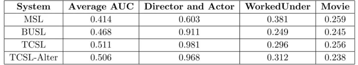
Table4.2reports the average AUCs and the AUCs of three different types of predicates for each algorithm. Higher number of AUC indicates better performance.
Let TCSL be the first algorithm we proposed and TCSL-Alter be the alternative approach to create template nodes and observations. First, we compare our algorithms with MSL and BUSL. Our algorithms’ average AUCs are higher than both MSL and BUSL. For predicate Director(person) and Actor(person), our algorithms significantly outperform MSL, and also improve over BUSL. For predicate WorkedUnder(person, person), our algorithms have higher AUCs than BUSL, but lower than MSL. For predicate Movie(movie, person), all the four al-gorithms’ AUCs are very close. This result suggests that our algorithms outperform BUSL for both types of the predicates, but compare to MSL, our algorithms did worse on the relation-ship predicate WorkedUnder(person, person) and much better on predicating unary predicate. Next we compare TCSL with TCSL-Alter. The average AUCs of TCSL and TCSL-Alter are almost the same. TCSL has a higher AUC for predicate Director(person) and Actor(person), and also slightly better for predicate Movie(movie, person), but performs worse for predicate WorkedUnder(person, person). This result indicates that, since TCSL-Alter introduced more variables and more template nodes than TCSL, that may be the reason it performs better on WorkedUnder(person, person) predicate, but assign the values in M matrix in two different ways may also lead to the decreasing of AUC on Director(person) and Actor(person).
Table4.3 shows the average training time overall for each system. Both TCSL and TCSL-Alter are trained much slower than BUSL and MSL. This is because our algorithms spend most
Table 4.2 Experimental results of AUCs
System Average AUC Director and Actor WorkedUnder Movie
MSL 0.414 0.603 0.381 0.259
BUSL 0.468 0.911 0.249 0.245
TCSL 0.511 0.981 0.296 0.256
TCSL-Alter 0.506 0.968 0.312 0.238
Table 4.3 Experimental running time
System runTimes(min)
MSL 6.91
BUSL 1.42
TCSL 14.67
TCSL-Alter 15.55
of their training time on generating the observations. That’s also the reason that TCSL’s and TCSL-ALter’s run time are very close, although TCSL-Alter introduced more template nodes.
CHAPTER 5. CONCLUSION AND FUTURE WORK
In this paper, we have presented a novel algorithm for the Markov logic network structure learning problem. This approach directly makes use of the data to restrict the search space and guide the construction of candidate clauses, it also generates a set of observations to help construct reliable Markov network templates. Our experiments with a real-world domain have shown the effectiveness of our approach. One bottleneck of this approach is that, it is pretty slow currently because the observation generation algorithm is not very efficient.
Directions for future work includes: improve the efficiency of observation generation process (the significant limitation in our approach); apply our algorithms to larger, richer domains; instead of only consider the ground atoms that is constant-shared with headN ode, introduce multiple hops (e.g., variabilize the ground atoms which are constant-shared with template nodes already obtained) of template nodes in the template nodes construction part .
REFERENCES
[1] Getoor, L., and Taskar, B. (Eds.). (2007).Introduction to statistical relational learning.
[2] Richardson, M., and Domingos, P. (2006). Markov logic networks.Machine Learning 62(1-2): 107-136.
[3] Kok, S., and Domingos, P. (2005). Learning the structure of Markov logic networks. In
Proceedings of the 22 International Conference on Machine Learning,441-448. ACM. [4] Richards, B. L., and Mooney, R. J. (1992). Learning relations by pathfinding. 10th Nat.
Conf. On Art. Intel.50-55
[5] Pearl, J. (1988). Probabilistic reasoning in intelligent systems: Networks of plausible
in-ference.San Francisco, CA: Morgan Kaufmann.
[6] Genesereth, M. R., and Nilsson, N. J. (1987).Logical foundations of artificial intelligence.
San Mateo, CA: Morgan Kaufmann.
[7] Bromberg, F., Margaritis, D., and Honavar, V. (2006). Efficient Markov network structure discovery using independence tests.SDM-06
[8] Mihalkova, L., and Mooney, R. J. (2007). Bottom-up learning of Markov logic network structure.24th Int. Conf. on Mach. Learn. (pp. 339-352)
[9] Liu, D. C., and Nocedal, J. (1989). On the limited memory BFGS method for large scale optimization.Mathematical Programming, 45, 503528.