On Nonnegative Matrix Factorization Algorithms for Signal-Dependent Noise with Application to Electromyography Data

On Nonnegative Matrix Factorization Algorithms

for Signal-Dependent Noise with Application

to Electromyography Data

Karthik Devarajan [email protected]

Department of Biostatistics and Bioinformatics, Fox Chase Cancer Center, Philadelphia, PA 19111, U.S.A.

Vincent C. K. Cheung [email protected]

Department of Brain and Cognitive Sciences and McGovern Institute for Brain Research, MIT, Cambridge, MA 02139, U.S.A.

Nonnegative matrix factorization (NMF) by the multiplicative updates algorithm is a powerful machine learning method for decomposing a high-dimensional nonnegative matrixVinto two nonnegative matrices, WandH, whereV ∼W H. It has been successfully applied in the analysis and interpretation of large-scale data arising in neuroscience, computa-tional biology, and natural language processing, among other areas. A distinctive feature of NMF is its nonnegativity constraints that allow only additive linear combinations of the data, thus enabling it to learn parts that have distinct physical representations in reality. In this letter, we de-scribe an information-theoretic approach to NMF for signal-dependent noise based on the generalized inverse gaussian model. Specifically, we propose three novel algorithms in this setting, each based on multiplica-tive updates, and prove monotonicity of updates using the EM algorithm. In addition, we develop algorithm-specific measures to evaluate their goodness of fit on data. Our methods are demonstrated using experimen-tal data from electromyography studies, as well as simulated data in the extraction of muscle synergies, and compared with existing algorithms for signal-dependent noise.

1 Introduction

Nonnegative matrix factorization (NMF) was introduced as an unsuper-vised, parts-based learning paradigm, in which a high-dimensional

non-negative matrixVis decomposed into two matrices,WandH, each with

nonnegative entries,V ∼WH, by a multiplicative updates algorithm (Lee &

Seung, 1999, 2001). In the past decade, NMF has been increasingly applied in a variety of areas involving large-scale data. These include neuroscience,

Neural Computation26, 1128–1168(2014) c 2014 Massachusetts Institute of Technology

computational biology, natural language processing, information retrieval, biomedical signal processing and image analysis. (For a review of its appli-cations, see Devarajan, 2008.)

Lee and Seung (2001) outlined algorithms for NMF based on the gaussian and Poisson likelihoods. Since their seminal work, numerous variants, ex-tensions, and generalizations of the original NMF algorithm have been pro-posed in the literature. For example, Hoyer (2004), Shahnaz, Berry, Pauca, and Plemmons (2006), Pascual-Montano, Carazo, Kochi, Lehmann, and Pascual-Marqui (2006), and Berry, Browne, Langville, Pauca, and Plemmons (2007) extended NMF to include sparseness constraints. Wang, Kossenkov, and Ochs (2006) introduced LS-NMF that incorporated variability in the data. Cheung and Tresch (2005) and Devarajan and Cheung (2012) extended the NMF algorithm to include members of the exponential family of distri-butions while Devarajan and Ebrahimi (2005, 2008), Devarajan (2006), and Devarajan, Wang, and Ebrahimi (2011) formulated a generalized approach to NMF based on the Poisson likelihood that included various well-known distance measures as special cases. Dhillon and Sra (2005) and Kompass (2007) have also proposed generalized divergence measures for NMF. chocki, Zdunek, and Amari (2006), Cichocki, Lee, Kim, and Choi (2008), Ci-chocki, Zdunek, Phan, and Amari (2009), and CiCi-chocki, Cruces, and Amari (2011) extensively developed a series of generalized algorithms for NMF

based onα- andβ-divergences while F´evotte and Idier (2011) recently

ex-tended it by proposing some novel algorithms. The work of Cichocki et al. (2009) provides a detailed reference on this subject.

The main focus of this letter is on NMF algorithms for signal-dependent noise with particular emphasis on the generalized inverse gaussian family of distributions. This family includes the well-known gamma model for signal-dependent noise as a special case. It also includes the inverse gaus-sian model as a special case, among others. Each model incorporates signal dependence in noise in structurally different ways based on the mean-variance relationship, as evidenced in the following sections. These models are embedded within the framework of the exponential family of models outlined in Cheung and Tresch (2005) and can be obtained as special cases of

β-divergence proposed in Cichocki et al. (2006, 2009). In each case, the NMF

algorithm is based on maximizing the likelihood or, equivalently, minimiz-ing a cost function defined by the Kullback-Leibler divergence between the

input matrixVand the reconstructed matrixWH.

We describe an approach to NMF for signal-dependent noise by extend-ing the standard likelihood approach to include two well-known alterna-tive cost functions from information theory for quantifying this divergence:

the dual Kullback-Leibler divergence and theJ-divergence. Based on these

measures, we propose three NMF algorithms applicable when the data ex-hibit signal-dependent noise. For each algorithm, we provide a rigorous proof of monotonicity of updates using the EM algorithm. We describe a principled method for selecting the appropriate rank of the factorization and

develop algorithm-specific measures to quantify the variation explained by the chosen model. We demonstrate the applicability of our methods using experimental data from electromyography (EMG) studies, as well as sim-ulated data in extracting muscle synergies, and compare the performance of our proposed methods with existing algorithms for signal-dependent noise.

The remainder of the letter is organized as follows. Section 2 provides the necessary background required for the information-theoretic approach we describe. It is intended to serve as a brief tutorial on fundamental concepts, terminology, basic quantities of interest for our problem, and their interpre-tations. Section 3 provides a detailed overview of existing NMF algorithms for signal-dependent noise and places them within the broader context of NMF algorithms based on generalized divergence measures. Furthermore, it describes our proposed NMF algorithms for signal-dependent noise and provides multiplicative update rules. Section 4 outlines methods for model selection and evaluation, while section 5 presents an application of our methods to EMG data and a comparison to existing methods. Section 6 provides a summary and conclusions. Detailed proofs of monotonicity of updates for the proposed algorithms are relegated to the appendix.

2 Background and Preliminaries

2.1 Directed Divergence and Divergence. Suppose we are interested

in testing a set of hypotheses denoted byH_i,i=0,1 that a random variable

X is from populationiwith probability measureμ_i Assume thatμ₀ and

μ1are absolutely continuous with respect to each other and thatXtakes

values on the entire real line. LetP(H_i)denote the prior probabilities, f,g

the density functions, andF,Gthe distribution functions corresponding to

the hypothesisH_i,i=0,1, respectively. IfP(H_i|x)denotes the conditional

(or posterior) probability ofH_igivenX=x, then, using Bayes’ theorem, we

have P(H₀|x)= P(H0)f(x) P(H₀)f(x)+P(H₁)g(x) and P(H₁|x)= P(H1)g(x) P(H₀)f(x)+P(H₁)g(x). Hence, log f(x) g(x) =log P(H₀|x) P(H₁|x) −log P(H₀) P(H₁) ,

that is, the logarithm of the likelihood ratio, defined as the negative

differ-ence between the logarithm of the odds in favor ofH₀before and after the

observationX=x, is the information inX=xfor discrimination in favor

ofH₀againstH₁(Kullback, 1959).

Suppose thatxis not given and there is not specific information on the

whereabouts ofxother thanx∈S. The mean information per observation,

averaged over all the valuesxofX, for discrimination in favor ofH₀against

H₁is thus I(f,g)= f(x)log P(H₀|x) P(H₁|x) dx−log P(H₀) P(H₁) = f(x)log f(x) g(x) dx. (2.1)

This quantity is known as Kullback-Leibler divergence betweenfandg,

the negative log likelihood or empirical entropy. Similarly, the measure

I(g,f) is defined as the mean information per observation, averaged over

all the valuesxofX, for discrimination in favor ofH₁ againstH₀ and is

given by I(g,f)= g(x)log P(H₁|x) P(H₀|x) dx−log P(H₁) P(H₀) = g(x)log g(x) f(x) dx. (2.2)

This quantity is known as the dual Kullback-Leibler divergence betweenf

andgor the negative empirical log likelihood. In light of these definitions,

I(f,g) andI(g,f) are also referred to as directed divergences. These quantities

are nonnegative definite and are zero if and only if f(x)=g(x) almost

everywhere (Kullback, 1959; Owen, 2001).

Using directed divergencesI(f,g) andI(g,f), one can define J-divergence

J(f,g) as J(f,g)=I(f,g)+I(g,f) = (f(x)−g(x))log f(x) g(x) dx, (2.3)

which is a measure of the divergence or the difficulty of discriminating

between the hypothesesH₀andH₁. A key feature ofJ(f,g) is symmetry with

respect to the measuresμ₀ andμ₁. It has all the properties of a distance

measure (metric) except the triangle inequality, is nonnegative definite, and

2.2 Motivating NMF for Signal-Dependent Noise

2.2.1 The Generalized Inverse Gaussian Distribution. A nonnegative

ran-dom variableXis said to be a member of the family of generalized inverse

gaussian (GIG) distributions if its probability density function is given by f(x)=γ δ ξ 1 2K_ξ(δγ )x ξ−1_e−1 2(δ2x−1+γ2x), x>0, (2.4)

whereγ >0,δ >0,ξ ∈ , and,K_ξis the modified Bessel function of the third

kind with indexξ. In the limiting caseδ→0 whenξ >0, f(x)reduces to a

gamma distribution with density g(x)= β

α

(α)xα−1e−βx, x>0, (2.5)

whereα=ξ >0 andβ= γ₂2 >0. The mean-variance relationship can be

written as Var(X)= α β2 = 1 α[E(X)] 2 (2.6) and thus indicates a quadratic dependence of variance on the mean. When

ξ = −1

2, f(x)reduces to an inverse gaussian distribution with density

h(x)= λ 2πx3 1/2 exp −λ(x−μ) 2 2μ2_x , (2.7) whereλ=δ2_andμ= δ

γ. The mean-variance relationship can be written as

Var(X)= μ

3

λ =

[E(X)]3

λ (2.8)

and thus indicates a cubic dependence of variance on the mean.

Other special cases of the GIG family of distributions include the inverse gamma and hyperbolic distributions (Eberlein & Hammerstein, 2004). In this letter, we focus on the gamma and inverse gaussian distributions as data-generating models for signal-dependent noise in the context of NMF.

2.2.2 Divergence Measures for Signal-Dependent Noise. The discrimination

information functions defined above were introduced by Kullback and Leibler (1951) and serve as divergence measures for comparing two

g(x)in equations 2.1 to 2.3 based on the gaussian (normal), gamma or in-verse gaussian models, one can obtain various divergence measures for NMF based on the empirical entropy, empirical likelihood, or a

combina-tion of these. Throughout the presentacombina-tion, we useKL,KLd_{, andJto denote}

Kullback-Leibler, dual Kullback-Leibler, andJ-divergence, respectively. In

each case, the subscriptsN,G, andIG are used to refer to the gaussian,

gamma, and inverse gaussian models, respectively. The termKL divergence

has been used in the literature to refer to that based on the Poisson model.

However, it is important to note that the termsKL, dualKL, andJ-divergence

used in this letter refer to generic divergence measures between any two

densitiesfandgas defined in equations 2.1 to 2.3 and are not model specific.

Each divergence measure can be defined specifically for a particular choice of model, as outlined below.

For two normal random variables with means μ₁ and μ₂ (and equal

varianceσ2_{) and corresponding probability density functions f(x)andg(x),}

it can be shown that

KL_N(f,g)=KLd_N(f,g)= 1

2J=

1

2σ2(μ1−μ2)2. (2.9)

Using equation 2.5, it can be shown that for two gamma random variables

with meansμ₁andμ₂(and common shape parameterα) and corresponding

probability density functions f(x)andg(x),

KL_G(f,g)=α μ1 μ2 −log μ1 μ2 −1 , (2.10) KLd_G(f,g)=α μ2 μ1 −log μ2 μ1 −1 (2.11) and J_G(f,g)=α (μ1−μ2)2 μ1μ2 . (2.12)

Similarly, using equation 2.7, it can be shown that for two inverse gaussian

random variables with meansμ₁andμ₂(and common shape parameterλ)

and corresponding probability density functions f(x)andg(x),

KL_IG(f,g)=λ(μ1−μ2) 2 2μ₁μ2 2 (2.13) and KLd_IG(f,g)=λ(μ1−μ2) 2 2μ2 1μ2 . (2.14)

It will become clear in section 3 that none of the parameter coefficients in the divergence equations 2.9 to 2.14 play any role in the derivation of the NMF

algorithms. Hence, we assume that 2σ2_{=α=λ/2=1 without loss of}

gen-erality. It should be noted that this assumption is consistent with the basic formulation in NMF and that numerous other divergence measures avail-able in the literature for NMF implicitly make such assumptions (Cichocki et al., 2006, 2008, 2009; F´evotte & Idier, 2011; Kompass, 2007; Devarajan & Cheung, 2012).

We motivate nonnegative matrix factorizations in the context of dimen-sion reduction of high-dimendimen-sional electromyography (EMG) data. EMG data are typically presented as a matrix in which the rows correspond to different muscles, the columns to disjoint, sequentially sampled time intervals, and each entry to the EMG signal of a given muscle in a given

time interval. In EMG studies, the number of muscles,p, is typically, fewer

than fifty; the number of time intervals,n, is typically in the tens of

thou-sands; and the matrix of EMG signal intensitiesVis of size p×nso that

each column ofVrepresents an activation vector in the muscle space at one

time instance. Our goal is to find a small number of muscle synergies, each defined as a nonnegative, time-invariant activation balance profile in the

p-dimensional muscle space. This is accomplished with a decomposition of

the matrixVinto two matrices with nonnegative entries,V∼WH, where

Whas a sizep×r, so that each column is a time-invariant muscle synergy in

thep-dimensional muscle space and the matrixHhas sizer×n, so that each

column contains the activation coefficients for thersynergies inWfor one

time instance. The number of synergiesris chosen so that(n+p)r<np.

The entry h_ai of H is the coefficient of time interval i in synergy a,

and the entry w_ja of W is the expression level of synergya in muscle j,

wherea=1,2, . . . ,r.

The first step in obtaining an approximate factorization forVis to define

cost functions that measure the divergence between the observed matrixV

and the product of the factored matricesWH. We can express this in the

form of a linear model as

V =WH+, (2.15)

whererepresents noise. NMF algorithms for signal-dependent noise based

onKLdivergence (see equations 2.10 and 2.13, respectively) for gamma and

inverse gaussian models exist in the literature (Cheung & Tresch, 2005; Cichocki et al, 2009; F´evotte & Idier, 2011). In this letter, we propose three novel NMF algorithms for handling signal-dependent noise, specifically

based on dualKLandJ-divergence for gamma and inverse gaussian models

(see equations 2.11, 2.12, and 2.14). The appropriate cost function for each

model is obtained by simply substitutingμ₁andμ₂in equations 2.9 to 2.14

2.2.3 Application of NMF to EMG Data. We present an application in-volving the analysis of EMG data, electrical signals recorded from muscles that reflect how they are activated by the nervous system for a particular posture or movement. It is well known in the literature that EMG data exhibit signal-dependent noise (Harris & Wolpert, 1998; Cheung, d’Avella, Tresch, & Bizzi, 2005). One long-standing question in neuroscience con-cerns how the motor system coordinates the activations of hundreds of skeletal muscles, representing hundreds of degrees of freedom to be con-trolled (Bernstein, 1967). They define an immense volume of possible motor commands that the central nervous system (CNS) must search through for the execution of even an apparently simple movement. It has been argued that the CNS simplifies the complexity of movement and postural control arising from high dimensionality by activating groups of muscles as indi-vidual units, known as muscle synergies (Tresch, Saltiel, d’Avella, & Bizzi, 2002; Giszter, Patil, & Hart, 2007; Bizzi, Cheung, d’Avella, Saltiel, & Tresch, 2008; Ting, Chvatal, Safavynia, & McKay, 2012). As modules of motor con-trol, muscle synergies serve to reduce the search space of motor commands, reduce potential redundancy of motor commands for a given movement, and facilitate learning of new motor skills (Poggio & Bizzi, 2004). Numerous laboratories have utilized linear factorization algorithms to extract muscle synergies from multichannel EMGs recorded from humans and animals (reviewed in Bizzi & Cheung, 2013). In particular, several studies have demonstrated that the muscle synergies returned by the gaussian NMF could be neurophysiological entities utilized by the CNS for the production of natural motor behaviors (Saltiel, Wyler-Duda, d’Avella, Tresch, & Bizzi, 2001; Tresch, Cheung, & d’Avella, 2006; Overduin, d’Avella, Carmena, & Bizzi, 2012).

It has been further posited that muscle synergies for locomotion are basic units of the so-called central pattern generators (CPGs) whose or-ganizations are independent of the pattern of sensory feedback. Cheung et al. (2005) sought to demonstrate this possibility by recording hind-limb EMGs from bullfrogs during jumping and swimming, before and after deafferentation or the surgical procedure of eliminating sensory in-flow into the spinal cord by cutting the dorsal nerve roots. By apply-ing a manipulated version of the gaussian NMF to the data matrix that pooled the intact and deafferented EMGs together, they found three to six, out of four to six, muscle synergies were preserved after deafferenta-tion. The preserved synergies were then interpreted as basic components of the CPGs. Here, we ask whether the NMF algorithms based on gamma or inverse gaussian noise can better identify CPG components by dis-covering more muscle synergies shared between the pre- and postdeaf-ferentation data sets than the traditional gaussian NMF. We hypothesize that the NMF algorithms derived from signal-dependent noise outperform the gaussian NMF in their ability to discover shared muscle synergies, be-cause signal-dependent noise formulations should better model the noise

properties of EMG signals than a gaussian formulation (Harris & Wolpert, 1998).

The data analyzed here were previously described in Cheung et al. (2005). EMGs during unrestrained jumping and swimming were collected from

four adult bullfrogs (Rana catesbeiana) before and after a complete hind limb

deafferentation was achieved by severing dorsal roots 7 to 9. Intramuscu-lar EMG electrodes were surgically implanted into the following muscles in the right hind limb: rectus internus major (RI), adductor magnus (AD), semimembranosus (SM), semitendinosus (ST), iliopsoas (IP), vastus inter-nus (VI), rectus femoris anticus (RA), gastrocnemius (GA), tibialis anticus (TA), peroneus (PE), biceps (BI), sartorius (SA), and vastus externus (VE). The collected EMG signals were amplified (gain of 10,000) and bandpass-filtered (10–1000 Hz) through differential alternating-current amplifiers, then digitized at 1000 Hz. Using custom software written in Matlab (R2010b; Math-Works, Natick, MA), the EMG signals were further high-pass-filtered with a window-based finite impulse response (FIR) filter (50th order; cutoff of 50 Hz) to remove any motion artifacts, then rectified, low-pass-filtered (FIR; 50th order; 20 Hz), and finally integrated over 10 ms intervals. The preprocessed data of each muscle were then normalized to the maximum EMG value of that muscle attained in the entire experiment.

The EMG signal is a spatiotemporal summation of the motor action po-tentials traveling along the muscle fibers of the thousands of motor units in the recorded muscle. The high-frequency components of the EMG reflect, in addition to noise, the contribution of these action potentials. In motor neuroscience, it is customary to perform low-pass filtering on the recorded EMGs to obtain an “envelope” of muscle activation, which should reflect the higher-level control signals originating from the brain and spinal cord that specify the degree of muscle contraction for generating the desired force (with the force magnitude dictated by the muscle’s length and force-velocity relationships). Since we are interested in discovering structures at the level of control signals for muscular contraction (i.e., muscle synergies) and since signal dependent noise is thought to occur at this control-signal level, it is appropriate to apply NMF to filtered EMG data. There is a siz-able literature on using the gaussian NMF algorithm for extracting muscle synergies from filtered EMG data (reviewed in Bizzi & Cheung, 2013). Moreover, filtering the EMGs before NMF extraction would allow an easier comparison of our results with those in the literature.

One approach to visualizing signal dependence in these data is to plot the variability as a function of the mean for EMG signals from each muscle separately. Any observed trend in the mean-variance relationship would in-dicate some form of signal dependence, the exact nature of the relationship being dependent on the data-generating mechanism. For each muscle, the mean and variance of the EMG signal were computed for moving windows across time. Several window sizes ranging from 3 to 50 were explored, and it was observed that mean-variance relationship was not sensitive to the

choice of window size. Our choice of window size was based on a physio-logical justification. There has been an earlier result suggesting that bursts with 275 msec duration could be a fundamental pulse unit in the frog spinal cord (Hart & Giszter, 2004). Since our integration time interval is 10 ms, we used a window size of 28 so that each window corresponded to the duration of this fundamental drive.

Using equation 2.6, we can rewrite the mean-variance relationship for a

gamma model in terms of the standard deviationσ (X)as

σ (X)=Var(X)= √1

αE(X).

Taking the logarithm on both sides, we obtain

logσ (X)=logE(X)−1

2logα.

Figure 1A shows a plot of the logarithm of the estimated standard de-viation against the logarithm of the estimated mean for moving windows across time for the intact jump of one frog for the muscle TA. The black solid line represents a linear fit to the data. The proximity of the estimated slope of this line to unity provides strong evidence that a gamma model adequately represents the mean-variance relationship in these data. The logarithmic transformation provides variance stabilization and aids in interpreting the slope of the fit. Panels A to D in Figure 1 display such plots for each of the four behaviors of selected muscles and frogs. At the top of each panel in this figure, the estimate of the slope and goodness-of-fit measures such as the

root mean squared error (RSE) and adjustedR2_{are listed along with frog}

behavior and name of muscle. This figure is representative of the mean-variance relationship typically observed in our frog EMG data. Table 1 lists

the estimates of slope and adjustedR2_{(mean±SD forN=4 frogs) from}

the least squares fit for each behavior and muscle. It is evident from these results that the gamma model provides an overall good fit of the EMG data. In the following section, we discuss NMF algorithms for signal-dependent noise. We begin with a survey of existing work in this area before describing three novel algorithms for this problem. A detailed anal-ysis of the data sets described here, including a comparison of existing approaches to our proposed methods, is presented in section 5.

3 NMF Algorithms for Signal-Dependent Noise

3.1 Existing Work. Cheung and Tresch (2005) proposed a heuristic NMF algorithm for the exponential family of distributions that embeds the gaus-sian, Poisson, gamma, and inverse gaussian models. They provided

Figure 1: Illustration of the mean-variance relationship for the frog EMG data. Plot of the logarithm of the estimated standard deviation against the logarithm of the estimated mean for moving windows across time for each behavior of selected muscles and frogs. Each panel displays the mean-variance relationship for a particular behavior. (A) Intact jump. (B) deafferented jump. (C) intact swim. (D) deafferented swim. In each panel, the black solid line represents a linear fit to the data and estimates of the slope, root mean squared error (RSE), and adjustedR2_{are listed at the top of each panel.}

size in the gradient based on the negative log likelihood (or, equivalently,

KLdivergence). In independent work, Cichocki et al. (2006) also proposed

a similar heuristic algorithm based on the generalizedβ-divergence and

provided multiplicative update rules forWandH.β-divergence between

the input matrixVand reconstructed matrixWHis given by

D_β(V,WH)= 1 β(β−1) i,j V_{i j}β−βV_{i j}(WH)β−1_{i j} +(β−1)(WH)β_{i j} , β∈ \{0,1}. (3.1)

β-divergence includes the gaussian (β =2), Poisson (β→1), gamma

T able 1: Empirical Assessment of Mean-V ariance Relationship: Estimated Slope ( ˆ_β)and Adjusted R 2fr om Least Squar es Fit of Standar d Deviation versus Mean (Log Scale) (Mean ± SD for N = 4 Fr ogs). Measur e of F it Behavior IP VI RA GA RI ˆ_β Intact jump 1.03 ± 0.09 1.25 ± 0.09 1.21 ± 0.09 1.21 ± 0.05 1.82 ± 0.11 Deaf fer ented jump 1.02 ± 0.04 1.18 ± 0.10 1.13 ± 0.07 1.23 ± 0.04 1.52 ± 0.09 Intact swim 1.09 ± 0.06 1.32 ± 0.12 1.13 ± 0.06 1.21 ± 0.14 2.37 ± 0.91 Deaf fer ented swim 1.12 ± 0.12 1.30 ± 0.15 1.11 ± 0.14 1.21 ± 0.08 2.38 ± 0.63 Adjusted R 2 Intact jump 0.92 ± 0.04 0.94 ± 0.05 0.92 ± 0.02 0.94 ± 0.02 0.85 ± 0.02 Deaf fer ented jump 0.88 ± 0.02 0.92 ± 0.03 0.91 ± 0.02 0.94 ± 0.01 0.90 ± 0.15 Intact swim 0.82 ± 0.03 0.90 ± 0.02 0.87 ± 0.05 0.90 ± 0.06 0.74 ± 0.11 Deaf fer ented swim 0.84 ± 0.03 0.88 ± 0.04 0.85 ± 0.04 0.90 ± 0.03 0.78 ± 0.06 AD SM ST T A PE ˆ_β Intact jump 1.35 ± 0.08 1.32 ± 0.08 0.90 ± 0.05 1.04 ± 0.04 1.16 ± 0.09 Deaf fer ented jump 1.31 ± 0.12 1.27 ± 0.04 0.90 ± 0.05 0.94 ± 0.07 1.08 ± 0.12 Intact swim 1.52 ± 0.11 1.50 ± 0.10 1.16 ± 0.10 1.04 ± 0.05 1.02 ± 0.09 Deaf fer ented swim 1.48 ± 0.29 1.56 ± 0.22 1.33 ± 0.16 1.09 ± 0.13 1.03 ± 0.13 Adjusted R 2 Intact jump 0.93 ± 0.01 0.91 ± 0.03 0.82 ± 0.08 0.90 ± 0.03 0.92 ± 0.04 Deaf fer ented jump 0.92 ± 0.01 0.90 ± 0.02 0.76 ± 0.08 0.86 ± 0.03 0.89 ± 0.05 Intact swim 0.89 ± 0.02 0.90 ± 0.01 0.86 ± 0.01 0.80 ± 0.05 0.82 ± 0.05 Deaf fer ented swim 0.88 ± 0.03 0.90 ± 0.03 0.88 ± 0.03 0.88 ± 0.09 0.81 ± 0.06 BI SA VE ˆ_β Intact jump 1.03 ± 0.03 1.17 ± 0.08 1.34 ± 0.12 Deaf fer ented jump 1.03 ± 0.06 1.06 ± 0.03 1.17 ± 0.04 Intact swim 1.15 ± 0.05 1.24 ± 0.18 1.31 ± 0.17 Deaf fer ented swim 1.19 ± 0.10 1.34 ± 0.15 1.21 ± 0.18 Adjusted R 2 Intact jump 0.88 ± 0.04 0.88 ± 0.04 0.92 ± 0.02 Deaf fer ented jump 0.89 ± 0.02 0.88 ± 0.03 0.90 ± 0.03 Intact swim 0.86 ± 0.03 0.86 ± 0.03 0.88 ± 0.04 Deaf fer ented swim 0.88 ± 0.04 0.86 ± 0.06 0.86 ± 0.04

be noted that this generalized divergence is related to the other divergence measures independently described in the literature (such as those in Kom-pass, 2007; Cichocki et al., 2008; Devarajan et al., 2011; and Devarajan & Ebrahimi, 2005) via transformations. For NMF algorithms based on gamma and inverse gaussian models stemming from the work of Cheung and Tresch (2005) and Cichocki et al. (2006), monotonicity of updates cannot be established, and they remain heuristic. Recently, however, F´evotte and Idier (2011) proposed a rigorous majorization-maximization (MM)

algo-rithm based onβ-divergence that enables monotonicity of updates forW

andHto be theoretically established. Moreover, they provided generalized

multiplicative update rules forWandHthat were seen to be different from

heuristic updates. We refer to these as the heuristic and MM algorithms for gamma and inverse gaussian models. In each algorithm, it is straightfor-ward to see that the divergence measure for gamma and inverse gaussian

models is that based onKLdivergence. For the NMF problemV∼WH,

when we used equation 2.10 the kernel ofKLdivergence for the gamma

model can be written as

KL_G(V,WH)= i,j −log Vi j (WH)_{i j} + Vi j (WH)_{i j}−1 . (3.2)

This is commonly referred to as the Itakuro-Saito divergence (Cichocki et al.,

2009; F´evotte & Idier, 2011). Heuristic updates forWandHare given by

Ht+1 a j =Ha jt ⎛ ⎜ ⎜ ⎝ i V_{i j} (bWibHb jt) 2Wia i 1 bWibHb jt W_ia ⎞ ⎟ ⎟ ⎠, (3.3) W_iat+1=W_iat ⎛ ⎜ ⎜ ⎝ j V_{i j} (bWibtHb j) 2Ha j j 1 bW t ibHb j H_{a j} ⎞ ⎟ ⎟ ⎠, (3.4)

and MM updates are given by

Ht_{a j}+1=H_{a j}t ⎛ ⎜ ⎜ ⎝ i V_{i j} (bWibH t b j) 2Wia i 1 bWibHtb j W_ia ⎞ ⎟ ⎟ ⎠ 1/2 , (3.5) W_iat+1=W_iat ⎛ ⎜ ⎜ ⎝ j V_{i j} (bW t ibHb j) 2Ha j j 1 bW t ibHb j H_{a j} ⎞ ⎟ ⎟ ⎠ 1/2 . (3.6)

Similarly, when we use equation 2.13, the kernel ofKLdivergence for the inverse gaussian model can be written as

KL_IG(V,WH)=

i,j

{V_{i j}−(WH)_{i j}}2

V_{i j}(WH)_{i j}2 . (3.7)

Heuristic updates forWandHare given by

H_{a j}t+1=H_{a j}t ⎛ ⎜ ⎜ ⎜ ⎝ i V_{i j} (_bW_ibHt b j) 3W_ia i 1 bWibHtb j 2 W_ia ⎞ ⎟ ⎟ ⎟ ⎠, (3.8) W_iat+1=W_iat ⎛ ⎜ ⎜ ⎜ ⎝ j V_{i j} (_bWt ibHb j) 3H_{a j} j 1 bWibtHb j 2 H_{a j} ⎞ ⎟ ⎟ ⎟ ⎠, (3.9)

and MM updates are given by

H_{a j}t+1=H_{a j}t ⎛ ⎜ ⎜ ⎜ ⎝ i V_{i j} (_bW_ibHt b j) 3W_ia i 1 bWibHb jt 2 W_ia ⎞ ⎟ ⎟ ⎟ ⎠ 1/3 , (3.10) W_iat+1=W_iat ⎛ ⎜ ⎜ ⎜ ⎝ j V_{i j} (_bWt ibHb j) 3H_{a j} j 1 bWibtHb j 2 H_{a j} ⎞ ⎟ ⎟ ⎟ ⎠ 1/3 . (3.11)

Using results from Cheung and Tresch (2005), Cichocki et al. (2006), and F´evotte and Idier (2011), it is straightforward to obtain the above up-date rules in each specific case. For consistency, we use the notation KLH

G,KLMMG ,KLHIG, andKLMMIG to represent the heuristic and MM algorithms

for gamma and inverse gaussian models, respectively.

3.2 Proposed Algorithms. In this section, we propose two novel NMF

algorithms based on dual KL divergence, one each for the gamma and

inverse gaussian models, and one algorithm based on J-divergence for

the gamma model. We use the notation KLd

G,KLdIG, and JG, respectively,

multiplicative update rules forWandHare provided for each, while proofs of monotonicity of updates are detailed in the appendix.

3.2.1 Gamma Model: Algorithm Based on Dual KL Divergence. Using

equation 2.11, the kernel of dualKLdivergence for the gamma model can

be written as KLd_G(V,WH)= i,j log Vi j (WH)_{i j} +(WH)i j V_{i j} −1 . (3.12)

Theorem 1. The divergence K Ld

G(V,WH)in equation 3.12 is nonincreasing

under the multiplicative update rules for W and H given by equations 3.13 and 3.14. It is also invariant under these updates if and only if W and H are at a stationary point of the divergence.

Proof. See the appendix.

Update rules forHandWare

Ht+1 a j =Ha jt ⎛ ⎜ ⎜ ⎝ i 1 bWibH t b j W_ia i W_ia V_{i j} ⎞ ⎟ ⎟ ⎠, (3.13) W_iat+1=W_iat ⎛ ⎜ ⎜ ⎝ j 1 bWibtHb j H_{a j} j H_{a j} V_{i j} ⎞ ⎟ ⎟ ⎠. (3.14)

3.2.2 Gamma Model: Algorithm Based on J Divergence. When equation 2.12

is used, the kernel ofJdivergence for the gamma model can be written as

J_G(V,WH)= i,j (WH)_{i j} V_{i j} + V_{i j} (WH)_{i j} −2 = i,j (V_{i j}−(WH)_{i j})2 V_{i j}(WH)_{i j} . (3.15)

Theorem 2. The divergence J_G(V,WH)defined in equation 3.15 is nonincreas-ing under the multiplicative update rules for W and H given by equations 3.16 and 3.17. It is also invariant under these updates if and only if W and H are at a stationary point of the divergence.

Update rules forHandWare H_{a j}t+1=H_{a j}t ⎛ ⎜ ⎜ ⎜ ⎝ i V_{i j} bWibHtb j 2 W_ia V_{i j} i W_ia V_{i j} ⎞ ⎟ ⎟ ⎟ ⎠ 1/2 , (3.16) W_iat+1=W_iat ⎛ ⎜ ⎜ ⎜ ⎝ j V_{i j} bWibtHb j 2 H_{a j} V_{i j} j H_{a j} V_{i j} ⎞ ⎟ ⎟ ⎟ ⎠ 1/2 . (3.17)

3.2.3 Inverse Gaussian Model: Algorithm Based on Dual KL Divergence.

When equation 2.14 is used, the kernel of dualKLdivergence for the inverse

gaussian model can be written as

KLd_IGV,WH= i,j V_{i j}−(WH)_{i j}2 V2 i j(WH)_{i j} . (3.18)

Theorem 3. The divergence K Ld

I G(V,WH)defined in equation 3.18 is

nonin-creasing under the multiplicative update rules for W and H given by equations 3.19 and 3.20. It is also invariant under these updates if and only if W and H are at a stationary point of the divergence.

Proof. See the appendix.

Update rules forHandWare

H_{a j}t+1=H_{a j}t ⎛ ⎜ ⎜ ⎜ ⎝ i V_{i j} bWibHtb j 2 W_ia V_{i j}2 i W_ia V_{i j}2 ⎞ ⎟ ⎟ ⎟ ⎠ 1/2 , (3.19) W_iat+1=W_iat ⎛ ⎜ ⎜ ⎜ ⎝ j V_{i j} bWibtHb j 2 H_{a j} V_{i j}2 j H_{a j} V_{i j}2 ⎞ ⎟ ⎟ ⎟ ⎠ 1/2 . (3.20)

When equations 2.13 and 2.14 are used, J-divergence for the inverse

gaussian model can be written in terms of V and WH. However, we

EM approach, and the monotonicity of updates cannot be theoretically established.

Remark. The divergences 3.12, 3.15, and 3.18 and their corresponding

update rules forWandH(equations 3.13 and 3.14, 3.16 and 3.17, and 3.19

and 3.20, respectively) containV_ij in the denominator of various terms.

Theoretically, this should not cause any numerical issues (such as division

by zero) sinceV_{i j}>0 for both gamma and inverse gaussian models (i.e.,

zero is not in their domain). However, in a practical setting, due to data preprocessing, a few zero entries may sometimes occur in the input matrix

V. In such cases, it is reasonable to set the zero entries to the smallest nonzero

entry inV.

4 Model Selection and Measuring Goodness of Fit

Starting with random initial values forWandH, the multiplicative update

rules for any given NMF algorithm outlined in section 3 ensure monotonic-ity of updates for that run; however, the algorithm may not necessarily converge to the same solution on each run. In general, NMF algorithms are prone to this problem of local minima. For a given NMF algorithm and a

prespecified rankrfactorization, the corresponding divergence (or

recon-struction error) computed at the final converged values ofWandHfor a set

of random initial values can be used directly in model selection and to mea-sure goodness of fit. One solution is to use the factorization from the run that results in the best reconstruction (quantified by minimum reconstruction error across multiple runs) for evaluation using different quantities. Below, we define two quantities of interest for this purpose based on

algorithm-specific minimum reconstruction errorE.

4.1 Proportion of Explained Variation. We propose several new mea-sures to quantify the variation explained by the various algorithms for signal-dependent noise discussed in this letter. For each prespecified rank

r, the proportion of explained variation (or empirical uncertainty),R2_{, is}

dependent on the particular algorithm and model used in the factorization.

For the gaussian NMF algorithm,R2_{is the well-known quantity given by}

R2=1− RSS SST =1− ⎧ ⎪ ⎨ ⎪ ⎩ KL_N(V,WH) i,j V_{i j}− ¯V2 ⎫ ⎪ ⎬ ⎪ ⎭, (4.1)

whereRSSis the residual sum of squares,SSTis the total sum of squares,

andKL_N(V,WH)is the minimum reconstruction error (E), calculated based

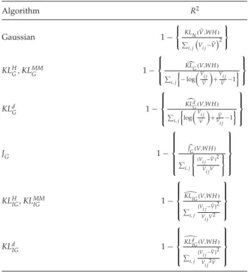
Table 2: Algorithm-Specific Proportion of Explained VariationR2_. Algorithm R2 Gaussian 1− KL_N(Vˆ,WH) i,j V_{i j}− ¯V2 KLH G,KLMMG 1− ⎧ ⎨ ⎩ KL_G(V,WH) i,j −log _V i j ¯ V +Vi j ¯ V −1 ⎫ ⎬ ⎭ KLd G 1− ⎧ ⎪ ⎨ ⎪ ⎩ KLd G(V,WH) i,j log _V i j V +V¯ V_{i j}−1 ⎫ ⎪ ⎬ ⎪ ⎭ J_G 1− ⎧ ⎪ ⎪ ⎪ ⎨ ⎪ ⎪ ⎪ ⎩ $ J G(V,WH) i,j ⎧ ⎨ ⎩ (V_{i j}− ¯V)2 V_{i j}V ⎫ ⎬ ⎭ ⎫ ⎪ ⎪ ⎪ ⎬ ⎪ ⎪ ⎪ ⎭ KLH_IG,KLMM_IG 1− ⎧ ⎪ ⎪ ⎨ ⎪ ⎪ ⎩ KL_IG(V,WH) i,j {V_{i j}− ¯V}2 V_{i j}V2 ⎫ ⎪ ⎪ ⎬ ⎪ ⎪ ⎭ KLd IG 1− ⎧ ⎪ ⎪ ⎨ ⎪ ⎪ ⎩ KLd IG(V,WH) i,j {V_{i j}− ¯V}2 V_{i j}2V¯ ⎫ ⎪ ⎪ ⎬ ⎪ ⎪ ⎭

likelihood for NMF is obtained using equation 2.9 and was first proposed by Lee and Seung (2001).

For each algorithm,R2_{is computed based on the corresponding}

min-imum reconstruction error (E), as listed in Table 2. In the R2 _{column of}

this table, the numerator of each quantity within parentheses (other than

the gaussian) is the minimum reconstruction error (E) calculated using

equations 3.2, 3.7, 3.12, 3.15 and 3.18, as appropriate. The quantity(WH)_{i j}in

each numerator is the (i,j)th entry of the reconstructed matrixWH(also

ob-tained asr_a=1W_iaH_{a j}for a given rankr). In the corresponding denominator

of each quantity, each entry of the reconstructed matrixWHis replaced by

the grand mean of all entries of the input matrixV,V¯ = _np1{p_i=1n_j=1V_{i j}}.

The underlying principle in the calculation ofR2 _{is that the}

algorithm-specific reconstruction error E quantifies the performance of the model

as determined by the entries (WH)_{i j}, while in the absence of the model

V∼WH, the best approximation of(WH)_{i j}is provided simply by the grand

mean of all observations in the data. This is a direct extension of the

as the gamma and inverse gaussian. The algorithm-specificR2 _measures

the proportionate reduction in uncertainty due to the inclusion ofWand

Hand, therefore, can be interpreted in terms of information content of the

data (see Cameron & Windmeijer, 1996, 1997, for more details).

4.2 Akaike Information Criterion (AIC). For a particular algorithm

and a prespecified rankr,AICis given by

AIC=2(τE+ψ ), (4.2)

whereEis the corresponding minimum reconstruction error,ψ=(p+n)r

is the total number of parameters estimated in the model for a p×n

in-put matrixV, andτ =_2σ12, αand λ₂ for the gaussian, gamma, and inverse

gaussian models, respectively. The model (rankrfactorization) that results

in the smallest AIC is chosen as the optimal model. The calculation of

algorithm-specificEis detailed in section 4.1, and the determination ofτis

outlined in section 5.

5 Implementation of Algorithms on EMG Data

In this section, we present a detailed application of NMF algorithms based on signal-dependent noise in the analysis of the EMG data described in section 2. Time-invariant muscle synergies were extracted from each of the intact and deafferented EMG data sets of each frog using each of the eight NMF algorithms described earlier, including one based on normally

distributed noise (gaussian), four based on gamma noise (includingKLH

G,

KLMM

G ,KLdG, andJG), and three based on inverse gaussian (IG) noise

(includ-ingKLH

IG,KLMMIG , andKLdIG). The NMF update rules were implemented using

Matlab. It should be noted that none of the preprocessed data sets contained

zero entries. For every extraction, the muscle synergies (W) and their

asso-ciated time-varying activation coefficients (H) were initialized with random

matrices whose components were uniformly distributed between 0 and 1. Convergence was defined as having 20 consecutive iterations with a change

ofR2_{smaller than 10}−8_(withR2_{for each algorithm defined in Table 2), but}

if convergence was not reached within 500 iterations, the extraction was

terminated. The number of muscle synergiesrextracted from each data set

was successively increased from 1 to 13; at each number, extraction was repeated 20 times, each time with different random initial matrices.

AIC was calculated as follows. Let c denote the parameter 2σ2_{, α, or}

λ/2 depending on the model. In the specification of the divergence for

each algorithm (see section 2.2.2, equations 2.9 to 2.14), we assumed that

c=1 without loss of generality. In order to ensure that the EMG data

fit this assumption, a global test of the null hypothesisH₀:c=1 against

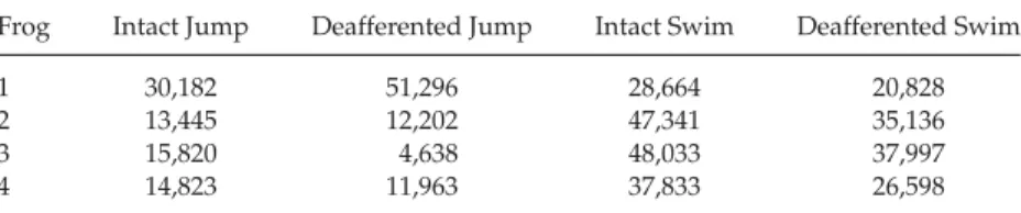
Table 3: Dimensionality of the Data Set for Each Frog and Behavior: Number of Columnsninψ=(p+n)rfor CalculatingAICin Equation 4.2.

Frog Intact Jump Deafferented Jump Intact Swim Deafferented Swim

1 30,182 51,296 28,664 20,828

2 13,445 12,202 47,341 35,136

3 15,820 4,638 48,033 37,997

4 14,823 11,963 37,833 26,598

mean-variance relationship for the gamma and inverse gaussian models can be written using equations 2.6 and 2.8, respectively, and is described in detail in section 2.2.3. This relationship was used to obtain an estimate

ofαorλin these models. For the gaussian model,σ2_{was estimated using}

the approach described in Morup and Hansen (2009). In addition, these parameters were estimated using standard maximum likelihood methods.

In each case, the estimate ofcwas approximately 1, and the 95% confidence

interval for this estimate included 1, (p-values for these tests ranged from

0.15 to 0.77) thereby providing strong evidence in favor of the null

hypoth-esisc=1. Based on this empirical evidence, cwas taken to be 1 and the

appropriate value ofτ was used in equation 4.2 for each model. The best

model order was selected by identifying the rankrgiving the minimum

AICfor each data set and algorithm. Table 3 lists the dimensionality of the

data set, that is, number of columnsninψ in equation 4.2, for each frog

and behavior.

Since for this application we are primarily interested in the ability of each algorithm to identify features shared between the intact and deaf-ferented EMG data sets (or features interpretable as units of CPGs), the performance of each algorithm was assessed by the similarity between the intact and deafferented muscle synergies, quantified with two measures. The first measure used was the scalar product between best-matching pairs of intact and deafferented synergies, calculated after the synergies were normalized to unit vectors. The second measure used was the cosine of the principal angles between the subspaces spanned by the intact and deaffer-ented synergy sets (Golub & Van Loan, 1983). Both measures were used in Cheung et al. (2005).

5.1 NMF Algorithms Based on Signal-Dependent Noise Outperfor-med Gaussian NMF. In analysis of motor patterns from natural behaviors, it has remained difficult to determine, a priori, the number of muscle syn-ergies composing the data set. Most previous studies on muscle synsyn-ergies have relied on ad hoc measures to determine this number either by locating

the cusp of theR2_{curve plotted against the rankr(d’Avella, Saltiel, & Bizzi,}

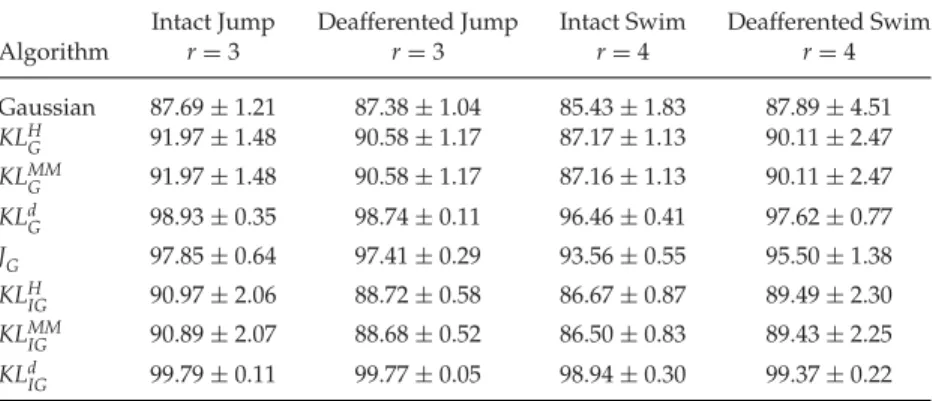
Table 4: The Proportion of Explained Variation (R2_{) Achieved by the NMF} Algorithms in Four Frog Behaviors at the Rank Determined by theJGAlgorithm.

Intact Jump Deafferented Jump Intact Swim Deafferented Swim

Algorithm r=3 r=3 r=4 r=4 Gaussian 87.69±1.21 87.38±1.04 85.43±1.83 87.89±4.51 KLH G 91.97±1.48 90.58±1.17 87.17±1.13 90.11±2.47 KLMM G 91.97±1.48 90.58±1.17 87.16±1.13 90.11±2.47 KLd G 98.93±0.35 98.74±0.11 96.46±0.41 97.62±0.77 J_G 97.85±0.64 97.41±0.29 93.56±0.55 95.50±1.38 KLH IG 90.97±2.06 88.72±0.58 86.67±0.87 89.49±2.30 KLMM IG 90.89±2.07 88.68±0.52 86.50±0.83 89.43±2.25 KLd IG 99.79±0.11 99.77±0.05 98.94±0.30 99.37±0.22

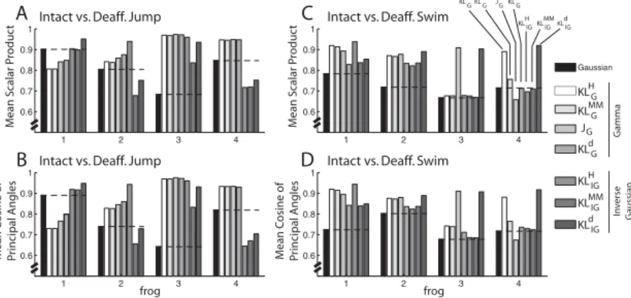
theJ_G algorithm exceeded that of the gaussian algorithm in three of four

frogs in the jump data sets (frogs 2, 3, 4; see Figures 4A and 4B) and also in three of four frogs in the swim data sets (frogs 1, 2, 3; see Figures 4C and 4D). Overall, the three best-performing algorithms in terms of these measures

wereJ_G(mean scalar product=0.8698;N=4×2=8);KLd

IG(0.8695), and

KLH

G(0.8650). The worst-performing algorithm was gaussian (0.7648).

Table 5 lists the proportion of explained variance (R2_{) achieved by the}

NMF algorithms at the ranks with minimumAIC. For every algorithm, the

number of muscle synergies underlying each behavior of each frog was

determined by selecting the rank that resulted in the smallestAICvalues.

AllR2_{values shown are averages across frogs (N=4; mean±SD).}

It is clear from the results shown in Tables 4 and 5 that all three pro-posed algorithms outperformed existing algorithms in terms of fraction of

explained variation (R2_{), both at the ranks with minimumAICand at the}

ranks determined by theJ_Galgorithm. A closer look also revealed that the

variability of this fraction (estimated by the standard deviation) was sig-nificantly lower for the proposed algorithms relative to existing methods, indicating a higher overall confidence level in the variation explained by

these methods. TheJ_Galgorithm provided a much better balance between

R2_{and choice of rank based on minimumAICcompared to any other}

al-gorithm. The ranks chosen by theKLd

Galgorithm based on minimumAIC

were similar to those of existing gamma-based algorithms; however, this al-gorithm was able to explain a much higher fraction of variation in the data.

TheKLd

IGalgorithm explained the maximum variation (highest overallR2)

among all algorithms, while the gaussian algorithm provided the smallest

R2 _{and rank. Furthermore, the variability ofR}2 _{was also the highest for}

the gaussian algorithm, suggesting an overall lower confidence level in the variation explained by this algorithm.

M

ean C

osine of

P

rincipal Angles _Mean C

osine of P rincipal Angles M ean Scalar P roduc t M ean Scalar P roduc t A B C D Intact vs. Deaff. Jump

Intact vs. Deaff. Jump

Intact vs. Deaff. Swim

Intact vs. Deaff. Swim

Figure 4: Signal-dependent noise NMFs outperformed the gaussian NMF. In this application, we are primarily interested in each algorithm’s ability to iden-tify structures shared between the intact and deafferented data sets; thus, our measures of algorithm performance are based on quantifying the similarity be-tween the intact and deafferented muscle synergies. For both the scalar-product (A and C) and principal angle (B and D) measures, overall the seven NMFs based on signal-dependent noise outperformed the gaussian NMF in their abil-ity to extract features shared between data sets. In each graph, the level of similarity achieved by the gaussian algorithm (black) is marked by a horizontal black dotted line for ease of visual inspection.

5.2 Muscle Synergies Extracted by theJ_GAlgorithm Were Physiologi-cally Interpretable. In this section, we compare swim muscle synergies ex-tracted using the standard gaussian algorithm with those identified by the

J_Galgorithm in one specific individual (frog 2) and illustrate how the latter

set could be more physiologically interpretable. In the extraction results returned by the gaussian formulation, a very high similarity between the pre- and postdeafferentation synergies was observed in two of the synergy

pairs (scalar product >0.90; see Figure 5A, synergies 1 to 2), a

moder-ate similarity in one synergy pair (scalar product=0.90; see Figure 5A,

synergy 3), and total dissimilarity in the last pair (scalar product=0.06; see

Figure 5A, synergy 4). By contrast, theJ_Galgorithm found three synergy

pairs with high similarity (scalar product>0.90; see Figure 5B, synergies

1 to 3); in the last pair, the similarity was modest (scalar product=0.62;

see Figure 5B, synergy 4), but the muscles active in both the intact and deafferented synergy vectors were the same (RI, AD, SM, and ST). Overall,

the synergy extraction results from this frog demonstrate that theJ_G

algo-rithm, derived from a signal-dependent noise assumption, is better able to discover structures preserved after deafferentation than the traditional gaussian algorithm.

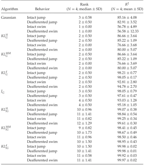
Table 5: The Proportion of Explained Variation (R2_{) Achieved by the NMF} Algorithms at the Ranks with MinimumAIC.

Rank R2

Algorithm Behavior (N=4; median±SD) (N=4; mean±SD)

Gaussian Intact jump 3±0.58 85.16±4.08

Deafferented jump 2±0.50 82.91±3.52 Intact swim 1±0.00 56.78±4.89 Deafferented swim 1±0.00 56.58±12.33 KLH_G Intact jump 2±0.50 86.66±3.64 Deafferented jump 2±0.50 85.22±1.09 Intact swim 2±0.00 76.66±3.68 Deafferented swim 2±0.00 80.00±5.07 KLMM G Intact jump 2±0.50 86.66±3.64 Deafferented jump 2±0.50 85.22±1.09 Intact swim 2±0.00 76.66±3.69 Deafferented swim 2±0.00 80.00±5.07 KLd G Intact jump 2±0.50 98.21±0.77 Deafferented jump 2±0.50 98.05±0.17 Intact swim 2±0.50 92.81±2.80 Deafferented swim 2±0.50 94.78±2.70 J_G Intact jump 3±0.50 98.05±0.79 Deafferented jump 3±0.50 97.61±0.47 Intact swim 4±0.50 93.03±1.28 Deafferented swim 4±0.50 95.18±1.05 KLH_IG Intact jump 10±0.96 99.07±0.38 Deafferented jump 11±1.41 98.84±0.54 Intact swim 11±0.82 99.25±0.34 Deafferented swim 12±1.29 99.61±0.30 KLMM IG Intact jump 9±0.82 98.41±0.45 Deafferented jump 10±1.73 98.67±0.49 Intact swim 11±0.96 98.50±0.46 Deafferented swim 10±1.50 98.95±0.43 KLd IG Intact jump 10±1.50 99.98±0.02 Deafferented jump 10±1.41 99.98±0.01 Intact swim 11±0.58 99.92±0.03 Deafferented swim 11±1.41 99.97±0.02

The muscular compositions of the synergies returned by theJ_Galgorithm

could also be biomechanically interpreted, Synergy 3 (see Figure 5B), for instance, was composed of the hip extensor SM; knee extensors VI, RA, and VE; and the ankle extensor GA. Examination of the time-varying coefficients associated with this synergy revealed that it was active only during the extension phase of every swim cycle; thus, it is likely that muscle synergy 3 functions to propel the animal forward through extension of the hip, knee, and ankle joints. Synergy 1 (see Figures 5A and 5B), discovered by both the

(see Figures 5A and 5B), on the other hand, consisted primarily of the ankle flexors TA and PE, and the hip/knee flexor SA. It is no surprise that both of these synergies were active during the flexion phase of every swim cycle.

The activation pattern of synergy 4 identified byJ_G(see Figure 5B) was

more complex. During the intact state, it was primarily active during limb flexion; after deafferentation it was activated only during limb extension. Consistent with this switch of activation phase for this synergy after the loss of sensory feedback, the correlation coefficient between the activation coefficients of synergy 4 and those of the extension synergy 3 increased five-fold after deafferentation (see Figure 5C). Since three muscles in this synergy—RI, SM, and ST—have both hip extension and knee flexion ac-tions, it is possible that before deafferentation, this synergy executes knee flexion, while after deafferentation, it aids limb extension. It thus appears that sensory feedback functions both to inhibit its activation during exten-sion and facilitates or triggers its activation during flexion. Such an inference about the contribution of afferents to the inhibition and activation of this muscle synergy would be difficult with the synergy sets obtained by the gaussian NMF (see Figure 5A) given that the gaussian algorithm failed to discover this synergy from the deafferented data set.

5.3 Comparison of Results Using Algorithms Derived from the Same Noise Distribution. In the preceding sections, we compared the

perfor-mance of various algorithms in extracting muscle synergies based onAIC,

the fraction of explained variation (R2_{), their ability to identify features}

shared between the deafferented and intact EMG data (measured by the scalar dot product and cosine of the principal angle), and their physiolog-ical interpretability. In this section, we perform a comparison of muscle synergies extracted by different NMF algorithms from the same EMG data set in order to understand how the underlying noise assumption and cost function used in the NMF algorithm may affect the muscular compositions of the extracted synergies. Algorithms based on the same noise distribution but different cost functions tended to return similar muscle synergies. For

instance, when we use KLH

G andKLHIG as reference algorithms, the scalar

product values (mean ± SD; over four frogs) between the synergies

re-turned by gamma-based NMF algorithms and KLH

G were (1) higher than

those between the synergies returned by the gaussian NMF algorithm and KLH

G and (2) higher than those between inverse gaussian-based NMF

al-gorithms and KLH

G (see Figure 6A). Similarly, the scalar product values

(mean ±SD; over four frogs) between the synergies returned by inverse

gaussian-based NMF algorithms andKLH

IGwere (1) higher than those

be-tween the synergies returned by the gaussian NMF algorithm andKLH

IGand

(2) higher than those between gamma-based NMF algorithms andKLH

IG(see

Figure 6B).

Our analysis shows that in our frog EMGs, algorithms derived from the same noise distributions tended to return similar muscle synergies. The

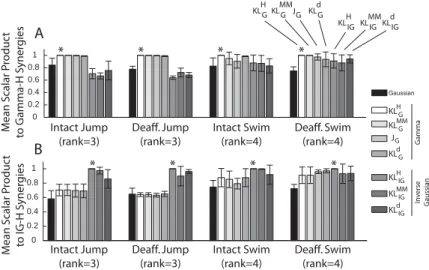
0 0.2 0.4 0.6 0.8 1 0 0.2 0.4 0.6 0.8 1 Intact Jump (rank=3) Deaff. Jump (rank=3) Intact Swim (rank=4) Deaff. Swim (rank=4) M ean Scalar P roduc t to IG-H S yner gies M ean Scalar P roduc t to G amma-H S yner gies Intact Jump (rank=3) Deaff. Jump (rank=3) Intact Swim (rank=4) Deaff. Swim (rank=4) A B

Figure 6: Comparison of results using NMF algorithms derived from the same noise distribution. We performed a comparison of the muscle synergies ex-tracted by different NMF algorithms from the same EMG data set in order to understand the effects of the NMF-noise distribution and the cost function em-ployed on the muscular compositions of the extracted muscle synergies. (A) In each frog, the set of muscle synergies extracted by each algorithm was matched to the set returned by the gamma-basedKLH

G algorithm (*), and their similarity was quantified by the scalar product values averaged across the synergy set. Shown in the plot are values averaged across frogs (N=4; mean±SD). Values for theKLH

G were 1.0 by definition. In this comparison, scalar product values from the gamma algorithms tended to be higher than those from the gaussian or IG-based algorithms. This difference is especially obvious for the intact jump and deafferented jump data sets. (B) Same as panel A, except that the com-parison was performed by matching synergies of each algorithm to synergies returned by the IG-basedKLH

IGalgorithm (*). In this comparison, scalar product values from IG-based algorithms tended to be higher than those from the gaus-sian or gammabased algorithms. Again, this difference is especially obvious for the intact jump and deafferented jump data sets.

noise distribution appears to play a critical role in determining the muscular compositions of the synergies extracted from the data. Similarly, the cost function (divergence measure) employed for formulating the update rules exerts its own influence on the extraction results. Indeed, the best rank

(rank with minimalAIC) andR2_{values from algorithms assuming the same}

noise distribution but employing different cost functions were still different (see Table 5). This is because these algorithms derived from different cost

functions returned different activation coefficients (H). As an illustrative

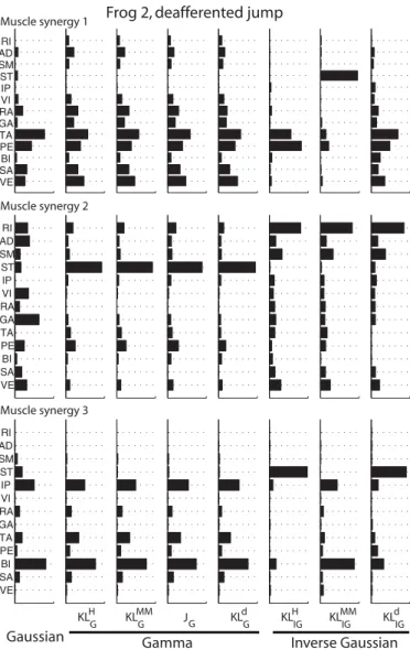
Figure 7: Both the noise distribution and the cost function employed for formu-lating the NMF update rules could influence the muscular compositions of the extracted muscle synergies. Here we show the muscle synergies extracted from one particular data set (frog 2, deafferented jump) by different NMF algorithms. The results returned by the four gamma-based algorithms were almost iden-tical (as suggested by Figure 6). However, the gamma synergies were clearly different from the gaussian and IG-based synergies. Also, the muscle synergies returned by the three IG-based synergies were also somewhat different from each other. Thus, both the noise distribution and the cost function used for de-riving the NMF update rules could influence the structures of the basis vectors extracted.

algorithms from the deafferented jump EMGs of frog 2. In this case, the results produced by the four gamma-based NMF algorithms are nearly identical. However, it is important to note that the synergies extracted by the three IG-based NMF algorithms are quite different, exposing the activation of different muscles as determined by the choice of cost function.

6 Evaluating NMF Algorithms on Simulated Data Sets

In this section, we present a detailed application of the proposed NMF al-gorithms to the analysis of simulated data. We implemented the alal-gorithms

on simulated data sets generated by known muscle synergies (W) and

time-varying activation coefficients (H), so that the performance of each NMF

algorithm can be evaluated by comparing the extracted results with the

originalWandH.

In our simulations, we are interested in how well each algorithm per-forms as a function of noise distribution and noise level in the data. For every distribution and noise amplitude tested, 10 simulated data sets were generated. Each data set, consisting of 15 muscles and 5000 time points, was produced by linearly combining five muscle synergies. The

compo-nents of bothW andHwere drawn from a uniform distribution defined

over (0,1). The simulated data were then corrupted by one of the three

noise types—gaussian, gamma, and inverse gaussian—at different noise

magnitudes quantified by the signal-to-noise ratio (SNR), defined as

SNR= i,jVi j2 i,j(Vi j− ˜Vi j) 2,

where V_ij is the original, uncorrupted data point and V˜_{i j} is the

noise-corrupted data point. For gaussian noise with mean μand varianceσ2_,

noise for each data point was generated by the Matlab function,normrnd,

withμ=V_{i j} andσ set to 0.04, 0.05, 0.07, 0.1, 0.2, 0.3, 0.5, 1.0, 1.5, and 2.0,

respectively. These choices ofσproduced data with anSNRranging from

0.17 to 225. For gamma noise with mean α_β (see equation 2.5), the Matlab

functiongamrndwas used, withβ=_Vα

i j andαset to 0.1, 0.5, 0.25, 1.0, 2.5,

5.0, 10, 50, 100, 250, and 500, respectively (SNRof 0.1 to 500). For inverse

gaussian noise with meanμ(see equation 2.7), noise for each data point

was generated by combining the Matlab functionsmakedist andrandom,

withμ=V_{i j}andλset to 0.1, 0.2, 0.5, 0.75, 1, 2, 5, 7, 10, 12, 14, 16, 18, 20, 30,

40, and 100, respectively (SNRof 0.14 to 139).

The eight NMF algorithms described in this letter (gaussian,KLH

G,KLMMG ,

KLd

G,JG,KLHIG, KLMMIG , and KLdIG) were then applied to each of the

simu-lated data sets for extracting five muscle synergies. In every extraction, the

matrices were initialized with random components drawn from a uniform

distribution over(0,1). Convergence was defined as having 20

consecu-tive iterations with a change of algorithm-specificR2_{(see Table 2) smaller}

than 10−8, but if convergence was not achieved within 500 iterations, the

extraction was terminated. Extraction was repeated 20 times for each data set, each time with different initial random matrices. The extraction repe-tition with the smallest reconstruction error among the 20 reperepe-titions was then selected for performance evaluation. The ability of each algorithm in identifying the muscle synergies was quantified by the scalar product be-tween the original and extracted synergy vectors (after the synergies were normalized to unit vectors), averaged over the five synergies. For the acti-vation coefficients, performance was assessed by the Pearson’s correlation

coefficient (ρ) between the components in the originalHand those in the

extractedH, again averaged over the five synergies.

For gaussian-noise data sets, the gaussian algorithm outperformed KLd

G,JG, and all IG-based algorithms in the identification of both Wand

H (see Figure 8; *, p<0.05; Student’s t-test). The superiority in

perfor-mance of the gaussian NMF over all other algorithms was especially

ob-vious for the extraction of H (see Figure 8B). For the extraction of W,

however, the performances of gaussian,KLH

G, and KLMMG were

compara-ble (see Figure 8A).

In data sets with simulated gamma noise, the gamma- and IG-based algorithms performed equally well, and better than gaussian, in the

identi-fication ofHover all tested noise magnitudes (see Figure 9B). ForW

identi-fication, the gamma- and IG-based algorithms were similar in performance

when theSNRwas above≈3 (see Figure 9A). The gamma algorithms

out-performed all other algorithms when noise magnitude was very high (see

Figure 9A; +,p<0.05).

In data sets corrupted by inverse gaussian noise, forWidentification,

not surprisingly the IG-based algorithms outperformed the gamma-based algorithms (see Figure 10A; *), which in turn outperformed the gaussian

(see Figure 10A; +, *). ForHidentification, while the performances of all

signal-dependent noise NMFs were almost indistinguishable, they clearly did much better than the gaussian (see Figure 10B, *).

Overall, the simulation results highlight the need for using the NMF al-gorithm derived from a noise distribution that matches the noise type of the

data for the most accurate identification of bothWandH. However, under

certain conditions, even when the noise assumed by the NMF algorithm and the data noise type do not completely agree, the extracted results may still contain substantial information about the underlying data structure. We have seen, for instance, that in data with gamma noise, IG-based NMF algorithms could identify muscle synergies as well as gamma-based NMF

algorithms could. It should be noted that even when the identified Wis

reasonably close to the original generating bases, theHidentified by the