Design and Stability Analysis of Multi-Objective Ensemble Classifiers

Correspondence to: [email protected] Recommended for acceptance by Angel Sappa http://dx.doi.org/10.5565/rev/elcvia.929

ELCVIA ISSN: 1577-5097

Published by Computer Vision Center / Universitat Autonoma de Barcelona, Barcelona, Spain

Design and Stability Analysis of Multi-Objective Ensemble

Classifiers

Zeinab Khatoun Pourtaheri

*

Seyed-Hamid Zahiri

*

and Seyed Mohammad Razavi

* * Department of Electrical and Computer Engineering,University of Birjand, Birjand, Iran

[email protected], [email protected], [email protected] Received 21st May 2016; accepted 30th Dec 2016

Abstract

In this paper a novel multi-objective optimization technique based on Inclined Planes Optimization algorithm (called MOIPO), is used to design an ensemble classifier. Diversity, ensemble size, and error rate are three objectives which are considered along designing the proposed ensemble classifier.

The performance of designed ensemble classifier is tested on different kinds of benchmarks with nonlinear, overlapping class boundaries, and different feature space dimensions. Extensive experimental and comparative results on these data sets provided to show the performance of the proposed method, are better than ensemble designed by Multi-Objective Particle Swarm Optimization (MOPSO) algorithm.

Another important aspect of this article is stability analysis of designed ensemble classifier. In fact, for the first time, the stability of a heuristic ensemble classifier is analyzed by using statistical method. For this aim, three regression models are investigated by applying F-test to find better model in each case. Due to the results of stability analysis, quadratic model is the best model for two datasets as representative of simple data and overlapped data.

Key Words: Ensemble Classifier, Heuristic Algorithms, Multi-Objective Inclined Planes Optimization Methods, Regression Models, Stability Analysis.

1

Introduction

Ensemble method is one of the main developments in machine learning in the past years. An ensemble classifier contains a group of individually trained classifiers whose predictions are combined when classifying new samples [1]. In other words, an ensemble classifier combines a finite number of classifiers of the same type or different, trained concurrently for a joint classification problem. The ensemble efficiently amends the performance of the classifier compared to a single classifier [2].

On the first step of designing an ensemble classifier, several base classifiers, which are usually traditional and known classifiers in pattern recognition, are used. At this point, the designer should employ a collection of complementary base classifiers which can cover the weakness of each other by making independent and supplementary decisions. Thus, as regards to the diversity among base classifiers is an important factor for

achievement of ensemble classifier systems, and considering that the classifiers are built in a learning process and on the other hand, in order to have diverse base classifiers, it's necessary to make the learning process of base classifiers different; this task can be attained in various methods. Finally, the outcome of this step is a pool of base classifiers.

There are two main techniques when dealing with ensemble classifiers: fusion and selection. In the first, it's expected that each classifier has independent error. Of course, it's difficult to inflict independence among the components of ensemble because base classifiers are redundant [3]. Since they obtain the answer to an equivalent problem, there is no assurance that a specific ensemble combination method attains independent error [4]. By contrast, the aim of classifier selection is to find the most efficient subset of classifiers instead of combining all existing classifiers and this method is applied in this paper.

In designing an ensemble classifier, there are a variety of significant topics which affect directly on the performance of the designed ensemble classifier. Some of instances in this issue include: number and kind of base classifiers, training technique, method of making final decision and combining decisions, feature selection (possibly feature fusion), even, the ultimate aim of designing an ensemble classifier. These problems make a complex search space with high dimensions so it is often impossible to find the best solution in such space by using trial and error. On the other hand, heuristic algorithms have the capability to search the solution space efficiently and thus, they can find best solutions. So, the use of such algorithms is proposed to design ensemble classifiers.

Heuristic algorithms sometimes receive various solutions in different simulation runs due to the random nature of them. These responses are highly dependent on the structural parameters of employed algorithms. An important issue in the literatures of heuristic algorithms application is stability which means how much the changes of structural parameters influence the output of heuristic methods.

Several researches have addressed the stability analysis of heuristic algorithms; in [5] a stability analysis of the stochastic particle dynamics in particle swarm optimizer is provided. The analysis is made feasible by representing the particle dynamics as a nonlinear feedback controlled system as formulated by Lure. The impacts of tuning parameters on the performance of genetic algorithm have been evaluated in [6] by using regression modeling. An elite reservation technique for the robust GA, which performs random perturbation during optimization processes, has been applied in [7].

Since, there is no study related to stability of multi-objective heuristic ensemble classifiers, in this paper, for the first time, the stability of these systems is investigated by using statistical analysis. In order to accomplish this, in the first step, two multi-objective heuristic algorithms, named Multi-Objective Inclined Planes Optimization (MOIPO) and Multi-Objective Particle Swarm Optimization (MOPSO), are used to design ensemble classifiers. Then, the performance of these ensemble classifiers is studied in terms of three objective functions including ensemble size, error rate and diversity. Finally, stability analysis of the best ensemble classifier is done.

The rest of this paper is organized as follows: Section 2 provides the related works. In section 3, the technique of stability analysis, which is used in this research, is presented. Section 4 reviews the employed multi-objective heuristic algorithms. Section 5 explains how to design multi-objective heuristic ensemble classifiers and implement the stability analysis of the best one. Section 6 discusses the results and finally Section 7 is devoted to conclusions.

2

Related Works

There are several ensemble approaches for combining a set of classifiers. Among them, boosting [8] and bagging [9] are two important methods which have been widely used.

Boosting changes the distribution of weights of each training sample. Initially the weights are uniform for all the training samples [10]. This approach increases weight on the misclassified samples through iterations. The samples that are incorrectly classified by previous classifiers are selected more often than samples that are correctly classified. So Boosting tries to produce new classifiers which are better able to classify samples for which the present ensemble’s performance is poor. Boosting combines predictions of ensemble of classifiers with weighted majority voting by giving more weights on more accurate predictions [11].

In Bagging procedure, the training subsets are randomly selected (with replacement) from the original training set. Similar base classifiers are trained on the subsets. Base classifiers are then combined by using majority vote of their decisions. The final decision of the ensemble classifier is the class chosen by most base classifiers. There are a number of variants of bagging including random forests [12]. A random forest can be created from individual decision trees, whose certain training parameters vary randomly. Such parameters can be bootstrapped replicas of the training data, as in bagging, but they can also be different feature subsets as in random subspace methods [13].

Several studies have addressed these types of ensemble classifiers; in [14] an in-depth analysis of a random forests model is offered. This paper shows that the procedure is consistent and adapts to sparsity, in the sense that its rate of convergence depends only on the number of strong features and not on how many noise variables are present. Skurichina and Duin in [15] indicate that bagging, boosting and the random subspace method can be beneficial in linear discriminant analysis. Simulation results show that the performance of the combining methods is strongly affected by the small sample size properties of the base classifier: boosting is useful for large training sample sizes, while bagging and the random subspace method are useful for critical training sample sizes. In [16] a way to manage the learning complexity and improve the classification performance of AdaBoost.MH is provided and called RFBoost. The weak learning in RFBoost is based on filtering a small fixed number of ranked features in each boosting round rather than using all features, as AdaBoost.MH does. A novel approach for bankruptcy prediction that applies Extreme Gradient Boosting for learning an ensemble of decision trees is proposed in [17]. The connection between the random forests and the kernel methods is provided in [18]. It shows that by slightly modifying their definition, random forests can be rewritten as kernel methods (called KeRF for kernel based on random forests) which are more interpretable and easier to analyze. A novel approach for improving Random Forest in hyper spectral image classification is proposed in [19]. The proposed approach combines the ensemble of features and the semi-supervised feature extraction technique.

Besides the mentioned methods, there is a great trend to heuristic approaches; three meta-heuristic approaches for the optimization of stacking configuration are studied in [20] in which, accuracy is used to compare the results. In [21] first, an optimized static ensemble selection approach is proposed on the basis of NSGA-II multi-objective genetic algorithm by simultaneous optimization of error and diversity objectives. In the second phase, the dynamic ensemble selection-performance is improved by utilizing the first proposed method. A multi-level approach using genetic algorithms is proposed in [22] to build the ensemble of least squares support vector machines. To analyze the performance of the proposed method, they prepared two new versions of the fitness function; the first version uses only the bad diversity calculation while the second consists of the quadratic error norm of the ensemble plus the value of bad diversity.

Heuristic methods have random parameters and their response can be influenced by these structural parameters. Despite the high tendency in designing heuristic ensemble classifiers, there has been no research related to the stability analysis of these systems. So in this paper, for the first time, the stability of these systems is investigated by using statistical analysis which is described in detail in the next section.

3

Statistical Analysis of Stability

Response surface methodology (RSM) is a set of mathematical and statistical methods beneficial for developing, improving, and optimizing processes [23]. The most extensive applications of RSM are in the cases where multiple input variables potentially impress some performance measures or quality characteristics of the process which is called the response. The input variables are sometimes named independent variables and they are subject to the control of the scientist or engineer, at least for the goals of a test or an experiment.

In general, assume that the scientist or engineer (the experimenter) is concerned with a process involving a response y that pertains to the controllable input variables ξ1, ξ2, …, ξk. The relationship is shown in the

following:       f( ₁, ₂,..., _k) y (1)

Where the form of the true response function f is unknown and probably very complex, and is a term that indicates other sources of variability not considered in f. is treated as a statistical error, often assuming to have a normal distribution with mean zero and variance σ2. So the response function is:



( , ,..., )



( ) ( , ,..., )

)

(y E f _{1 2 k} E f _{1 2 k}

E           (2)

In much RSM works, it is appropriate to transform the controllable input variables to coded variables x1,

x2, …, xk, which are usually described to be dimensionless with mean zero and the same standard deviation.

In terms of the coded variables, the true response function (2) is now specified as:

) ,..., , (x₁ x₂ x_k f   (3)

The form of the true response function f must be approximated because it is unknown. In fact, prospering use of RSM is critically dependent upon the experimenter’s ability to develop a proper approximation for f.

It's worth noting that there is a close relationship between RSM and linear regression analysis. For example, consider the following model:

           x x _kx_k y _{0 1 1 2 2} ... (4)

The β’s are a collection of unknown parameters. To assess the values of these parameters, one must gather data on the system under study. Regression analysis is a branch of statistical model building that utilizes these data to estimate the β’s. In general, polynomial models are linear functions of the unknown β’s, so the technique is mentioned as linear regression analysis [24]. In the following subsections linear regression models and F-test for significance of regression are described in details.

3.1 Linear Regression Models

One can fit a response surface for predicting y at various combinations of the design factors. In general, linear regression methods are used to fit these models to the experimental data [25].

For example, a first-order response surface model, which is a multiple linear regression model with two independent variables, is shown in the following:

        _{0 1}x_{1 2}x₂ y (5)

It is very important that one learns to interpret the coefficient estimates both correctly and completely. Sometimes, β1 and β2 are called partial regression coefficients, because β1 measures the expected change in y

per unit change in x1 when x2 is maintained constant, and β2 measures the expected change in y per unit

change in x2 when x1 is maintained constant. The intercept i.e. β0

is the estimate of the mean outcome

when x equals zero [26].

Models which are more complicated in appearance than equation (5) may often be analyzed by multiple linear regression techniques so far. As an example, considering adding an interaction term to the first-order model in two variables:

          _{0 1}x_{1 2}x_{2 12}x₁x₂ y (6)

Let x3=x1x2 and β3= β12, then the equation (6) can be written as a standard multiple linear regression model

with three variables:

          _{0 1}x_{1 2}x_{2 3}x₃ y (7)

In general, any regression model which is linear in the β-values is a linear regression model, irrespective of the shape of the response surface that it produces [25].

The technique of least squares is usually used to assess the regression coefficients in a multiple linear regression model. It says that one should choose as the best-fit line, that line which minimizes the sum of the

squared residuals, where the residuals are the vertical distances from individual points to the best-fit regression line [26].

3.2 F-Test for Significance of Regression

Certain tests of hypotheses about the model parameters are beneficial in measuring the utility of the model in multiple linear regression problems.

The test for significance of regression is a test to specify, if there is a linear relationship, between the response variable y and a subset of the variables x1, x2, …, xk. The appropriate hypotheses are:

j one least at for : H ... : H j k 0 0 1 2 1 0          (8)

Rejection of H0 in equation (8) pointed that at least one of the variables x1, x2, …, xk contributes significantly

to the model [24].

One could use the P-value approach to hypothesis testing and hence, reject H0 if the P-value for the

statistic F0 is less than α which is level of significance. In other words, the p-value is the smallest level of

significance that would lead to rejection of H0 with the given data. This test method is called an analysis of

variance (ANOVA) [27].

The coefficient of multiple determination R2 _{is a measure of the amount of reduction in the variability of y}

achieved by using the variables x1, x2, …, xk in the model. From inspection of the analysis of the variance, it's

obvious that R2 _{varies between 0 and 1. However, a large value of R}2 _{does not necessarily connote that the}

regression model is a good one. Adding a variable to the model will always enhance R2_{, regardless of}

whether the extra variable is statistically important or not.

Because R2 always increases by adding terms to the model, some regression model builders prefer to apply an adjusted R2 _{statistic described as:}

) R ( p n n R_adj2 1 1 1 2     (9)

Where n is the number of observations and p is the number of β’s in the model [24].

It's worth mentioning that, the impact of each variable is determined according to the measured β which is related to it.

4

Multi-Objective Heuristic Algorithms

Heuristic approach is a strategy that disregards some of the information to make decisions rapidly with maximum savings in time and with more precision than of complicated technique [28]. This method guarantees greater probability to reach optimal solutions because it uses a population to explore the problem space [29].

Searching operation in multi-objective heuristic algorithms is accomplished in parallel; means a set of agents search the problem space. So, they can find Pareto-optimal solutions with a single simulation run. These algorithms can save time and also flee from local optimum with special schemes and converge to global optimum.

In multi-objective optimization unlike single-objective optimization, a single solution cannot be introduced as the best solution. In such problems, a set of solutions, which complies each objective function with an acceptable level, is defined as optimal solutions [30].

In this paper, two multi-objective optimization algorithms (called MOIPO and MOPSO) are used and they are defined in the following subsections.

IPO algorithm mimics the dynamic motion of spherical objects along frictionless inclined plane. All of these objects have tendency to reach the lowest points. In this algorithm, the agents are some tiny balls which explore the problem space to find optimal solutions. The main idea of IPO is to impute height to each agent, regarding to its objective function. These heights are estimations of the potential energy of each agent that should be transformed to kinetic energy by assigning suitable acceleration. In fact, agents tend to tine their potential energy and to reach the minimum point(s) [31].

Position, height and angles made with other agents, are three characteristics of each ball in the search space. The position of each ball is a possible solution in the problem space and their heights are acquired using a fitness function.

In a system with N balls, the position of the i-th ball is defined by:



x , ,x , ,x



, fori 1,2, ,N

xi  i1 id  in   (10)

Where, d i

x is the position of i-th ball in the d-th dimension in an n dimensional space. At a given time t, angle

between the i-th ball and j-th one in dimension d, i.e. d ij

φ , is calculated using the following equation:

 

_{ }

 

 

_{ }

j i N, , 1,2, j i, and n , 1, d for , t x t x t f t f tan t i φ _d j d i i j 1 d j                          (11)

Where, fi

 

t is the height (value of objective function) for the i-th ball in time t. Because a specific ball tends

to move toward the lowest heights on the inclined plane, only balls with lower heights (fitness) are used in acceleration calculating.

The amplitude and direction of acceleration for the i-th ball at time t and in dimension d, is measured using:

 

t U



f

   

t f t



.sin

 

φ_i

 

t a d_j N 1 j j i d i     (12)

In which, U()is the Unit Step Function:

Finally, the following equation is used to update the position of the balls:





 

 

t .Δt x

 

t .v rand . k Δt . t a . .rand k 1 t x d i d i 2 2 2 d i 1 1 d i     (13)

rand1 and rand2 are two random weights distributed uniformly on the interval [0,1]. vid

 

t is the velocity of i

-th ball in dimension d, at time t. to control the search process of algorithm, two essential parameters named

k1 and k2 are used. These control parameters of IPO are described as functions of time (t) by using:

 

_

_

_

_

1 1

1 1

1 exp t shift scale

c t k     ₍₁₄₎

 

_

_

_

_

2 2 2 2

1 exp t shift scale

c t k     ₍₁₅₎

Where c1, c2, shift1, shift2, scale1 and scale2 are constants determined for each function, experimentally.

 

t v_id is:

 

 

 

Δt t x t x t v d i d best d i   (16)

In the above equation, d best

x is employed in numerator to determine the ball desire to reach the best position in

any iteration.

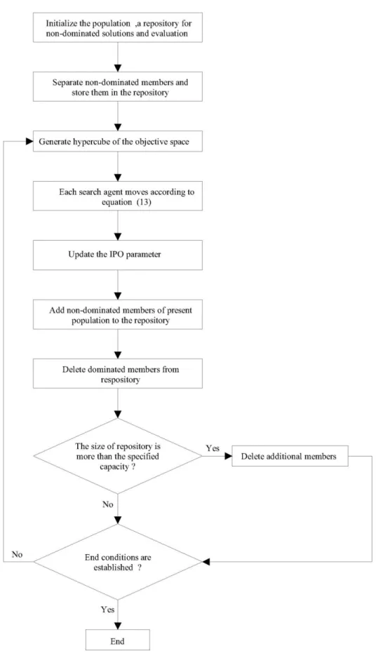
The main structure of the Inclined Planes optimization algorithm should be amended to use it in multi-objective problems [32]. The main steps of multi-multi-objective IPO are shown in the flowchart of Figure 1:

Figure 1: The flowchart of MOIPO algorithm

4.2. Multi-Objective Particle Swarm Optimization (MOPSO) Algorithm

Particle swarm optimization algorithm, which presented by James Kennedy and Russell Eberhurt, is one of the most important intelligent optimization algorithms and stands in the field of swarm intelligence. This algorithm inspires the social behavior of animals like fishes and birds that live in small and large groups [33]. In PSO algorithm, feasible solutions for an optimization problem are considered as birds without volume and quality specifications called particles. These birds fly in an N-dimensional space and change their movement route based on the past experiences of themselves and their neighbors.

The position of the i-th particle in a system contained N particles is demonstrated as:



x ,x , ,x



S

xi  i i  in 

2

1 ₍₁₇₎

In which S is the search space.

The velocity vector and the best remembered individual particle position vector are:



n



i i i i v ,v , ,v v _ 1 2 ₍₁₈₎



n



i i i i p ,p , ,p p _ 1 2 ₍₁₉₎

New particles' positions are acquired by using:

 

 

)) t ( x ) t ( p ( r c )) t ( x ) t ( p ( r c t v t v i g i i i i       2 2 1 1 1  (20) ) t ( v ) t ( x ) t ( x_i 1  _i  _i 1 (21) In above equations: : Inertia weight. g

p : Best remembered swarm position.

1

c : Cognitive parameter.

2

c : Social parameter.

1

r ,r₂ : Random numbers between 0 and 1.

Each particle has a maximum velocity that is specified by user.

Multi-Objective version of PSO can be achieved by applying some changes. In this situation, unlike the single-objective mode, the concept of best particle (best remembered individual particle position) is not fixed but each particle selects randomly a member from the repository as leader per moment. One of the most famous and effective proposal for multi-objective particle swarm optimization algorithm (MOPSO) is introduced in [34]. The steps of MOPSO are similar to MOIPO which was described in the sub-section 4.1. The important differences between MOIPO and MOPSO are the mechanisms of space exploration and employed equations.

5 Design and Stability Analysis of Multi-Objective Heuristic Ensemble

Classifiers

The purpose of this paper is to design multi-objective heuristic ensemble classifiers and also to perform stability analysis which is not addressed in recent researches. So, at first, two multi-objective heuristic ensemble classifiers with three objective functions are designed by exerting MOIPO and MOPSO algorithms then, the victor ensemble classifier is selected for stability analysis. Statistical procedure, which was explained previously in section 3, is used for performing stability analysis. Now, in the following subsections, the way of designing ensemble classifiers and analyzing the stability are explicated.

In the design step, the applied optimization algorithm is looking for the best subset of classifiers, in terms of size, error rate and diversity, among an initial pool of classifier. Thus, ensemble size, error rate and a diversity measure are used as three objective functions to guide the optimization process. It is worth mentioning that in design step, all parameters of the applied algorithms are constant.

Random subspace method is used to create the initial pool of classifiers and k-Nearest Neighbors (kNN) classifiers with k=1 are the base classifiers.

10-fold cross-validation strategy is applied in the experiments; in K-fold cross-validation, K-1folds are used for training and the last fold is used for evaluation. This process is repeated K times, leaving one different fold for evaluation each time.

The specifications of datasets used in the first step, are briefed in Table 1.

Dataset Number of samples Number of features Number of classes Glass Iris Wine Wisconsin 214 150 178 683 9 4 13 9 2 3 3 2 Table 1: Specifications of datasets

In all experiments, population size and number of iterations are considered 20 and 200 respectively. Three important issues should be defined properly when applying heuristic algorithms for optimization: search agents, objective function and combination technique. These issues are explained in the next subsections.

5.1.1 Search Agents Description

Agents' dimensions in both algorithms are twice the size of primary pool of classifiers. Since the primary pool contains 50 classifiers, considered dimensions for search agents will be 100. Dimensions 1 to 50 are coded in binary; ‘1’ means the classifier is selected and ‘0’ means the classifier is not selected. Other dimensions specify coefficients related to each classifier; these coefficients are used in classifier combination process.

5.1.2 Fitness Function Description

Evaluation of each member of the population is done by objective (fitness) function calculation. In this paper, ensemble size, error rate and diversity measure are considered as objective functions to design objective heuristic ensemble classifiers. It's expected these functions will be optimized by using multi-objective heuristic algorithms.

A. Diversity

Diversity among the members of a team of classifiers has been recognized as a key issue in classifier combination. Notwithstanding the popularity of the idiom diversity, there is no single definition and measure of it. Although several measures have been proposed to demonstrate the diversity and are optimized explicitly in different ensemble learning algorithms, none of these measures is proven premier to the others [35].

In this research, the Q statistic is used as a diversity measure and is defined according to [36] in the following.

Let Z={z1,...,zN}be a labeled dataset. The output of a classifier Di can be represented as an N-dimensional

binary vector yi =[y1,i ,... ,yN,i]T, such that yj,i=1 if Di distinguishes correctly zj and 0 otherwise, i =1,...,L.

10 01 00 11 10 01 00 11 N N N N N N N N Q_i,k    (22)

Where Nab _{is the number of elements z}

j of Z for which yj,i=a and yj,k=b (see Table 2).

Dk correct (1) Dk wrong (0)

Di correct (1) N11 N10

Di wrong (0) N01 N00

Table 2: A 2×2 table of the relationship between a pair of classifiers

For an ensemble of L classifiers, the averaged Q statistics over all pairs of classifiers is computed as:





 

     1 1 1 1 2 L i L i k k , i av Q L L Q (23)

It's worth mentioning that the diversity is greater if the Q statistic is lower [37]. B. Ensemble size

Most extant approaches in ensemble learning employ all the trained constitutive classifiers to create ensembles, which are sometimes inessentially large and can propel to extra computational times and costs [10]. One of the objective functions of this paper is ensemble size which is expected to be minimized.

C. Error rate

Classification error rate is used as another fitness function to instruct the optimization process. In fact, recognition rate will be maximized if error rate minimized.

In order to compare the performance of two algorithms in designing ensemble classifiers, three points from Pareto front are selected and compared; these points are an ensemble with minimum size, an ensemble with minimum error rate and an ensemble with maximum diversity.

5.1.3 Combination Technique

When a subset of classifiers is found, a combination technique should be applied. Weighted voting is used in this research as combination rule. The weight of each classifier is characterized by the search agent. If a classifier is selected, its relevant coefficient should be used in combination process.

5.2 Stability Analysis Step

After determining the winner algorithm in the first step, second step i.e. stability analysis starts. To obtain required data for this phase, the algorithm's parameters, which were constant in the previous step, change in the range of 50% and the algorithm is repeated as many as the number of necessary observations.

To perform stability analysis, Iris and Glass datasets are utilized as a representative of simple data and overlapped data respectively.

For stability analysis, six parameters (c1, c2, shift1, shift2, scale1 and scale2) are considered as variables

(coded to x1 to x6, respectively) and three points of Pareto front (ensemble with minimum error rate,

ensemble with minimum size and ensemble with maximum diversity) are chosen for response value (y). Then three regression models are checked by using F-test meanwhile α=0.05. These models are linear, quadratic and cubic which are specified in the following equations respectively:

6 6 1 1 0 x ... x y    (24) 2 6 66 2 1 11 6 6 1 1 0 x ... x x ... x y       (25) 3 6 666 3 1 111 2 6 66 2 1 11 6 6 1 1 0 x ... x x ... x x ... x y          (26)

Next section provides obtained results of two mentioned steps.

6 Experimental Results and Discussion

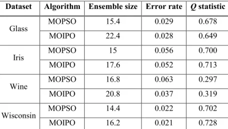
The obtained results of design step are reported in Table 3 to 5. The numerical values of three objective functions in these tables are the average of 5 independent runs. It's worth mentioning that the ensemble in Table 3, Table 4 and Table 5 are an ensemble with minimum size, an ensemble with minimum error rate and an ensemble with maximum diversity respectively.

Dataset Algorithm Ensemble size Error rate Q statistic

Glass MOPSO 7.8 0.033 0.673 MOIPO 7.6 0.043 0.692 Iris MOPSO 12.8 0.057 0.707 MOIPO 5.2 0.063 0.666 Wine MOPSO 11.8 0.076 0.208 MOIPO 7.2 0.057 0.242 Wisconsin MOPSO 11.6 0.023 0.733 MOIPO 7 0.023 0.732

Table 3: Obtained comparative results using MOPSO and MOIPO (Ensemble with minimum size considered as best ensemble)

Due to Table 3, MOIPO performs better than MOPSO for all datasets; the value of ensemble size is smaller when using MOIPO algorithm for designing multi-objective ensemble classifier. In the best case, ensemble size has improvement by 59.38% for Iris by using MOIPO.

Dataset Algorithm Ensemble size Error rate Q statistic

Glass MOPSO 15.4 0.029 0.678 MOIPO 22.4 0.028 0.649 Iris MOPSO 15 0.056 0.700 MOIPO 17.6 0.052 0.713 Wine MOPSO 16.8 0.063 0.297 MOIPO 20.8 0.037 0.319 Wisconsin MOPSO 14.4 0.022 0.702 MOIPO 16.2 0.021 0.728

Table 4: Obtained comparative results using MOPSO and MOIPO (Ensemble with minimum error rate considered as best ensemble)

According to Table 4, for all datasets, MOIPO has outperformed MOPSO in terms of error rate values. For Wine, MOIPO compared with MOPSO leads to 41.27% improvement.

Dataset Algorithm Ensemble size Error rate Q statistic Glass MOPSO 14 0.035 0.590 MOIPO 12.4 0.045 0.530 Iris MOPSO 17.2 0.059 0.673 MOIPO 8.8 0.067 0.589 Wine MOPSO 9.4 0.076 0.376 MOIPO 8.6 0.058 0.173 Wisconsin MOPSO 15.8 0.023 0.665 MOIPO 11.2 0.023 0.629

Table 5: Obtained comparative results using MOPSO and MOIPO (Ensemble with maximum diversity considered as best ensemble)

According to Table 5, the value of Q statistic is better when using MOIPO. Obtained improvement of this measure is up to 53.99%.

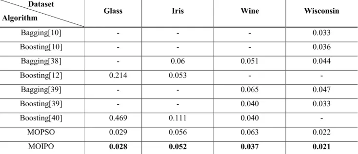
Up to now, experimental results confirm that MOIPO, as a novel multi-objective optimization, has high capability to design multi-objective heuristic ensemble classifier with improved values of considered objective functions. So, this algorithm is selected for next step i.e. stability analysis. In order to provide a comparison between proposed ensemble classifier and existing methods, the obtained error rate in Table 4 is compared with obtained error rate using Bagging and Boosting methods in Table 6.

Dataset

Algorithm Glass Iris Wine Wisconsin

Bagging[10] - - - 0.033 Boosting[10] - - - 0.036 Bagging[38] - 0.06 0.051 0.044 Boosting[12] 0.214 0.053 - - Bagging[39] - - 0.065 0.047 Boosting[39] - - 0.040 0.033 Boosting[40] 0.469 0.111 0.040 - MOPSO 0.029 0.056 0.063 0.022 MOIPO 0.028 0.052 0.037 0.021

Table 6: A comparative analysis of error rate between the proposed ensemble classifier and other methods Table 6 provides a comparative analysis of error rate between the proposed ensemble classifier and existing methods such as Bagging and Boosting. According to this Table, MOIPO outperforms other methods for all datasets.

Another important issue is that there is no explicit measure of diversity involved in the process of Boosting and Bagging but it is assumed that diversity is a key factor for the success of these algorithms [37]; diversity in a bagging-based ensemble classifier was achieved by training the base classifiers using different randomly drawn (with replacement) subsets of data. On the other hand, a boosting-based ensemble classifier was used to create data subsets for base classifier training [41]. However diversity is considered as a measure in the proposed heuristic ensemble classifier and can be optimized during iterations. Also, it’s worth noting that Bagging and Boosting are full ensembles because they use all trained component classifiers but the proposed ensemble uses a subset of the full ensemble.

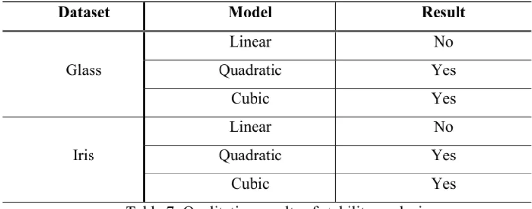
Table 7, summarizes the qualitative results of stability analysis regard to R2_{; means which model is good}

in each case.

Dataset Model Result

Glass Linear No Quadratic Yes Cubic Yes Iris Linear No Quadratic Yes Cubic Yes

Table 7: Qualitative results of stability analysis

As Table 7 shows, quadratic and cubic models are better for both datasets. Now the results of F-test for good models are reported in Table 8.

Dataset

Quadratic model (53 observations) Cubic model (180 observations)

Measure Result Measure Result

Size Error Q Size Error Q

Glass R2 _{0.693 0.397 0.500 R}2 _{0.571 0.159 0.415} adjusted R2 _{0.600 0.216 0.349 adjusted R}2 _{0.523 0.065 0.349} P-value 0.000 0.000 0.000 P-value 0.000 0.044 0.000 Iris R2 _{0.533 0.376 0.449 R}2 _{0.458 0.909 0.326} adjusted R2 _{0.392 0.188 0.283 adjusted R}2 _{0.396 0.899 0.250} P-value 0.000 0.000 0.009 P-value 0.000 0.000 0.000 Table 8: F-test results for selected models

According to Table 8, both models are eligible in terms of P-value for both datasets but quadratic model is better for Glass regard to the value of adjusted R2_{. This measure is much greater for error response using}

cubic model for Iris while the value related to Glass data is not good. So, if the quadratic model is selected for both dataset, it can perform better than the other model. This model can be stated by following equations, for Glass and Iris, respectively:

2 6 2 5 2 4 2 3 2 2 2 1 6 5 4 3 2 1 2 6 2 5 2 4 2 3 2 2 2 1 6 5 4 3 2 1 2 6 2 5 2 4 2 3 2 2 2 1 6 5 4 3 2 1 7280 0 4033 0 0634 0 1197 0 1310 0 1151 0 6324 0 4457 0 1952 0 1458 0 1242 0 1376 0 2645 0 0172 0 0171 0 0018 0 0262 0 0083 0 0142 0 0181 0 0214 0 0035 0 0267 0 0058 0 0155 0 0385 0 1699 0 0212 0 0758 0 1607 0 0162 0 0424 0 1811 0 0028 0 0067 0 1635 0 0346 0 0283 0 0951 0 x . x . x . x . x . x . x . x . x . x . x . x . . y : statistic Q x . x . x . x . x . x . x . x . x . x . x . x . . y : error x . x . x . x . x . x . x . x . x . x . x . x . . y : size ensemble                                        (27)

2 6 2 5 2 4 2 3 2 2 2 1 6 5 4 3 2 1 2 6 17 2 5 17 2 4 17 2 3 17 2 2 16 2 1 17 6 17 5 17 4 17 3 17 2 16 1 16 2 6 2 5 2 4 2 3 2 2 2 1 6 5 4 3 2 1 0910 0 0379 0 9840 0 2236 0 2696 0 1965 0 0970 0 0092 0 1150 1 2036 0 3554 0 2258 0 5219 0 10 9082 3 10 7950 6 10 6139 9 10 5747 1 10 2881 2 10 6648 8 10 4694 4 10 6912 3 10 7455 9 10 3417 1 10 5905 2 10 3127 1 3333 0 0434 0 0923 0 3584 0 0274 0 0977 0 0817 0 0508 0 0842 0 4285 0 0291 0 1258 0 1088 0 0639 0 x . x . x . x . x . x . x . x . x . x . x . x . . y : statistic Q x . x . x . x . x . x . x . x . x . x . x . x . . y : error x . x . x . x . x . x . x . x . x . x . x . x . . y : size ensemble                                                                (28)

According to above equations, for Glass, scale2, shift1 and the square of scale2 are respectively more

important for ensemble size, error rate and diversity, because their related β is larger. For the same reason,

shift2, c2 and shift2 have greater impact for Iris in ensemble size, error and diversity, respectively.

It's worth noting that the difference between obtained coefficients for error in two datasets is reasonable because Iris is a simple dataset which can be classified easily so the algorithm is stable for this objective function and changing the parameters has no significant impact but for Glass, the stability is affected by parameters due to the complexity of dataset.

7 Conclusion

In this paper, in order to design multi-objective ensemble classifiers, MOIPO and MOPSO are used and ensemble size, error rate and Q statistic (as a diversity measure) are employed as objective functions to assess ensemble classifiers. Experimental results confirm that MOPIO has better performance than MOPSO. Regarding to the significance of stability analysis of heuristic algorithms, the stability analysis of winner classifier in evaluation phase is done in the stability phase. Statistical method is used for this step and three regression models are investigated by applying F-test to find better model in each case. Due to the results of stability analysis, quadratic model is the best model for two datasets.

References

[1] T.G. Dietterich, “Ensemble methods in machine learning”, Proceedings of the First International Workshop on Multiple Classifier Systems, Cagliari, 1–15, 2000. DOI: 10.1007/3-540-45014-9_1 [2] P. Shunmugapriya, S. Kanmani, “Optimization of stacking ensemble configurations through artificial

bee colony algorithm”, Swarm and Evolutionary Computation, 12:24-32, 2013. DOI: 10.1016/j.swevo.2013.04.004

[3] A.J. Sharkey, N.E. Sharkey, U. Gerecke, G.O. Chandroth, “The test and select approach to ensemble combination”, Proceedings of the First International Workshop on Multiple Classifier System, Springer Berlin Heidelberg, 30–44, 2000. DOI: 10.1007/3-540-45014-9_3

[4] E.M. Dos Santos, R. Sabourin, P. Maupin, “Overfitting cautious selection of classifier ensembles with genetic algorithms”, Information Fusion, 10(2):150-162, 2009. DOI: 10.1016/j.inffus.2008.11.003 [5] V. Kadirkamanathan, K. Selvarajah, P.J.Fleming, “Stability analysis of the particle dynamics in

particle swarm optimizer”, IEEE Transactions on Evolutionary Computation, 10(3): 245-255, 2006. DOI: 10.1109/TEVC.2005.857077

[6] M. Hasani Doughabadi, H. Bahrami, F. Kolahan, “Evaluating the effects of parameters setting on the performance of genetic algorithm using regression modeling and statistical analysis”, Journal of Industrial Engineering, University of Tehran, Special Issue: 61-68, 2011. DOI: 10.4028/www.scientific.net/AMR.433-440.5994

[7] T. Maruyama, H. Igarashi, “An effective robust optimization based on genetic algorithm”, IEEE Transactions on Magnetics, 44(6): 990-993, 2008. DOI: 10.1109/TMAG.2007.916696

[8] R.E. Schapire, “The strength of weak learnability”, Machine Learning, 5(2):197–227, 1990. DOI: 10.1007/BF00116037

[9] L. Breiman, “Bagging predictors”, Machine Learning, 24(2):123–140, 1996. DOI: 10.1023/A:1018054314350

[10] L. Shi, L. Xi, X. Ma, M. Weng, X. Hu, “A novel ensemble algorithm for biomedical classification based on ant colony optimization”, Applied Soft Computing, 11(8):5674-5683, 2011. DOI: 10.1016/j.asoc.2011.03.025

[11] M.J. Kim, D.K. Kang, “Classifiers selection in ensembles using genetic algorithms for bankruptcy prediction”, Expert Systems with Applications, 39(10):9308-9314, 2012. DOI: 10.1016/j.eswa.2012.02.072

[12] A. Rahman, B. Verma, “Ensemble classifier generation using non-uniform layered clustering and Genetic Algorithm”, Knowledge-Based Systems, 43:30-42, 2013. DOI: 10.1016/j.knosys.2013.01.002 [13] R. Polikar, “Ensemble based systems in decision making”, IEEE Circuits and systems

magazine, 6(3):21-45, 2006. DOI: 10.1109/MCAS.2006.1688199

[14] G. Biau, “Analysis of a random forests model”, Journal of Machine Learning Research, 13:1063-1095, 2012.

[15] M. Skurichina, R.P. Duin, “Bagging, boosting and the random subspace method for linear classifiers”, Pattern Analysis & Applications, 5(2):121-135, 2002. DOI: 10.1007/s100440200011 [16] B. Al-Salemi, S.A.M. Noah, M.J. Ab Aziz, “RFBoost: an improved multi-label boosting algorithm and

its application to text categorisation”, Knowledge-Based Systems, 103:104-117, 2016. DOI: 10.1016/j.knosys.2016.03.029

[17] M. Zieba, S.K. Tomczak, J.M. Tomczak, “Ensemble boosted trees with synthetic features generation in application to bankruptcy prediction”, Expert Systems with Applications, 58:93-101, 2016. DOI: 10.1016/j.eswa.2016.04.001

[18] E. Scornet, “Random forests and kernel methods”, IEEE Transactions on Information Theory, 62(3):1485-1500, 2016. DOI: 10.1109/TIT.2016.2514489

[19] J. Xia, W. Liao, J. Chanussot, P. Du, G. Song, W. Philips, “Improving random forest with ensemble of features and semisupervised feature extraction”, IEEE Geoscience and Remote Sensing Letters, 12(7):1471-1475, 2015. DOI: 10.1109/LGRS.2015.2409112

[20] A. Gupta, A. R. Thakkar, “Optimization of Stacking Ensemble Configuration based on Various Metahueristic Algorithms”, International Advance Computing Conference, IEEE, 444-451, 2014. DOI:

10.1109/IAdCC.2014.6779365

[21] R. Mousavi, M. Eftekhari, “A new ensemble learning methodology based on hybridization of classifier ensemble selection approaches”, Applied Soft Computing Journal, 37:652-666, 2015. DOI: 10.1016/j.asoc.2015.09.009

[22] C.A. de Araújo Padilha, D.A.C. Barone, A.D.D. Neto, “A multi-level approach using genetic algorithms in an ensemble of least squares support vector machines”, Knowledge-Based Systems, 106:85-95, 2016. DOI: 10.1016/j.knosys.2016.05.033

[23] G.E. Box, N.R. Draper, Response surfaces, mixtures, and ridge analyses, 2nd ed. New Jersey: John Wiley & Sons, 2007. DOI: 10.1111/j.1751-5823.2007.00015_17.x

[24] R.H. Myers, D.C. Montgomery, C.M. Anderson-Cook, Response surface methodology: process and product optimization using designed experiments, 4th ed. New Jersey, USA: John Wiley & Sons, 2016.

[25] D.C. Montgomery, Design and analysis of experiments, 6th ed. John Wiley & Sons, 2008.

[26] H.J. Seltman, Experimental design and analysis, Online at: http://www.stat.cmu.edu/,hseltman/309/Book/Book.Pdf, 2012.

[27] D.C. Montgomery, G.C. Runger, Applied statistics and probability for engineers, 3rd ed. John Wiley & Sons, 2010. DOI: 10.1080/03043799408928312

[28] G. Gigerenzer, W. Gaissmaier, “Heuristic decision making”, Annual Review of Psychology, 62:451– 482, 2011. DOI: 10.1146/annurev-psych-120709-145346

[29] S.J. Nanda, G. Panda, “A survey on nature inspired metaheuristic algorithms for partitional clustering”,

Swarm and Evolutionary Computation, 16:1-18, 2014. DOI: 10.1016/j.swevo.2013.11.003

[30] E. Zitzler, Evolutionary algorithms for multi-objective optimization: methods and applications, Phd Thesis, Swiss Federal Institute of Technology, Zurich, Switzerland, 1999.

[31] M.H. Mozaffari, H. Abdy, S.H. Zahiri, “IPO: an ınclined planes system optimization algorithm”,

Computing and Informatics, 35(1):222-240, 2016.

[32] Z.K. Pourtaheri, S.H. Zahiri, “Ensemble classifiers with improved overfitting”, IEEE Conf. on Swarm Intelligence and Evolutionary Computation (CSIEC), Bam, 93-97, 2016. DOI: 10.1109/CSIEC.2016.7482130

[33] J. Kennedy, R. Eberhurt, “Particle swarm optimization”, IEEE Conf. on Neural Networks, Western Australia, 1942-1948, 1995. DOI: 10.1109/ICNN.1995.488968

[34] C.A.C. Coello, G.T. Pulido, M.S. Lechuga, “Handling multiple objectives with particle swarm optimization”, IEEE Transactions on Evolutionary Computation, 8(3):256-279, 2004. DOI: 10.1109/TEVC.2004.826067

[35] E.K.Tang, P.N. Suganthan, X. Yao, “An analysis of diversity measures”, Machine Learning, 65(1):247-71, 2006. DOI:

10.1007/s10994-006-9449-2

[36] G. Yule, “On the association of attributes in statistics”, Phil. Transanctions, 194:257–319, 1900. DOI: 10.1098/rspl.1899.0067

[37] L.I. Kuncheva, C.J. Whitaker, “Measures of diversity in classifier ensembles and their relationship with the ensemble accuracy”, Machine Learning, 51(2):181-207, 2003. DOI: 10.1023/A:1022859003006

[38] J. Zhao, Z. Zhang, C. Han, L. Sun, “Experiments with feature-prior hybrid ensemble method for classification”, Tenth International Conference on Computational Intelligence and Security (CIS),

IEEE,223-227, 2014. DOI: 10.1109/CIS.2014.108

[39] G. Martinez-Munoz, A. Suarez, “Using boosting to prune bagging ensembles”, Pattern Recognition Letters, 28(1):156-165, 2007. DOI: 10.1016/j.patrec.2006.06.018

[40] J. Tanha, M. Van Someren, H. Afsarmanesh, “Boosting for multiclass semi-supervised learning”, Pattern Recognition Letters, 37:63-77, 2014. DOI: 10.1016/j.patrec.2013.10.008

[41] C.J. Tan, C.P. Lim, Y.N. Cheah, “A multi-objective evolutionary algorithm-based ensemble optimizer for feature selection and classification with neural network models”, Neurocomputing, 125:217-228, 2014. DOI: 10.1016/j.neucom.2012.12.057