Ship Geometry Description Using Global 2D RBF Interpolation

Dario BAN Branko BLAGOJEVIĆ Jani BARLE

Ship Geometry Description

Using Global 2D

RBF Interpolation

Original scientifi c paper Radial basis function (RBF) networks are the new, recently developed, meshless explicit, piecewise geometry description methods. Among many useful properties the RBFs have, they belong to Reproducing Kernel Hilbert Spaces and have the best approximating property, and they therefore might be suitable for describing complex ship geometry. Moreover, they are the solution of scattered data interpolation problem and can achieve high accuracy. Various types of radial basis functions and their parameters will be investigated and their applicability in 2D ship geometry description studied in this paper.

Key words: global interpolation, two-dimensional, high precision, piecewise, RBF, ship frames description

Opisivanje brodske geometrije globalnom 2D RBF interpolacijom Izvorni znanstveni rad Mreže radijalnih osnovnih funkcija (RBF) su nove, nedavno razvijene bezmrežne eksplicitne metode opisivanja geometrije po dijelovima. Između brojnih korisnih svojstava koje imaju, RBF pripadaju Reprodukcijskim jezgrama Hibertovog prostora i imaju svojstvo najbolje aproksimacije, pa bi stoga mogle biti prikladne za opisivanje složene brodske geometrije. Štoviše, one su rješenje problema interpolacije raštrkanih podataka te mogu postići visoku točnost. U ovom radu će se istražiti razni tipovi radijalnih osnovnih funkcija te njihova svojstva, i ispitati njihova primjenjivost na dvodimenzionalno opisivanje brodske geometrije.

Ključne riječi: globalna interpolacija, dvodimenzionalno, visoka preciznost, po dijelovima, RBF, opisivanje brodskih rebara

Authors’ Address (Adresa autora): University of Split, Faculty of Electrical

Engineering, Mechanical Engineer-ing and Naval Architecture (FESB), Ruđera Boškovića b.b., 21000 Split, Croatia

E-mail: [email protected]; bblag@ fesb.hr; [email protected], Received (Primljeno): 2010-01-20 Accepted (Prihvaćeno): 2010-02-085 Open for discussion (Otvoreno za

raspravu): 2011-09-30

1 Introduction

In the last three decades several authors like Micchelli [1], Schaback [2], Wendland [3], and Wu [4] continued the work of Bochner [5] and Schoenberg [6], [7] on positive defi nite functions and work from the middle of the 20th _{century, and developed new}

calculating meshless techniques applicable in geometry descrip-tion. Additionally, in 1950 [8], Nachman and Aronszajn defi ned the concept of Reproducing Kernel Hilbert Spaces, setting thus foundations for linear radial basis function (RBF) networks.

Among meshless methods, the radial basis functions (RBF) are recognized as the solution of scattered data interpolation problem and are therefore applicable for high precision math-ematical representations of 2D and 3D objects. They are a direct, explicit, interpolating representation method, in nature opposite to approximating parametric methods based on Bezier, Basis (B-spline) or Non-Uniform Rational Basis splines (NURB (B-spline), mostly used in shipbuilding industry computer programs today.

In general, explicit representation methods have problems with accurate description of non-bijective parts and form breaks, together with singularity of inversion matrix. Usually, complex geometries like ship’s hull form cannot be described properly

using explicit representations without decomposition to bijective parts called manifolds, or transformation methods.

The applicability of different types of RBFs to ship geometry representation using global RBF interpolation procedures is the subject of this paper. The characteristics of different radial basis functions and their parameters will be observed, checking their accuracy and properties for 2D representation of ship’s test sec-tions without and with camber. The quality of RBF representation will be thus tested for the description of form discontinuity as one of the major advantages of NURB representation.

2 Reproducing Kernel Hilbert Spaces

The theoretical background for RBF network to be defi ned as linear combination of certain basis functions came from the theory on Reproducing Kernel Hilbert Spaces (RKHS) introduced by Nachman and Aronszajn [8]. RKHSs are positive defi nite kernels that ensure pointwise convergence and ortonormal bases defi ned with the statement:

(1) ˆ( ) , f x w K x xi i w B w x i O i i i O i i i O =

( )

= =

( )

= = =

∑

∑

∑

1 1 1 Φ

where: x jj N x IR

s

, =1,..., ; ∈ is input data set, K are reproducing kernels, B₁ are basis functions, F _i are radial basis functions, t_i are the development centres of RBF with i = 1,...,O, where O is the number of centres, w_i are RBF network weight coeffi cients,

ϕ is radial basis function based on Euclidian norm between input data and centres, and fˆ(x) is the generalized interpolation/ approximation function.

3 RBF networks defi nition

3.1 Neural networks analogy

The RBFs are multivariate functions that can be used for calculation of required number of output variables, at once. They can be, by analogy with neural networks, defi ned as direct, feed-forward single-layered neural networks with possibly infi nite input and output data sets, and their dimension, as shown in Figure 1. Their input and output variables are connected with weighted sum of radial basis functions translated around the points called centres, whose number depends on mathematical procedure chosen for object representation.

Figure 1 Single-layer feed-forward RBF neural network Slika 1 Jednoslojna, unaprijedna RBF neuronska mreža 3.2 Interpolation matrix invertibility

For basis functions B_j to be invertible their interpolation matrix must be in Haar space, i.e. satisfy the condition:

(2) When the number of elements of input data set equals the number of elements in centres set, the interpolation network with an interpolating matrix is obtained. Otherwise, the approxima-tion network is obtained with a corresponding approximaapproxima-tion matrix.

The interpolation procedures with high generalization ac-curacy are the target of this paper, and therefore the number of centres O will always equal the number of elements in input data set N and centres set equals input data set.

3.3 Calculation procedure

The solution of scattered data interpolation problem based on RKHS is unique RBF network weight coeffi cient parameters w_i, equalling the number of development centres.

The neural network’s weight coeffi cient values can be ob-tained by direct inversion of the neural network interpolation (activation) matrix H multiplied by target vector y, i.e. with:

(3) where: y - target vector (output data set), H – neural network activation (interpolation) matrix, N×N, with elements r_ji:

(4)

where: r_jiis the norm, x_j−x_i , j, i = 1, …, N.

The main disadvantage of RBF networks is the problem with possible singularity of above interpolation matrix, (4). That matrix must be well-posed and the main criterion for it is that interpola-tion matrix is positive defi nite.

3.4 Generalization and accuracy

The RBF network weights w_i calculation procedure consists of two parts: evaluation and generalization. In the evaluation phase shown above, the network weight coeffi cients have to be calculated and corresponding accuracy on the input data set checked. After the weights are calculated, the RBF network goodness test is performed checking generalization accuracy over testing data set.

3.4.1 Evaluation accuracy

The usual accuracy measure used is RMSE (Root Mean Squared Error):

(5)

with N - input data set number, y_i, 1,...,N - output data set, f(x) - radial basis function, and it will be used here, too.

3.4.2 Generalization accuracy

Usually, the evaluation accuracy does not ensure achieving overall required accuracy for geometric object to be described, so generalization accuracy has to be performed using additional data set.

(6) where T is test data set

{

x y_T, _T

}

.

In the case of ship hull forms, the generalization accuracy checking will be performed calculating local error on the places of interest, like the bilge or transition from the bilge to the fl at of the side, with acceptable value set to 0.1 mm.

det

(

B xj

( )

i

)

≠0 w₌H−1_⋅y H= ϕ ϕ ϕ ϕ ϕ ϕ ( ) ( ) ( ) ( ) ( ) ( r r r r r j N i ij 11 1 1 1          rr r r r iN N Nj NN ) ( ) ( ) ( )        ϕ 1 ϕ ϕ ⎡ ⎣ ⎢ ⎢ ⎢ ⎢ ⎢ ⎢ ⎤ ⎦ ⎥ ⎥ ⎥ ⎥⎥ ⎥ ⎥ RMSE f x y N i i N =

∑

= − ( ( ) )2 1 Err f x y x T T T max =max_∈

(

( )

−

)

4 Radial basis functions and their

characteristics

The radial basis functions are defi ned as the functions based on norms (usually Euclid’s L₂ norm) between input set data points and centres of development points.

(7) They are usually defi ned with only one parameter called shape parameter, c, and their defi nition for the interpolation case is:

(8) RBFs have some good intrinsic properties, being invariant on:

− translation,

− rotation, and

− refl exion.

These properties will be used in the selection of coordinate system representation.

The main criterion for the basis function to be acceptable as RBF is that it ensures interpolation matrix invertibility. That criterion can be fulfi lled if the function chosen is positive defi nite and radial.

4.1 Positive defi nite functions

Positive defi nite functions were fi rst studied by Mathias, 1923, [9] and Stewart was in 1976 [10] the fi rst who waded cor-responding theory to strictly positive defi nite functions. Finally, Micchelli [1] fi rst connected scattered data interpolation with positive defi nite function.

4.1.1 Positive defi nite functions

The complex defi ned function Φ:IRs_→IC

is called positive defi nite on IRs _{if for any N different points x x IR}

N s 1, , ∈ and c=

[

w wN

]

∈IC T N 1, , holds: (9) The basis properties of positive defi nite functions are: 1) Non-negative linear combination of positive defi nite functions is positive defi nite. If Φ1,...,ΦN are positive defi nite

on IRs _{and w j N} j ≥0, =1,..., then:

is positive defi nite, also. Moreover, if any F_j is strictly positive defi nite and corresponding weight coeffi cient c_j > 0 then F is positive defi nite.

2) _Φ

( )

0 ≥0, 3) _Φ

( )

₋x _=Φ

( )

x ,

4) Any positive defi nite function is bounded, i.e. Φ

( )

x ≤Φ

( )

0 ,

5) If

Φ

is positive defi nite with Φ

( )

0 =0 then _{Φ ≡}0,

6) The product of (strictly) positive defi nite functions is (strictly) positive defi nite function.

The properties 1) and 2) follow directly from the defi nition of positive defi nite functions (9). The property 5) follows from 4), and 6) is the result of the Schur theorem from linear algebra theory, described by Wendland [11].

The functions are positive defi nite if they satisfy one of the following three criteria:

− strictly positive defi nite,

− completely monotone, and

− multiply monotone functions.

When Fourier transform is not available, there are two alter-native criteria for decision whether a function is strictly positive and radial on IRs_:

− complete monotone for: −

( )

1l ( )l

( )

≥0 >0 =0 1 2

r r l

ϕ , , , , , ... (but not constant), see

Schoenberg [7], (converse also holds, see Wendland [11]) for the case of all s, and

− multiply monotone: ′′ ≥

ϕ 0(non-negative, non-increasing, and convex, Williamson [12]), for some fi xed s.

4.2 Strictly positive defi nite radial basis functions When choosing basis functions B_i that generate strictly positive defi nite RBF interpolation matrix, Micchelli [1], a well-posed interpolation problems are always produced. According to Wendland’s theorem [11], the radial basis function ϕ

( )

x is strictly positive defi nite and radial on IRS _{if and only if} ϕ

( )

_x

its s-dimensional Fourier transform is non-negative and not identically equal to zero.

The examples of strictly positive defi nite radial functions are stated in Fasshauer [13]:

− Gaussian functions – radial functions,

− Laguerre-Gaussians – infi nitely differentiable, oscillatory functions (not strictly positive defi nite and radial on IRS _{for all}

s), Andrews at al. [14],

− Matérn functions – depending on the modifi ed Bessel function of the second kind (sometimes called modifi ed Bessel Φ

( )

x =ϕ

( )

x ϕ ϕ= ( , ; )x t c =ϕ( , ; )x x ci =ϕ

(

x−xi , ,c

)

x∈IR s 2 w wj k x x k N j k j N = =

∑

∑

(

−

)

≥ 1 1 0 Φ Φ x wjΦj x x IR j n s

( )

=

( )

≥ ∈ =

∑

0 1 ,

Table 1 Strictly positive defi nite radial functions based on Gaus-sian function

Tablica 1 Striktno pozitivno definirane funkcije temeljene na Gaussovoj funkciji

Basis Functions, F(x) Equations Gaussian e−c x2 c_> 0 , Laguerre-Gaussian e L x L t k n s n k x n s n s k −

( )

( )

=

( )

− + − ⎛ ⎝⎜ ⎞ ⎠ 2 2 2 2 1 2 / / , ! / ⎟⎟ =

∑

i N k t 0 Matern _{K x x} s s s β β β _β − − −

( )

( )

≥ / / , 2 2 1 2 Γ 2 Poisson _{J x} x s s s / / , 2 1 2 1 2 − −

( )

_≥

function of the third kind), or MacDonald’s function, or Sobolev splines of order v, Schaback [2],

− Poisson functions - oscillatory function that is radial and strictly positive defi nite on IRS _{(and all IR}σ_{≤s), not defi ned in}

origin, but can be extended to be infi nitely differentiable in all of IRS_{, Fornberg at al. [15].}

Above functions are Gaussian generalizations and can be set in one category, i.e. only basis Gaussian will be investigated in this paper. Table 1 shows the functions that are generalizations of Gaussian function.

Another group of strictly positive defi nite and radial basis functions that are not Gaussian based functions are as stated in Fasshauer [13]:

− Inverse Multiquadrics – infi nitely differentiable, see Hardy [16],

− Generalized Multiquadrics, see Fornberg and Wright [17],

− Potentials and Whittaker’s radial functions, Abramowitz and Stegun [18].

− Truncated power functions – the functions with compact support.

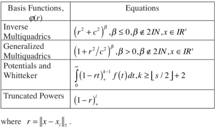
Table 2 shows strictly positive defi nite radial functions that are not Gaussian generalizations.

Table 2 Strictly positive defi nite radial functions not based on Gaussian function

Tablica 2 Striktno pozitivno defi nirane funkcije koje nisu temeljene na Gausovoj funkciji Basis Functions, j(r) Equations Inverse Multiquadrics r c IN x IR s 2₊ 2 _{0 2}

(

)

β,β≤ ,β∉ , ∈ Generalized Multiquadrics 1 0 2 2 2 +

(

r c

)

β _β> _β∉ IN x∈IRs , , , Potentials and Whitteker 1 1 2 2 0 −

(

)

+

( )

≥ ⎢⎣ ⎥⎦ + − ∞

∫

rt k f t dt k, s/ Truncated Powers

₍

_1−r

₎₊

l where r= x−xi 2.

4.3 Conditionally positive defi nite radial functions Another class of radial basis functions are conditionally posi-tive defi nite functions of order m, see Micchelli [1], and Guo at al. [19]. These are the functions that provide the natural generaliza-tion of RBF interpolageneraliza-tion with polynomial precision, important for high accuracy required for hull geometry description.

According to the theory of conditionally positive defi nite radial functions the RBF network defi nition can be changed to:

(10) where: p1pM form the basis for the M =

( )

_ms m+ −₋₁1 – dimensional

linear space Πm s

−1 of polynomials of total degree less than or equal

to m –1 in s variables.

There are conditionally and strictly conditionally positive defi nite functions. The condition for function F to be condition-ally positive defi nite is that it possesses a generalized Fourier transform of order m, continuous on IRs

0

{ }

, i.e. if Fˆ _is non-negative and non-vanishing.

To ensure unique solution M, additional conditions need to be added:

(11) with polynomial degree at most m – 1.

The function Fˆ _{is strictly conditionally positive defi nite} function of order m on IRS _{if its quadratic form is zero only for}

w≡0.

If their conditional positive defi niteness can be connected to complete monotone and multiple monotone functions and not generalized Fourier transform, we are obtaining the criteria for function F to be strictly conditionally positive defi nite radial function.

The examples of conditionally positive defi nite functions are shown in Fasshauer [13]:

− Generalized multiquadrics, Hardy [16],

− Thin plate splines (without shape parameter c, 2D polyhar-monic splines), see Duchon [20],

− Radial powers (without shape parameter c, 3D polyhar-monic splines), with no even powers.

Table 3 shows the list of some conditionally positive defi nite radial functions.

Table 3 Conditionally positive defi nite radial functions Tablica 3 Uvjetno pozitivno defi nirane radijalne funkcije

Functions j(r) Equations Generalized Multiquadrics 1 0 2 2 2 +

(

r c

)

β _β> _β∉ IN x∈IRs , , , Thin-plate spline

( )

− ∈ ∈ + 1β1_r2β _{rβ IN x IR}s log , , Radial Powers

( )

−1 >0 ∉2 ∈ β β_{r β β IN x IR}s , , ,

5 Polynomial precision

In general, solving interpolation problem with extended ex-pansion with polynomial term leads to solving a system of linear equations of the form:

(12) where H_ji = B_j(x_i), j, i = 1, …, N, P_jl = p_l(x_i), l = 1, …, M, w = [w₁, …, w_N]T_, ω _{= [}ω 1, …, ωM] T _{, y = [y} 1, …, yN] T _{and 0 is a zero} vector of length M.

The above system of linear equations can be solved using criterion (11) only, and therefore unique solution can be obtained by imposing this criterion.

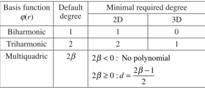
There is the minimal polynomial degree to be used depending on particular RBF selected [21] as shown in Table 4.

ˆ( ) , , f x wi x ti p x x IR i N l l l M s =

(

)

+

( )

∈ = =

∑

ϕ

∑

ω 1 1 w pi l i l M i N x

( )

= = =

∑

1 0, 1, , H P P w y 0 T 0 ⎡ ⎣ ⎢ ⎤_⎦⎥⎡_⎣⎢_ω⎤⎥ =_⎦ ⎡_⎣⎢ ⎤_⎦⎥

Table 4 The minimal degree of the polynomial depending on the RBF chosen

Tablica 4 Minimalni stupanj polinoma ovisno o odabranoj RBF Basis function

j(r)

Default degree

Minimal required degree

2D 3D Biharmonic 1 1 0 Triharmonic 2 2 1 Multiquadric 2β _{2 0} 2 0 2 1 2 β β β < ≥ = − : : No polynomial d

The goal of this paper is to select RBFs with high accuracy so polynomial precision is required. The RBFs having this prop-erty are acceptable only, and the basis functions will be selected among them.

6 Compactly supported radial basis

functions

Compactly supported RBFs are strictly conditionally posi-tive functions and radial of order m > 0, but not for all s on IRS_,

see Micchelli [1]. The acceptable range of compactly supported RBFs is defi ned for some restricted s range, with condition

s2 k m 2

⎢⎣ ⎥⎦ ≤ + − , i.e. maximal s value. This restriction ensures that F is integrable and therefore possesses classical Fourier transform F that is continuous. For integrable functions, the generalized Fourier transform coincides with the classical Fourier transform.

The compactly supported functions j s,k are all supported on

[0,1] and have polynomial representation there, with minimal degree for given space dimension s and smoothness 2k.

These functions j _s,k are strictly positive defi nite and radial on IRs _{and are of the form:}

(13) with a univariate polynomial j _s,k of degree _{⎢⎣ ⎥⎦ + +}s 2 3k 1.

In order to obtain compact support the distance between points needs to be divided by some value, d, that can be larger than points distance.

For example, the Wendland’s CSRBFs [3], are obtained from truncated power function ϕl

l

r

= −

(

1

)

₊ by dimension walk and repeatedly applied operator I, and we obtain: ϕs k ϕ

k

s k

I

, = _⎢⎣/2_{⎥⎦+ +}1.

Table 5 shows the list of some compactly supported functions, see Wendland [3], Wu [4], Buhmann [22].

The greatest advantage of CSRBFs is sparsing interpolation matrix H to some quasi-diagonal form, i.e. compact support en-sures that many elements of matrix H become zero. In that way, the inversion of interpolation matrix becomes easier, reducing quadratic matrix to some more computable one.

7 Global interpolation of 2D ship geometry

with radial basis functions

The conditionally positive defi nite and radial functions have polynomial precision when applied to scattered interpolation problem that is required for high accurate hull form geometry description.

When used in global interpolation those functions have global support. Globally supported functions chosen are:

− MQs,

− Inverse MQs,

− Generalized MQs,

− Thin-plate splines.

Additionally, compactly supported functions have polynomial representation on [0,1] and are suitable also for achieving high accuracy, and the functions to be used are:

− Wendland CSRBFs.

Therefore, the functions from Tables 3 and 4 are chosen for ship geometry modelling in this paper, with compact supported functions limited to Wendland’s functions for s = 3. Table 6 shows selected functions to be tested for accuracy in ship geometry description using RBF interpolation procedures.

Table 6 Testing radial basis functions

Tablica 6 Radijalne osnovne funkcije koje će se testirati Functions j(r) Equations MQ & Inverse MQ r c IN x IR s 2 2 2 +

(

)

β,β∉ , ∈ Generalized MQ

(

1_{+r c}2 2

)

β_,β>0_,β∉2_{IN x, ∈IR}s Thin-plate splines

( )

− ∈ ∈ + 1k1 2k s r log ,r k IN x, IR Wendland’s Compactly Supported RBFs ϕ ϕ ϕ 3 0 2 3 1 4 3 2 6 1 1 4 1 1 3 , , , = −

(

)

= −

(

)

[

+

]

= −

(

)

+ + + r r r r 55 2 18 3 r + r+ ⎡⎣ ⎤⎦

8 RBF parameters selection

The radial basis functions chosen have a few parameters depending on their type. Wendland’s CSRBFs have compact sup-ϕs k s k p r r r , , , , , , =

( )

∈

[ ]

> ⎧ ⎨ ⎪ ⎩⎪ 0 1 0 1

Table 5 Compactly supported functions Tablica 5 Funkcije s kompaktnom podrškom

Functions j(r) Equations Wendland _ϕ ϕ s l s r l s k r , , , / 0 1 1 2 1 1 = −

(

)

= ⎢⎣ ⎥⎦ + + = −

(

)

+ + with ll s l l r r l l r + + + +

(

)

+ ⎡⎣ ⎤⎦ = −

(

)

(

+ +

)

+ 1 2 2 2 2 1 1 1 4 3 3 ϕ, ⎡⎣

(

ll+6

)

r+3⎤⎦ Wu _ϕ ϕ s s r r r r r r , , 2 5 2 3 4 3 1 8 40 48 25 5 1 = +

(

)

(

+ + + +

)

= +

(

)

+ ++

(

+ + +

)

4 2 3 16 29r 20r 5r Buhmann Φ =12 4 −21 4+32 3−12 2+1 r logr r r r

port diameter d as parameter together with space dimension s and smoothness 2k. The rest of the functions have shape parameter c as parameter, together with the function exponent β.

8.1 MQRBFs

The MQRBFs are the functions described with one shape parameter c and exponent β value. Their high accuracy is re-quested in this paper, and therefore they are used together with polynomial term.

8.1.1 Exponent b values

The properties of multiquadric radial basis function can be clearly observed by graphical plot of Gamma and inverse Gamma function.

MQRBFs generalized Fourier transform has form for x_∈IRs

: (14) where: G is Gamma function, K_V is modifi ed Bessel function of the second kind of order v (MacDonald’s function), shape parameter c > 0and x is input variable.

Corresponding plot of Gamma and inverse Gamma func-tion is:

Figure 2 Gamma and inverse Gamma functions plot Slika 2 Graf Gama i inverzne Gama funkcije

If we observe the Gamma function in the denominator, its plot self-explanatory shows effi cient exponent b values to be used for MQRBFs, Figure 2. Obviously, integer bvalues should be avoided when using L₂ norm because of zero values.

8.1.2 Shape parameter c

The shape parameter c determines the shape of MQRBF cho-sen. The sensitivity diagram, Figure 3, shows the typical relations between shape parameter c and corresponding RMSE values.

It can be seen from the c – RMSE sensitivity diagram in Figure that the acceptable values of shape parameter c for high accuracy to be obtained are near zero value. Therefore, those values will be applied for MQRBFs in ship geometry description of 2D sections.

8.2 Wendland’s CSRBFs

The selection of different smoothness 2k, and the diameter of compact support are crucial for the representation properties of CSRBFs.

Corresponding compact support diameter is the parameter that quality of RBFs description mostly depends on and it will be varied in the results study in the next chapter

9 Results

The results of the RBF interpolation of the test section for the above chosen representative functions from Table 6 are extended with the polynomial of minimum degree. The accuracy of the description is checked on ship’s midship section with and without camber for chosen RBFs.

The RBF network quality of 2D ship section description will be observed for three corresponding description capabilities:

1. the description of form breaks,

2. the description of rounded form parts like the bilge, 3. the transition from rounded to fl at parts, like the transition from the bilge to the fl at of the side.

The break of the form between the deck and the side is checked against large oscillations characteristic for explicit in-terpolation procedures (“Gibbs phenomenon”) for general cargo ship test-section.

The quality of the representation of the rounded bilge part and its transition to the fl at of the side is checked on the main frame of one tanker with a fl at bottom, fl at sides and a rounded bilge with constant radius. This frame is chosen in order to check the quality and the accuracy of the RBF description of rounded geometry parts connected by the fl at of the side by 90 degrees.

9.1 Calculation accuracy

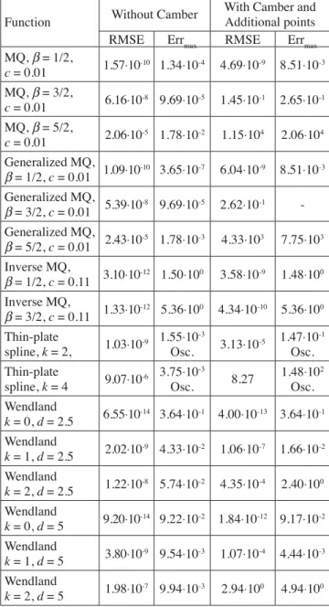
The results of RBF interpolation of the test sections for the ship geometry with and without camber are shown in Table 7 in order to observe RBF interpolation accuracy and quality of description of the ship’s test section.

ˆ _, Φ Γ ω β ω _{ω ω} β β β

( )

= −

( )

⎛⎝⎜ ⎞ ⎠⎟

(

)

≠ + − − + 2 0 1 ₂ 2 c K c s s

Figure 3 Sensitivity diagram c – RMSE

Table 7 RBF interpolation results of the ship’s test section Tablica 7 Rezultati RBF interpolacije brodskog rebra za provjeru

Function Without Camber

With Camber and Additional points RMSE Err_max RMSE Err_max MQ, β= 1/2, c = 0.01 1.57⋅10-10 1.34⋅10-4 4.69⋅10-9 8.51⋅10-3 MQ, β= 3/2, c = 0.01 6.16⋅10 -8 _9.69⋅10-5 _1.45⋅10-1 _2.65⋅10-1 MQ, β= 5/2, c = 0.01 2.06⋅10 -5 _1.78⋅10-2 _1.15⋅104 _2.06⋅104 Generalized MQ, β= 1/2, c = 0.01 1.09⋅10-10 3.65⋅10-7 6.04⋅10-9 8.51⋅10-3 Generalized MQ, β= 3/2, c = 0.01 5.39⋅10-8 9.69⋅10-5 2.62⋅10-1 -Generalized MQ, β= 5/2, c = 0.01 2.43⋅10 -5 _1.78⋅10-3 _4.33⋅103 _7.75⋅103 Inverse MQ, β= 1/2, c = 0.11 3.10⋅10 -12 _1.50⋅100 _3.58⋅10-9 _1.48⋅100 Inverse MQ, β= 3/2, c = 0.11 1.33⋅10-12 5.36⋅100 4.34⋅10-10 5.36⋅100 Thin-plate spline, k = 2, 1.03⋅10-9 1.55⋅10-3 Osc. 3.13⋅10-5 1.47⋅10-1 Osc. Thin-plate spline, k = 4 9.07⋅10 -6 3.75⋅10-3 Osc. 8.27 1.48⋅102 Osc. Wendland k = 0, d = 2.5 6.55⋅10 -14 _3.64⋅10-1 _4.00⋅10-13 _3.64⋅10-1 Wendland k = 1, d = 2.5 2.02⋅10-9 4.33⋅10-2 1.06⋅10-7 1.66⋅10-2 Wendland k = 2, d = 2.5 1.22⋅10-8 5.74⋅10-2 4.35⋅10-4 2.40⋅100 Wendland k = 0, d = 5 9.20⋅10 -14 _9.22⋅10-2 _1.84⋅10-12 _9.17⋅10-2 Wendland k = 1, d = 5 3.80⋅10-9 9.54⋅10-3 1.07⋅10-4 4.44⋅10-3 Wendland k = 2, d = 5 1.98⋅10-7 9.94⋅10-3 2.94⋅100 4.94⋅100 (Note: “Osc.” marks large bottom end oscillations)

The acceptable values of global and local representation are obtained for the test-section without camber only, with MQRBF and generalized MQRBF with β= 3/2 giving acceptable val-ues.

The results for the section with camber do not have required Err_max accuracy, with Wendland’s CSRBF with s = 2, k = 1 and d = 5 having results the closest to the required ones. After the diameter d is set to 6.8, better values are obtained: RMSE = 5.0_⋅10-4 _{and Err}

max = 9.66⋅10

-4_{, showing CSRBFs dependency}

on that parameter.

It has to be noted, that MQRBFs with β= 1/2 and Wendland’s function with k = 0 give straight lines of the description with C0

continuity, and therefore they can be neglected.

9.2 Section without camber

The results for the section without camber are acceptable for almost all RBF choices except thin-plate spline that oscillates near the bottom.

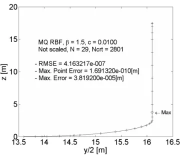
Figure 4 shows the acceptable MQRBF representation of the test-section with β = 1.5, and with Ncrt number of drawing points.

Figure 4 The result of the MQRBF generalization of the ship test-section with b = 3/2, c = 0.01

Slika 4 Rezultat poopćavanja brodskog test-rebra pomoću MQRBF sa b = 3/2, c = 0,01

The oscillations of the description at the transition from the rounded bilge to the fl at side are shown in Figure 5.

Figure 5 The zoom of MQRBF generalization of the ship test-sec-tion with b = 3/2, c = 0.01

Slika 5 Povećanje MQRBF poopćenja brodskog test-rebra sa b = 3/2, c = 0,01

Figure 5 is Figure 4 zoom, and it shows slight oscillations near the curves transition from the rounded bilge to the straight side, as shown in Figure 5, of order 10-4 _{that can be taken as acceptable}

value. The additional points around transition can straighten the RBF curve in the fl at part, this enabling required transition. 9.3 Section with camber

For the RBF description of the section with camber, the break of the form is the problem that cannot be solved acceptably for all chosen functions.

Because of large oscillations of RBF descriptions at the upper section end, at shear strike, a single point is added very near it to stabilize the generalization curve at the distance 10-4 _{from the}

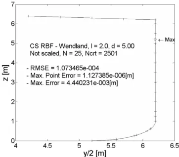
top at the side. After stabilization, the only accurate and smooth functions are Wendland’s functions with k = 1, s = 2 and d = 5, with a slightly lower local accuracy Err_max than required, as shown in Figure 6.

Figure 6 Wendland’s CSRBF generalization of the ship’s test-sec-tion with camber

Slika 6 Poopćavanje brodskog test-rebra s prelukom Wendlan-dovom CSRBF

In order to adequately describe curved and fl at parts of the section, additional points are added, thus showing the need for adjustments in RBF description. The advantage of these adjust-ments is in the fact that the required accuracy is easy to achieve, and a small number of added points is needed for high quality of description, thus showing fl exibility of RBF representation. 9.4 Description of the rounded bilge with transition to

the fl at of the side

The RBFs capability of rounded parts description, with some radius, is observed in the description of the midship section of the test tanker with transition to the fl at of the side.

The bilge is described in two ways:

− with standard point distribution, and

− with Chebyshev points.

When described with standard point distribution, the section bilge is described on “standard” height point positions: 0, 0.01, 0.025, 0.100, 0.250, 0.500, 0.75, 1.000, 1.250, 1.500, 1.750, 2.000, 2.250, 2.500 metres. The rest of the section is described with equally distributed heights on the side and with equally dis-tributed points on the bottom with some appropriate distance.

After calculations are made for chosen RBFs, the results are acceptable for standard shipbuilding point distribution only, and not for Chebyshev points. In mathematical sense, that means when the points are regular they will produce poor representation, with unexpected oscillations on the curved and fl at parts for the description of the bilge transition to the fl at of the side.

Moreover, the results are tolerant for MQRBFs only, show-ing the problems with compactly supported RBFs when applied in global context.

Figure 7 shows the MQRBF descriptions of the tanker test-section, without camber, and standard point distribution of the bilge.

Figure 7 Bilge and bilge transition description with MQRBF de-scribed by standard point distribution

Slika 7 Uzvoj i prijelaz s uzvoja na ravni bok opisan pomoću MQRBF sa standardnim rasporedom točaka

It can be seen from Figure 7 that the quality of description is not good enough, with low Err_max value. Two additional points are added to improve the section description, on heights: 0.041 and 2.493, as shown in Figures 8 and 9 below.

After that, the representation has improved to required Err_max and RMSE values with better quality of the circle arc description of the bilge.

It can be seen that the RBF description of conic sections depends on the number and position of the input points and is not natural property like in NURB splines. The required accuracy cannot be obtained in the curved part of the section with the transition to straight parts, without local adjustments of shape parameter c. So, in order to obtain a higher accuracy, parameter c should be changed from global to local parameter, but that is out of the scope of this paper.

Once the required accuracy is obtained, scaling can be used to transform the RBF description to the actual bilge radius.

Figure 8 Bilge and bilge transition description with MQRBF de-scribed by standard point distribution and additional two points

Slika 8 Opis uzvoja i prijelaza na ravni bok opisan MQRBF sa standardnim točkama i dvije dodatne točke

10 Example of RBF representations of other

ship frame

The above presented examples of frame description are fo-cused to the accuracy of the description of some rounded bilge and to the transition to the fl at of the side. The following example of frame description will show RBF description capabilities of

Figure 9 Bilge zoom description, with MQRBF and 2 additional points added, and the discrepancy from ideal bilge circle arc by the bilge curve length

Slika 9 Uvećani uzvoj, opisan sa MQRBF sa 2 dodane točke, s odstupanjem od idealnog luka kružnice po duljini krivulje uzvoja

Figure 10 MQRBF generalization with b = 3/2, c = 0.001 of multiple curved aft frame with camber and bulb

Slika 10 Opis višestruko zakrivljenog krmenog rebra sa prelukom i bulbom MQRBF poopćenjem sa b = 3/2 c = 0,001

multiply curved frame with camber. Figure 10 shows RBF de-scription of the aft frame of the general cargo test ship with high curvature, bulb and camber.

This example shows the capability of RBF networks in very accurate global description of multiple curved frames with camber, and therefore it can be assumed that RBF networks are suitable for 2D ship frames description.

11 Conclusion

The RBF interpolation is applicable in 2D ship geometry description, extended with polynomial terms of minimal degree, when conditionally positive defi nite radial functions are used.

The high accuracy required can be obtained by input point data set adjustment, with less effort needed than in spline based methods. The transition from the rounded bilge to the fl at of the side is comparable to NURB and B-splines, with possible adjust-ments using added points in order to achieve required smoothness of the rounded part, and fl atness of the straight part of the section. The same can be concluded for the description of knuckles where the adjustment of input data set must be performed, too.

The bijection problems overall can be solved by geometric transformations, satisfying C continuity requirements.

Overall conclusion is that RBF interpolation procedures are comparable to those based on B-splines and NURB splines, and the effort should be done to further improve RBF representation of straight and rounded parts and to extend this work to corre-sponding 3D representations of the hull form.

References

[1] MICCHELLI, C. A.: “Interpolation of scattered data: Dis-tance matrices and conditionally positive defi nite functions”, Constr. Approx. 2, p. 11-22, 1986.

[2] SCHABACK, R.: “Creating surfaces from scattered data using radial basis functions”, in “Mathematical Methods for Curves and Surfaces”, (M. Dæhlen et al. eds.), Vanderbilt University Press, p. 477-496, 1995.

[3] WENDLAND, H.: “Piecewise polynomial, positive defi -nite and compactly supported radial functions of minimal degree”, Adv. in Comput. Math. 4, p. 389-396, 1995. [4] WU, Z.: “Compactly supported positive defi nite radial

functions”, Adv. in Comput. Math., p. 283-292, 1995. [5] BOCHNER, S.: “Monotone Funktionen, Stieltjes Integrale un

Harmonische Analyise”, Math. Ann. 108, p. 378-410, 1933.

[6] SCHOENBERG, I.J.: “Metric spaces and completely mono-tone functions”, Ann. of Math. 39, p. 811-841, 1938. [7] SCHOENBERG, I.J.: “Metric spaces and positive defi nite

functions”, Trans. Amer. Math. Soc. 44, p. 522-536, 1938. [8] ARONSZAJN, N.: “Theory of reproducing kernels”, Trans.

Amer. Math. Soc. 68, p. 337-404, 1950.

[9] MATHIAS, M.: “Über positive Fourier-Integrale”, Math. Zeit. 16, p. 103-125, 1923.

[10] STEWART, J.: “Positive defi nite functions and generaliza-tions, an historical survey”, R. M. J. Math 6, p. 409-434, 1976.

[11] WENDLAND, H.: “Scattered Data Approximation”, Cam-bridge University Press (CamCam-bridge), 2005.

[12] WILLIAMSON, R. E.: “Multiple monotone functions and their Laplace transform”, Duke Math. J. 23, p. 189-207, 1956.

[13] FASSHAUER, G. E.: “Meshfree Approximation Methods with Matlab”, Interdisciplinary Mathematical Sciences – Vol. 6, World Scientifi c Publishing Co. Pte. Ltd., 2007. [14] ANDREWS, G. E., ASKEY, R., ROY, R.: “Special

Func-tions”, Cambridge University Press, 1999.

[15] FORNBERG, B., LARSON, E., WRIGHT, G.: “A new class of oscillatory radial basis functions”, Com. Math. App. 51, p. 1209-1222, 2004.

[16] HARDY, R. L.: “Multiquadric equations to topography and other irregular surfaces”, J. Geophys. Res. 76, p. 1905-1915, 1971.

[17] FORNBERG, B., WRIGHT, G.: “Stable computation of multiquadric interpolants for all values of shape parameter”, Comp. Math. Appl. 47, p. 497-523, 2004.

[18] ABRAMOWITZ, M., STEGUN, I. A.: “Handbook of Math-ematical Functions with Formulas, Graphs, and Mathemati-cal Tables”, Dover (New York), 1972.

[19] GUO K. at al.: “Conditionally positive defi nite functions and Laplace-Stieltjes integrals”, J. Appr. Th. 74, p. 249-265, 1993.

[20] DUCHON. J.: “Interpolation des fonctions de deux variables suivant le principle de la fl exion des plaques minces”, Rev. Franc. Autom. Inf. Rech. Oper. Anal. Numer. 10, p. 5-12, 1976.

[21] …: FastRBF Toolbox, Matlab Interface Version 1.4., Far-Field Technology, 2004.

[22] BUHMANN, M. D.: “Radial functions on compact support”, Proc. Edin. Math. Soc. II 41, p. 33-46, 1998.