Jakub Gajarský
Technical University Berlin, Germany [email protected]
Stephan Kreutzer
Technical University Berlin, Germany [email protected]
Abstract
Shrub-depth is a width measure of graphs which, roughly speaking, corresponds to the smallest depth of a tree into which a graph can be encoded. It can be thought of as a low-depth variant of clique-width (or rank-width), similarly as treedepth is a low-depth variant of treewidth. We present an fpt algorithm for computing decompositions of graphs of bounded shrub-depth. To the best of our knowledge, this is the first algorithm which computes the decomposition directly, without use of rank-width decompositions and FO or MSO logic.
2012 ACM Subject Classification Theory of computation→Fixed parameter tractability; Math-ematics of computing→Combinatorial algorithms
Keywords and phrases shrub-depth, tree-model, decomposition, fixed-parameter tractability
Digital Object Identifier 10.4230/LIPIcs.STACS.2020.56
Funding The research is supported by the European Research Council (ERC) under the European Union’s Horizon 2020 research and innovation programme (ERC consolidator grant DISTRUCT, agreement No. 648527).
Acknowledgements We want to thank Sang-il Oum for suggesting that our techniques may be used to obtain the results of Section 6.
1
Introduction
Among the numerous width parameters used in graph theory and algorithmics, treewidth and its dense counterparts clique-width and rank width are arguably the most prominent and extensively studied. In recent years, more restrictive parameters, which could be collectively called depth parameters, are attracting increasing attention. The best-known of these is treedepth [10], which can be seen as a low-depth variant of treewidth. Inspired by the usefulness of treedepth, the authors of [8] defined the notion of shrub-depth, which can be seen as a low-depth variant of clique-width, analogously to the relation between treedepth and treewidth.
Since shrub-depth is a more restrictive notion than clique-width, it is natural to ask what algorithmic advantages it offers over clique-width, if any. The question whether some problems which are parameterized intractable on graphs of bounded clique-width are fixed-parameter tractable on graphs of bounded shrub-depth was addressed in [7], where it was shown that the Hamiltonian path and the chromatic number problem remain hard on graph classes of bounded shrub-depth. On the other hand, bounded shrub-depth offers certain quantitative advantages over clique-width. For instance, a well-known result of Courcelle, Makowski and Rotics [2] states that every MSO definable propertyϕof graphs can be solved in time f(ϕ)· |V(G)| on any class of graphs of bounded clique-width. The price for the generality of this result is that the functionf is non-elementary, i.e. it grows like a tower of exponentials whose height depends on the formula. But as shown in [5], on any graph class shrub-depthdthe function f is only d-fold exponential, i.e. its height does not depend on the formula.
Besides being interesting in their own right, shrub-depth has important consequences for much more general graph classes. To explain this, we will first describe the analogous situation in the case of sparse graphs and treedepth. Nešetřil and Ossona de Mendez introduced [11] the notions of bounded expansion and nowhere denseness as a general approach to studying sparse graphs in a unified setting. Graphs from classes of bounded expansion and nowhere dense graph classes can be decomposed1 into several overlapping graphs each of small treedepth. Such a decomposition has successfully been used for solving many problems on graph classes of bounded expansion and nowhere dense graph classes efficiently. In some cases, the problems can be reduced to solving them on the graphs of small treedepth obtained by this decomposition, and in more complicated cases one can repeatedly perform computations on graphs of small treedepth from the decomposition and then combine the results.
Recently a dense counterpart of the notion of bounded expansion has been studied under the namestructurally bounded expansion, and the results of [6] indicate that shrub-depth could play a role analogous to treedepth in the sparse case: it was shown that every graph from a class of graphs of structurally bounded expansion can be decomposed into a bounded number of subgraphs of small shrub-depth and this decomposition can then be used for algorithmic purposes. Given this promising application of shrub-depth in the theory of dense but structurally simple graphs, it is very likely that a better structural understanding of shrub-depth will be of increasing relevance in the near future.
All width and depth measures mentioned so far are defined by an associated concept of decomposition. For shrub-depth this decomposition is called atree-model. Unlike other width measures, tree-models are defined in terms of two parameters, commonly denoted byd
andm. To use any of the mentioned depth or width measures algorithmically, one usually needs to be able to compute the corresponding types of decompositions for an input graph
G. In most cases, the problem of finding an optimal decomposition of an input graph is NP-hard, but often for fixed values of the relevant width parameters one can, in polynomial time, either find a decomposition with the prescribed value or correctly decide that no such decomposition exists. This is the case for treewidth [1], rank-width [9] and treedepth [12]. Algorithms like this are calledparameterized algorithmsand are studied in the framework of parameterized complexity theory. We refer to [3] for an indepth introduction to parameterized complexity and only briefly recall the concepts from parameterized complexity needed below. Aparameterized problem P is essentially a classical problem but in addition to the normal input instancewwe are given an integerk, the so-calledparameter. The problemP is called fixed-parameter tractable, or in the complexity class FPT, if there is a computable functionf
and a constantcsuch that the problem can be solved by an algorithm whose running time on input (w, k) is bounded byf(k)· |w|c. The class FPT can be seen as the parameterized equivalent to the classical complexity classP as abstraction of efficiently solvable problems.
A much weaker requirement on the running time is imposed by the parameterized complexity class XP. The problem P is in XP if there is a computable function f such that the problem can be solved by an algorithm whose running time is bounded by|G|f(k). Thus, a problem is in XP if it can be solved in polynomial time for every fixed value of the parameterk.
Our contribution. We provide combinatorial and conceptually simple algorithms for
com-puting tree-models with given parameters d and m of input graphs G. To obtain our algorithms, in Section 3 and 4, we introduce a new concept ofk-modules and prove several
1 The precise meaning of this is rather technical and is not important for our purpose, so we omit the precise definition.
properties relatingk-modules and tree-models of graphs. The structural results we obtain provide a new and very different insight into the structure of graphs of low shrub-depth which we believe will be of further interest. These results provide the basis for our algorithms for computing tree-models, which we present in Section 5. Our main algorithmic result is an fpt-algorithm for computing tree-models with prescribed parametersdandm in a graphG, providedGhas such a model. Finally, in Section 6, we present another application of our results to forbidden induced subgraphs of graph classes of bounded shrub-depth.
Previous work. To the best of our knowledge, no papers explicitly address the problem of
computing tree-models with given parameters dandmof a given input graph. However, there exists a folklore fpt algorithm for computing an optimal SC-decomposition of a given graph, where SC-decomposition is a notion closely related to tree-model. This algorithm requires computing a rank decomposition of the input graphGfirst and then uses a powerful algorithmic metatheorem for MSO logic to obtain the SC-decomposition. Similarly, the results and techniques of [5] can likely be adjusted to compute tree-models, but also in this case one would have to rely on computing a rank decomposition first and using a logical metatheorem.
2
Preliminaries
For n ∈ N we denote the set {1, . . . , n} by [n]. For sets A, B we denote by A∆B their symmetric difference (A\B)∪(B\A).
Graphs. All graphs in this paper are finite, undirected and simple. We use standard graph
theoretic notation, see e.g. [4]. Let Gbe a graph. If X ⊆V(G) we denote by G[X] the subgraph ofGinduced byX and byG−X the subgraph induced byV \X. IfX={v}is a singleton set, we simply writeG−v for G− {v}. We denote by NG(v) the neighbourhood of v ∈V(G) in G. If Gis understood we omit the index and just write N(v). Let G, H
be graphs and let λ : V(G) → [m] and λ0 : V(H) → [m] be labelling functions. A label preserving isomorphism between (G, λ) and (H, λ0) is a bijective functionf :V(G)→V(H) such that {u, v} ∈ E(G) if, and only if, {f(u), f(v)} ∈ E(H) and λ0(f(v)) =λ(v) for all
u, v∈V(G).
Trees. By a tree in this paper we mean a rooted connected acyclic graph. LetT be a tree
with rootr. TheancestorsoftinT are the vertices on the unique path fromrtotinT other thantitself. Theparent oftis the ancestor oftadjacent tot. The rootritself does not have a parent. Fort∈V(T)\ {r} we define thesubtree Ttof T rooted at tas the component of
T−econtainingt, whereeis the edge incident to tand its parent. Fort=rwe setTr=T. Thechildren oft are the neighbours oftother than the parent. Thedescendants oft are the vertices inV(Tt)\ {t}.
A leaf ofT is a node of degree 1 which is not the root. We denote the set of leaves ofT
byleaves(T). Nodess, t∈V(T) arecomparable (inT) ift∈V(Ts) ors∈V(Tt). Otherwise they areincomparable. Theheight of tis the maximal length of a path fromtto a leaf of
Tt. Given a setX ⊆V(T) we define theleast common ancestor ofX, denoted bylca(X), as the nodet∈V(T) of minimal height such that X⊆V(Tt). We also writelca(u1, . . . , ut) for
lca({u1, . . . , ut}). Thedistancebetween two nodess, t∈V(T), denoted by distT(s, t), is the length of the unique path betweensandtinT.
Shrub-depth. Shrub-depth was defined by Ganian et al. in [8]. It is defined using the following notion oftree-model.
IDefinition 2.1. Letdandmbe non-negative integers and letGbe a graph. Atree-modelof
Gis a triple(T, S, λ), whereT is a tree,S⊆[m]2×[d]is a relation, andλ:leaves(T)→[m] is a function, such that
i. the length of each root-to-leaf path is exactlyd,
ii. the set leaves(T)of leaves is exactlyV(G),
iii. (i, j, d)∈S if, and only, if (j, i, d)∈S (symmetry in the colours), and
iv. for any two vertices u, v ∈ V(G), if λ(v) = i, λ(v) = j and distT(u, v) = 2l, then
{u, v} ∈E(G)if, and only if, (i, j, l)∈S.
Note that the leaves leaves(T) of T are the vertices of G. Thus, if v ∈ V(G), then
v∈leaves(T) and thereforeλ(t) is defined. The numberdin the above definition is referred to as the depth of the tree-model. We will often speak of a (d, m)-tree-model instead of a “tree-model of depthdwithmcolours”.
Note that every graphGhas a tree-model of depth 1 with |V(G)|colours (each vertex gets its own colour and the relationS is essentiallyE(G)). Thus it does not make sense to ask about the smallest depth of a tree-model of a graphG. This is the reason why the notion ofshrub-depth is defined only for classes of graphs.
IDefinition 2.2. The shrub-depthof a graph classC is the smallest d >0 for which there
exists an m >0 such that every graphG∈ C has a (d, m)-tree-model.
We remark that even though the shrub-depth of a graph classC is defined as one number (din the above definition), to each class C of graphs of bounded shrub-depth there actually correspond two numbers –dandm from the above definition. Thus, in what follows, we usually work directly with (classes of) graphs which have a (d, m)-tree-model for some fixed
dandm.
IDefinition 2.3. LetGbe a graph and G0⊆Gbe an induced subgraph ofG. Letd, m >0.
A (d, m)-tree-model (T, S, λ) of G extends a(d, m)-tree-model (T0, S0, λ0) of G0 if T0 ⊆T,
S=S0 andλ(v) =λ0(v)for allv∈V(G0).
We frequently use the following result from [8] which follows immediately from the definition of shrub-depth: if (T, S, λ) is a (d, m)-tree-model ofG, then we can obtain a (d, m )-tree-model (T0, S0, λ0) ofG0 as follows: the treeT0 is the minimal subtree ofT containing the root ofT and all leaves formV(G0). Similarly,λ0 is the restriction of λtoV(G0) and
S0=S. In particular, the tree-structure ofT is preserved in the reduced tree-modelT0.
IProposition 2.4 ([8]). Let d, m >0. If Ghas a (d, m)-tree-model and G0 is an induced
subgraph ofG, thenG0 also has a (d, m)-tree-model.
3
Twin tuples,
k
-modules and outline of our approach
In this section we introduce the concepts oftwin tuples and(strict)k-moduleswhich will be pivotal in the rest of the paper and briefly outline the key idea behind our algorithm for finding a (d, m)-tree-model of an input graphG.
3.1
Twin tuples and (strict)
k
-modules
I Definition 3.1. Let k ∈ N and let G be a graph. Two disjoint tuples (a1, . . . , ak),
(b1, . . . , bk)∈V(G)k are twin tuplesif
1. the function f(ai) = bi, 1 ≤ i ≤ k, is an isomorphism between G[{a1, . . . , ak}] and
G[{b1, . . . , bk}],
2. {ai, bj} ∈E(G) if, and only if,{aj, bi} ∈E(G), for all1≤i < j≤k, and
3. N(ai)\ {a1, . . . , ak, b1, . . . , bk}=N(bi)\ {a1, . . . , ak, b1, . . . , bk} for all 1≤i≤k.
Fork= 1we simply call a1 andb1 twins. A set M of pairwise disjoint k-tuples of vertices ofG is astructured k-moduleif all tuples inM are pairwise twin tuples.
The next definition introduces a different characterisation of k-modules which we will use frequently in the sequel. The equivalence between the two definitions is easily seen (and stated formally in the lemma thereafter).
IDefinition 3.2. Letk∈Nand letα, β be symmetric relations on [k]2. Let Gbe a graph.
A set M ⊆V(G)k of pairwise disjoint k-tuples is an (α, β)–module if
1. for every (a1, . . . , ak)∈M,{ai, aj} ∈E(G)if, and only, if (i, j)∈α,
2. for all distinct tuplesa1, . . . , ak, b1, . . . , bk ∈M, {ai, bj} ∈E(G)if, and only, if(i, j)∈β,
and
3. N(ai)\S = N(bi)\S for all 1 ≤i ≤ k and all (a1, . . . , ak),(b1, . . . , bk)∈ M, where
S :=S{a
i : 1≤i≤k,(a1, . . . , ak)∈M}.
We callk-tuples ¯a,¯b∈V(G)k (α, β)-twins, if{a,¯ ¯b} is an (α, β)-module inG.
ILemma 3.3. A setM of pairwise distinct k-tuples is a structuredk-module if, and only if,
there are symmetric relationsα, β on[k]2 such that M is an (α, β)-module.
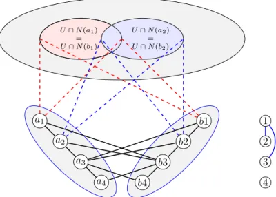
Thus, in a structured k-module M, the relationαdetermines the adjacency within each tuple ¯a∈M, or the isomorphism type of the subgraphs ofGinduced by the tuples in the module and the relationβfixes the adjacency between different tuples fromM. Furthermore, any two vertices at the same position within their respective tuples have the same adjacency to the vertices outside the module. The notion ofk-module is illustrated on Figure 1.
Givenα, βas above, we say that the structuredk-moduleM isdetermined orinducedby
α, β. Also, if ¯aand ¯b are twin tuples such that the adjacency within ¯aand ¯band between ¯a
and ¯bis determined by relationsαandβ, we say that ¯aand ¯bare (α, β)-twin tuples. The following simple fact will be used often in the sequel.
ILemma 3.4. Let ¯a,¯b,c¯∈V(G)k be tuples such thata¯ is an(α, β)-twin tuple of¯b and¯b is an(α, β)-twin tuple ofc¯. Thena¯ is an (α, β)-twin tuple ofc¯. In other words, for any fixedα
andβ the relation of being(α, β)-twin tuples is transitive.
The next lemma captures the intuition behindk-modules and their connection to tree-models.
I Lemma 3.5. Let (T, S, λ) be a tree-model of a graph G and let u ∈ V(T) be a node
withL≥2children{1, . . . , L} such that for any pairi, j of its children there exists a label preserving isomorphismιij betweenTi andTj. ThenGcontains ak-module withL tuples,
wherek=|leaves(T1)|.
Proof. Fix an ordering ≤1 on leaves(T1). Then, for every j >1, we define an order ≤j on leaves(Tj) as follows: u ≤j v, for u, v ∈ leaves(T1), if, and only if, ιj1(u) ≤1 ιj1(v). Each pair (leaves(Ti),≤i) can be thought of as a k-tuple, and it is easy to see thatM :=
{(leaves(T1 ),≤1), . . . ,(leaves(TL),≤L)} is a k-module with L tuples as claimed in the
a1 a2 a3 a4 b4 b3 b2 b1 1 2 3 4 U∩N(a1) = U∩N(b1) U∩N(a2) = U∩N(b2)
Figure 1 An example of a 4-module M with two tuples (a1, a2, a3, a4) and (b1, b2, b3, b4). The set U is V(G) \ {a1, a2, a3, a4, b1, b2, b3, b4}. Relations α and β are defined as follows: α={(1,2),(2,1),(2,3),(3,2),(3,4),(4,3)},β={(1,3),(3,1),(2,3),(3,2),(3,4),(4,3)}. The conflict graph ofM (Definition 3.7) is on the right. Note thatM0={(a1, a2, a3)(b1, b2, b3)}is also a module, and since its conflict graph (only on vertices 1,2,3) is connected, it is an example of a strict module (Definition 3.8).
3.2
Outline of our approach
We now present an outline of our approach for computing tree-models. By Lemma 3.5, if a tree-model of a graphGcontains several isomorphic subtrees with common parent, then these subtrees induce ak-module inG. If the converse statement
(∗) if ¯a, ¯b, ¯c, . . . ,form a moduleM ofG, then in every tree-modelT ofGthe vertices of tuples ¯a,¯b,¯c, . . .are the leaves of distinct but isomorphic subtreesTa, Tb, Tc, . . . with a common parent u
was also true, then this could be used to compute tree-models as follows: compute a module
M ={¯a,¯b,c¯}in the input graphGand remove ¯cfromGto obtainG0with moduleM0={¯a,¯b}. Then it would be enough to find any(d, m)-tree-modelT0 ofG0 which then can easily be extended to a tree-modelT ofG– by (∗) the tree-model T0 contains different isomorphic subtreesTa andTb (representing ¯aand ¯b) with a common parentu, and so we can create a copyTc of Ta and add it as a child of uto create a tree-modelT of G. This essentially means that by finding a moduleM inGwe can, by deleting a tuple fromM, reduce the problem of computing a tree-model with parametersdandmofGto a problem of finding a tree-modelT0 with the same parameters but for a smaller graphG0.
We will essentially follow this idea but use a weaker statement than (∗) instead. It turns out that even less than having isomorphic subtrees is enough to make the above idea work – it is enough to have a tree-modelT0ofG0 in which two tuples ¯aand ¯bare in a “good position” with respect to each other, as shown in the following lemma, proved below, which is the basis of our approach.
ILemma 3.6. LetGbe a graph and let{(a1, . . . , ak),(b1, . . . , bk),(c1, . . . , ck)}be ak-module
in G. Let G0 =G− {c1, . . . , ck} and let (T0, S0, λ0) be a(d, m)-tree-model of G0, for some
1. lca({a1, . . . , ak})and lca({b1, . . . , bk}) are incomparable inT0 and
2. for all i∈[k] the labelsλ0(ai)andλ0(bi)are the same in T0.
Then(T0, S0, λ0)can be extended to a (d, m)-tree-model(T, S, λ)ofG.
Unfortunately, the statement (∗) does not hold and neither does the following weaker statement (∗∗) which would still be strong enough for our purpose: ifM is ak-module in a graphG, then in any tree modelT ofGthere are at least two tuples (a1, . . . , ak),(b1, . . . , bk)∈
M which satisfy the requirements of Lemma 3.6 with respect to T. In general, if ¯aand ¯b
are twin tuples of graph G, the vertices (a1, . . . , ak) and (b1, . . . , bk) can be placed almost arbitrarily “badly” in a tree-modelT ofG. In order to be able prove a variant of (∗∗), we will have to restrict ourselves to a more structured notion of module, which we call astrict module. Strict modules are modules in which the vertices in each tuple are forced to “stick together” – we want to avoid the situation when it is possible to exchangeai forbi between two tuples (a1, . . . , ak) and (b1, . . . , bk) without violating αor β. More generally, we want it to be impossible for any non-empty subsetIof [k] to exchange{ai}i∈I for{bi}i∈I between two tuples (a1, . . . , ak) and (b1, . . . , bk) without violatingαandβ. This will be accomplished using the notions ofconflict andconflict graph.
IDefinition 3.7. LetM be ak-module of a graphGinduced by relations α, β. We say that
positions i, j ∈[k] with i6=j are in conflict if(i, j)∈α but (i, j)6∈β or vice versa. The conflict graphC(M) of M is the graph with vertex set[k] and an edge betweeni and j if, and only if, the positions iandj are in conflict.
IDefinition 3.8. An(α, β)-moduleM is a strictk-moduleif its conflict graph is connected.
The definition of strict k-modules will allow us to prove Lemma 4.1, which can be seen as a variant of (∗∗). Informally it says that ifGis a graph with a large strictk-moduleM, then in any (d, m)-tree-model T ofGthere are two tuples in a “good” mutual position in T
(i.e. in the position required in Lemma 3.6). With Lemma 4.1 at hand, it remains to bound the valuek in terms ofdand mand to show that sufficiently large strictk-modules always exist in graphs which have (d, m)-tree-models (Corollary 4.6). Finally, we need to design algorithms for computing large strictk-modules in an input graphG(Section 5).
We close this section by proving Lemma 3.6 and a corollary, which will be used in Section 5.
Proof of Lemma 3.6. Let va, vb be the least common ancestors of {a1, . . . , ak} and
{b1, . . . , bk}, resp., and letv=lca(va, vb). LetTa be the minimal subtree ofTv containing
va and{a1, . . . , ak}. Thus,Ta has exactlykleavesa1, . . . , ak. LetTd be an isomorphic copy ofTa. Letd1, . . . , dk be the leaves ofTd such thatdi is the copy ofai, for all 1≤i≤k.
Let T be the tree obtained fromT0∪Td by identifying the root ofTd with v, i.e.T is the treeT0∪S1∪. . .∪Sl plus the edges{v, si}, for 1≤i≤l, whereS1, . . . , Sl are the subtrees ofTd rooted at the childrens1, . . . , slof the root ofTd. We setS=S0 and define a labelling functionλon the leaves of T by settingλ(t) =λ0(t), ift6∈ {d1, . . . , dk}andλ(di) =λ0(ai). Then (T, S, λ) is a tree-model of the same height as (T0, S0, λ0) using the same set of labels.
It remains to verify that the graphGT defined byT is isomorphic toG. By construction,
V(GT) =V(G)\ {c1, . . . , ck} ∪ {d1, . . . , dk}. Let π:V(GT)→V(G) be the function with
π(u) =ufor all u∈V(G)\ {d1, . . . , dk} andπ(di) =ci, for 1≤i≤k. We claim that πis an isomorphism betweenGT andG.
Asπis bijective by construction, it suffices to show that{u, w} ∈E(GT) if, and only if, {π(u), π(w)} ∈E(G). Ifu, w∈V(G)\ {c1, . . . , ck}there is nothing to show as the adjacency of all vertices withinG0=G− {c1, . . . , ck} remains unchanged by attachingS1, . . . , Sl toT0. Now suppose u= di and w =dj, for some 1 ≤i =6 j ≤ k. Then λ(di) = λ(ai) and
λ(dj) =λ(aj) and the distance 2lbetweendianddjinT is the same as the distance between
ai andaj. Thus
{di, dj} ∈E(GT)⇔(λ(di), λ(dj), l)∈S⇔ {ai, aj} ∈E(GT)⇔ {ai, aj} ∈E(G), as argued above. As{{a1, . . . , ak},{c1, . . . , ck}}is ak-module inG, {ci, cj} ∈E(G) if, and only if,{ai, aj} ∈E(G). Thus, the restriction ofπto{d1, . . . , dk}is an isomorphism between the subgraphsG[{c1, . . . , ck}] andGT[{d1, . . . , dk}].
The last case to consider is when u = di, for some 1≤ i ≤k, and w 6∈ {d1, . . . , dk}. Suppose first thatw6∈V(Tv), wherev=lca(va, vb). Then the distance betweenwandai in
T is the same as between wanddiand therefore
{di, w} ∈E(GT)⇔ {ai, w} ∈E(GT)⇔ {ai, w} ∈E(G)⇔ {ci, w} ∈E(G).
Finally, suppose w∈V(Tv). In this case either the path betweenw andui containsv and therefore the distance betweenwandui is the same as the distance betweenwandai, or the path betweenwandui does not containv and the distance between wandui is the same as the distance betweenwandbi. As the adjacency betweenw, ai, w, bi andw, ci is the same inG, this implies that{w, di} ∈E(G) if, and only if, {w, ci} ∈E(G). J
The next result follows easily by induction on|M \ {¯a,¯b}|using Lemma 3.6.
ICorollary 3.9. Let d≥0and k, m ≥1. Let Gbe a graph and let M be a k-module in
G. Let ¯a,¯b ∈M and let G0 =G−S
{c¯: ¯c ∈M \ {¯a,¯b}}. If there is a (d, m)-tree-model (T0, S0, λ0) of G0 such that lca({a1, . . . , ak}) and lca({b1, . . . , bk}) are incomparable in T0
and λ0(ai) = λ0(bi) for alli ∈[k], then G has a(d, m)-tree-model (T, S, λ) which extends (T0, S0, λ0).
4
Strict modules in graphs of low shrub-depth
In this section we prove several results about strictk-modules and their relation to tree-models. We start with Lemma 4.1 which states that ifGcontains a sufficiently large strict
k-moduleM, then in every tree-modelT ofGthere are two tuples ofM in a mutual position which allows us to apply Lemma 3.6 and Corollary 3.9. We then establish Lemma 4.4, which is an analogue of Lemma 3.5 and which establishes the connection between tuples in strict
k-modules and groups of isomorphic subtrees ofunsplittabletree-models. Finally, we prove the technical Lemma 4.5 and Corollary 4.6 which establish that for eachdandmthere exist bounded values ofksuch that sufficiently large strict modules exist in large enough graphs which have (d, m)-tree-models.
ILemma 4.1. There exists a functionL:N3→Nsuch that for alld, m, k >0 the following
holds: ifGis a graph andM is a strictk-module inGof size |M| ≥L(m, d, k), then in any (d, m)-tree-model (T, S, λ)of Gthere are at least two tuples(a1, . . . , ak)and (b1, . . . , bk) in
M such that
1. lcaT({a1, . . . , ak})and lcaT({b1, . . . , bk})are incomparable and
Proof. LetT be a (d, m)-tree-model ofG. Fix a linear order<ρ of the leaves ofT such that for any three leavesu, v, wofT the following holds: ifu <ρv <ρwthenv is a descendant of
lcaT(u, w) or v=lcaT(u, v). It is easy to see that such order exists – for example if we run the DFS algorithm from the rootT, then the order in which the leaves of T are visited by the algorithm has this property. For any tuple ¯a= (a1, . . . , ak) letT¯a denote the smallest subtree ofT which containsa1, . . . , ak andlcaT(a1, . . . , ak). We say that two tuples ¯a,¯b are (T, ρ)-similar ifT¯a andT¯b are isomorphic, where we require that the isomorphism maps
ai tobi and respects the colors of leaves and also the order<ρ. It is easy to see that the (T, ρ)-similarity relation is an equivalence with finitely many classes; letγ(m, d, k) denote the number of equivalence classes. We setL(m, d, k) := (d+ 1)γ(m, d, k). Assume now that a strictk-moduleM ofGhas size at leastL(m, d, k). Then there are at leastd+ 1 tuples in
M which are (T, ρ)-similar; let us denote this set of tuples byS. We claim that there exists a pair of tuples ¯a= (a1, . . . , ak) and ¯b= (b1, . . . , bk) inS such that lcaT({a1, . . . , ak}) and
lcaT({b1, . . . , bk}) are incomparable, in which case we are done. Assume for contradiction that there is no such pair. In this case there have to be two tuples ¯a= (a1, . . . , ak) and ¯
b= (b1, . . . , bk) inS such thatlcaT(a1, . . . , ak) =lcaT(b1, . . . , bk), because the least common ancestors of all tuples inS are comparable and|S| ≥d+ 1. In the remainder of the proof we show that there existi, j with 1≤i, j≤ksuch thati, j is a conflict pair inM but the adjacency between ai, aj, bi, bj in Gdoes not lead to a conflict, which is a contradiction. Setv:=lcaT(a1, . . . , ak) =lcaT(b1, . . . , bk). We take as the pairi, jany conflicting pair of
M such that lcaT(ai, ak) =v. To see that such pair exists, partition {a1, . . . , ak} into sets
A1, A2, . . .according to the following rule: two vertices of{a1, . . . , ak} are in the same set if their least common ancestor is notv (note that in this case the least common ancestor is a descendant ofvas v=lcaT(a1, . . . , ak)). It is easily seen that this is an equivalence. Since the conflict graph ofM is connected, there have to be verticesai∈A1 andaj ∈A2 such thati, jis a conflict pair. Since they are in different sets, it has to hold thatlcaT(ai, ak) =v. Without loss of generality we may assume thati= 1 andj= 2.
We now examine the adjacency ofa1, a2, b1, b2 inG. To disprove that (1,2) is a conflict pair inM, it is enough to show that (i) the adjacency between a1 anda2 is the same as the adjacency between a1 and b2 or (ii) the adjacency betweenb1 and b2 is the same as the adjacency betweenb1 anda2 Without loss of generality assume that a1<ρ a2 (which also means that b1 <ρ b2 because ¯a and ¯b are isomorphic) and thata1 < b1 (otherwise we just swap ¯a and ¯b). There are two cases to consider. First, if a2<ρ b1, then we have
a1<ρ a2<ρb1<ρb2. In this case, sincelcaT(a1, a2) =vwe also have to havelcaT(a1, b2) =v (this follows from the definition of<ρ), which means that the distance betweena1 anda2is the same as the distance between a1 andb2. Sinceλ(a2) =λ(b2) (again, because ¯aand ¯b are isomorphic), we have{a1, a2} ∈E(G)⇔ {a1, b2} ∈E(G) and we have shown (i) above. The second case to consider is whenb1<ρa2. Then we have eithera1 <ρ b1 <ρ a2<ρ b2 ora1<ρb1<ρb2<ρa2. In the first situation we argue as in the previous case, and in the second situation we know that sincelcaT(b1, b2) =v it also has to holdlcaT(b1, a2) =v, and we get that{b1, b2} ∈E(G)⇔ {b1, a2} ∈E(G), which is the situation (ii) above. J LetT be a tree andAa subset of leaves ofT. We defineTAto be the smallest subtree ofT which contains the root ofT and all vertices fromA.
IDefinition 4.2. A tree-modelT is splittableif there exists a nodeusuch that the leaves of
the treeTu can be partitioned into two sets AandB such that if we removeTu fromT and
replace it by attachingTA
u andTuB to the parent ofu, then the resulting tree-model defines
ILemma 4.3. Every graph which has a (d, m)-tree-model has an unsplittable(d, m) -tree-model.
Proof. LetT be a (d, m)-tree-model ofG. IfT is splittable, we keep splitting it (as in the Definition 4.2) as long as possible. Each splitting increases the number of internal nodes in
T, and since there are at most |V(G)| ·(d−1) + 1 internal nodes in any tree-model of depth
dofG, the process has to stop. J
The next lemma captures the connection between unsplittable tree-models and strict modules.
ILemma 4.4. Let(T, S, λ)be an unsplittable tree-model of a graphGand letube a node
of T withL≥2 children{1, . . . , L} such that for any two of its childreni and j there exists a label preserving isomorphism ιij between Ti and Tj. ThenG contains a strict k-module
withL tuples, wherek is the number of leaves in T1.
Proof. LetWidenote the set of leaves ofTi. Fix any ordering onW1and for everyj >1 use
ιij to define the corresponding ordering onWj, i.e. define≤j onWj by settingu≤j vif, and only if,ιj1(u)≤1ιj1(v). Each pair (Wi,≤i) can be thought of as an orderedk-tuple, and we claim thatM :={(W1,≤1), . . . ,(WL,≤L)}is a strictk-module withLtuples claimed in the statement of the lemma.
The fact thatM is ak-module inGwithLtuples is clear from its definition, and so it remains to argue thatM is in fact strict. For the sake of contradiction assume thatM is not strict, which means that its conflict graphC(M) on the vertex set [k] is not connected. LetC
be a connected component ofC(M) on p < kvertices, and without loss of generality assume thatV(C) = [p]. We will prove that T is splittable, which is the contradiction with our assumption onT. To simplify the notation in the rest of the proof, we will from now on denote the tuples ofM by the usual ¯a,¯b, . . .instead of (W1,≤1),(W2,≤2), . . .. Let ¯abe a tuple of
M. LetA:={a1, . . . , ap}be the set of the firstpvertices in ¯aand letA0={a1, . . . , ak} \A. We removeT1fromT and replace it by attaching touthe treesTuAandTA
0
u to obtain a new tree-model (T0, S, λ) (the relationS and labeling functionλare the same as inT). We claim that (T0, S, λ) is a tree-model ofG. Since the transformation ofT intoT0 does not change any labels, the only change in the adjacency defined byT0 compared toT can come from a change of distance between two leaves. The only situation whendistT(v, w)6=distT0(v, w) is whenv∈Aandw∈A0 or vice versa – in this case it holds thatdistT0(v, w) = 2l, where
l is the height of uinT (and also in T0). We now argue that in this case the adjacency betweenuanduremains unchanged, i.e. {v, w} ∈E(GT)⇔ {v, w} ∈E(GT0). Sincev∈A andw∈A0 we have thatv=a
i for somei≤pandw=aj for somej > p. Assume that
{ai, aj} ∈E(GT). We need to show that{ai, aj} ∈E(GT
0
), which is the case exactly when (λ(ai), λ(aj),2l)∈S. Letαandβ be the relations ofM. Since ai andaj are in the same tuple ofM, it holds that{i, j} ∈α. Sincei andj are in different connected components of the conflict graphC(M), it also holds that{i, j} ∈β. Let ¯b:= (b1, . . . , bk) be a tuple of
M different from ¯a. Since{i, j} ∈β, there is an edge betweenai andbj inG. Because the distance betweenai andbj inT is 2l, this means that (λ(ai), λ(bj),2l)∈S. Because M is a module,λ(aj) =λ(bj), and so (λ(ai), λ(aj),2l)∈S, which means that{ai, aj} ∈E(GT
0 ) as desired. The other direction is proved analogously. J
ILemma 4.5. For every d, m≥1and every sequence 0< L1 ≤L2 ≤. . . there exist K
and N such that every graph which has a(d, m)-tree-model and has more thanN vertices contains, for some k≤K, a strictk-module with more than Lk tuples.
Proof. For a tree-modelT we say that two nodesu, v ofT are T-isomorphic if they have the same parent and there is a label preserving isomorphism betweenTu andTv.
We will prove by induction on dthe following statement, which implies the lemma by means of Lemma 4.4. For every dandmthere exist numbers K(d, m) and N(d, m) such that the following holds: In every (d, m)-tree-model with at leastN(d, m) leaves there is a node which, for somek≤K(d, m), has more thanLk pairwiseT-isomorphic children each of which haskleaves.
For d= 1 we set k(1, m) := 1 and N(1, m) :=mL1. Let Gbe a graph on more than
N(1, m) vertices and letT be its tree-model of height 1. ThenT has more thanN(1, m) leaves and for at least one label there are more thanL1leaves having this label, which means that they form a set of more thanL1pairwise T-isomorphic children of the root.
Assume now that d >1 and the statement holds for d−1. SetK(d, m) :=N(d−1, m) and N(d, m) := N(d−1, m)·LK(d,m)·γ(d−1, m), where γ(d−1, m) is the number of non-isomorphic (d−1, m)-tree-models with at most N(d−1, m) leaves, and where it is understood that the isomorphisms are label preserving. LetT be a (d, m)-tree-model with more thanN(d, m) leaves. We distinguish two cases:
1. There is a child uof the root ofT such thatTu has more thanN(d−1, m) leaves. Then by the inductive assumption there is a node in Tu which, for some k ≤ K(d−1, m), has more than Lk pairwise T-isomorphic children each of which has k leaves. Since
K(d−1, m)< K(d, m) we are done.
2. For every child u of the root r of T it holds thatTu has at mostN(d−1, m) leaves. In this caser has more than NN(d(−d,m1,m)) =LK(d,m)·γ(d−1, m) children, each of which corresponds to a subtreeTu ofT with at mostN(d−1, m) leaves. We group the subtrees of T determined by the children ofr into groupsC1, . . . , Cγ(d−1,m) according to their labeled isomorphism type. Because there are more than LK(d,m)·γ(d−1, m) of these trees, at least one groupCihas more thanLK(d,m)trees in it. All these trees are pairwise isomorphic and have at most N(d−1, m) =K(d, m) leaves; let us denote this number of leaves by k. Sincek≤K(d, m), we haveLk ≤LK(d,m) and thereforeCi has more than
Lk trees, as desired. J
ICorollary 4.6. For everyd, m≥1there exist K andN such that every graph which has a
(d, m)-tree-model and has more thanN vertices contains, for somek≤K, a strictk-module with more thanL(m, d, k)tuples, whereL(m, d, k)is the function from Lemma 4.1.
Proof. For everyk setLk to be theL(m, d, k) from Lemma 4.1 (where it is easily seen that
L(m, d, k−1)≤L(m, d, k) for each k) and apply Lemma 4.5. J
5
Algorithms
In this section we use the results from the previous section to obtain two algorithms for computing tree-models of graphs.
The results obtained in the previous section suggest the following strategy to compute, given a graphGandd, m >0 as input, a (d, m)-tree-model ofG, provided such a tree-model ofGexists.
The main algorithmic strategy. LetGbe a graph andd, m >0 be integers.
Step 1. Givend, m, letKandN be the numbers stated in Corollary 4.6.
Step 2. As long as|G|> N, repeat the following steps.
a. find, for some k < K, a strictk-moduleM in Gof size|M|> L(m, d, k)
Step 3. LetG0 be the remaining graph of order|G0| ≤N. Compute a (d, m)-tree-model (T0, S0, λ0) ofG0 by brute force.
Step 4. In reverse order of their creation, for each moduleM and setM∗⊆M constructed in the iterations of Step 2
a. find tuples ¯a,¯b inT0 satisfying the requirements of Corollary 3.9.
b. Extend (T0, S0, λ0) by adding the vertices inM\M∗ as described in Corollary 3.9. The correctness of this approach follows from the results in Section 4. By Corollary 4.6, givendandm, the numbersKandN used in Step 1 depending only ondandmbut not on
Gexist such that if|G|> N, thenGcontains a strictk-moduleM of size> L=L(m, d, k), for somek < K. Here and belowL(m, d, k) is the function defined in Lemma 4.1.
In Step 2 we iteratively reduce the size ofGuntil its size is bounded by a function of the parametersdandm. This creates a sequenceG=G0⊃iG1⊃i . . .⊃r=G0 of graphs, wherer is the number of iterations in Step 2. Notice that in each iteration, when we remove
M\M∗fromG
i to obtainGi+1, we keep inGi+1enough tuples ofM to be able to construct a (d, m)-tree-model Ti of G
i from a (d, m)-tree-modelTi+1 of Gi+1. To see this, notice thatM∗ (which was not removed and is a strictk-module ofGi+1) has L(m, d, k) tuples, and so by of Lemma 4.1 there are tuples (a1, . . . , ak) and (b1, . . . , bk) inM∗such that the vertices {a1, . . . , ak, b1, . . . , bk} are placed in Ti+1 in accordance with the assumptions of Corollary 3.9, the application of which allows us to put all tuples fromM\M∗ intoTi+1 to obtainTi.
After completing Step 2 we are left with an induced subgraphG0 ofGof size|G0| ≤N. In Step 3 we compute a (d, m)-tree-model (T0, S0, λ0) of G0. As N only depends on the parametersdand mwe can computeT0 by brute-force. If no such (d, m)-tree-model ofG0
exists, thenGdoes not have a (d, m)-tree-model as G0 is an induced subgraph of Gand the existance of tree-models is preserved by taking induced subgraphs.
Otherwise, if we find a (d, m)-tree-model (T0, S0, λ0) ofG0 we extend it to a (d, m )-tree-model of the input graphGin Step 4. For this, we iterate again over all modulesM and subsetsM∗constructed in the iterations of Step 2 and apply Corollary 3.9 to extendT0 so that it contains the vertices inM\M∗.
This proves the general correctness of the algorithmic approach described above. In the remainder of this section we show how the various steps in the algorithm above can be implemented to eventually yield an fpt-algorithm for comptuting tree-models.
As a first step towards this goal we present a simple XP-algorithm implementing the approach described above. The methods we use for this algorithm for the Steps 3 and 4 but not for Step 2 are already good enough for an fpt-algorithm. What remains to be done is to improve Step 2.
As a second step, we present an improved XP-algorithm with a better algorithm for Step 2. Finally we show how this new strategy for Step 2 can be implemented in a way to yield an fpt-algorithm as required.
The XP algorithms. The first algorithmic step we prove is the following lemma, which is
an easy consequence of Lemma 3.6 and 4.1. The lemma essentially states that once we have found a tree-modelT0 for the reduced graphG0 obtained fromGby removing some tuples of ak-module, the tree-model ofGcan be computed efficiently fromT.
ILemma 5.1. LetGbe a graph which has a(d, m)-tree-model and letM be a strictk-module
containing more than L=L(m, d, k) tuples. LetQ⊆M be such that |M \Q|=L and let
G0 be the graph obtained fromGby deleting all vertices contained in tuples in Q. Then any (d, m)-tree-modelT0 of G0 can be extended in linear time to a(d, m)-tree-modelT of G.
Proof. Let (T0, S0, λ0) be a (d, m)-tree-model ofG0. SinceM\Qis a strictk-module inG0 con-tainingL=L(m, d, k) tuples, Lemma 4.1 guarantees that there are tuples ¯a:= (a1, . . . , ak), ¯
b := (b1, . . . , bk) ∈ M \Q in G such that lcaT0({a1, . . . , ak}) and lcaT0({b1, . . . , bk}) are incomparable inT0 andλ0(ai) =λ0(bi) for alli∈[k]. By Corollary 3.9, (T0, S0, λ0) can be extended to a (d, m)-tree-model (T, S, λ) ofG. It is straight forward to verify that the proof of 3.9 can be made algorithmic and can be implemented in linear time. Note that when we delete the tuples inQ, we will store withQalso the tuples ¯a,¯b, as we need them to add the
elements ofQto the tree-modelT0. J
The previous lemma shows how Step 4 above can be implemented. Step 3 can be done by brute-force, so all that remains is to provide an algorithm for Step 2.
Towards this aim, note that sincek andLk=L(m, d, k) depend only ondandmand not on|V(G)|, we can simply go over all subsetsX ⊆V(G) of size|X|=k(Lk+ 1) in time
|V(G)|k(Lk+1)and for each suchX check whether it can be partitioned into a strictk-module. Using this as a sub-routine for Step 2 above to obtain our first XP-algorithm for computing tree-models.
However, this way of finding strictk-modules is highly inefficient, and in the remainder of this section we argue that the runtime can be improved to|V(G)|3k+1 by using the following simple greedy procedure. For every set X ⊆V(G) of 2k vertices ofG we 1) generate all partitions ofX into two disjoint setsXa, Xb ofkvertices each and 2) for each of these we consider all possible ways to order the vertices in Xa andXb so that we obtain ordered
k-tuples ¯aand ¯band then we 3) check whether ¯aand ¯b arek-twin tuples. For any pair ¯a,¯b of twin tuples obtained in this way we letM :={a,¯ ¯b} and iterate over allk-tuples ¯cof vertices fromV(G)\V(M). For any such ¯cwe check whether ¯c is a twin tuple of every tuple already contained inM. If so, we add ¯ctoM and repeat, extendingM as long as possible.
Observe that this procedure is approximate in the following sense: it finds a strict
k-module with more thanLk tuples provided that a strictk-module with more thankLk tuples exists in G. As this procedure requiresGto contain a strictk-module of size kLk instead ofLk, whenever we apply Lemma 4.5 in the general algorithm above, we usem, d but with a different sequenceL1≤L2≤. . .defined asLk =kL(m, d, k) . This guarantees that Lemma 4.5 applied tom, dand this new sequenceL1≤L2≤. . .yields suitableK and
N that make the algorithm above work.
We show next that this revised procedure for Step 2a is correct in the sense that it indeed produces a strictk-module of size> L(m, d, k) as required. Towards this aim, letZ be a strictk-module ofG with the maximum number of tuples (in particular note thatZ has more thankL(m, d, k) tuples).
1. At least one initial guess of ¯aand ¯byields a pair of twin tuples fromZ, because we go over all sets of size 2k, all possible ways to split them intok-tuples ¯aand ¯b. The pair ¯a,¯b
also determines relationsαandβ, which guarantees that these are the same forM and
Z.
2. Even if every tuple ¯c we find is suboptimal (i.e. ¯c is not one of the tuples in Z but intersects several of these), it can intersect at most ktuples inZ. The remaining tuples in Z which do not contain any vertex contained in a tuple inM are twin tuples of every tuple in M and therefore also of ¯c, as the relation of being an (α, β)-twin tuple with respect to fixedαandβ is transitive.
Item 2 implies that after thei-th iteration of adding a tuple ¯ctoM there are more than
kLk−2−kituples inZ left which can still be added toM. Thus, at leastLk−1 iterations will be performed and thereforeM will have at leastLk+ 1 tuples.
The FPT-algorithm. We are now ready to present the fpt-algorithm for computing (d, m )-tree-models. The reason why the previous algorithm is only an XP-algorithm is that it iterates over all possible sets of vertices of size 2kto find a pair of twin tuples ¯a,¯band then later on again iterates over all sets of sizekto find a suitable tuple ¯c.
In this section we prove that in order to find a pair of twin tuples ¯a,¯binGit is enough to guess a pairu,v of vertices and then check in linear time whether they can be extened to an (α, β)-twin tuple. Similarly, given a strictk-moduleM ofG, to find a twin k-tuple ¯c of all tuples inM it is enough to guess one vertexuof ¯c and the check in linear time whether it can be extended appropriately.
ILemma 5.2. Let k∈Nand let αand β be relations on [k] such that they determine a
connected conflict graph. Let Gbe a graph and u,v be vertices of G. Then the number of twin tuples (a1, . . . , ak),(b1, . . . , bk)such that u=a1 and v=b1 is bounded by a function in
kand there is an algorithm running in time f(k)· |V(G)|which, givenG, u andv as input, computes all such pairs of twin tuples.
Proof. We will prove that for every pair (A, fA), (B, fB)
where A and B are disjoint subsets ofV(G) with |A|=|B|=p≤k andfA :A→[k] and fB :B →[k] are injective functions with the same image in [k] we can generate in timef(k)· |V(G)|all pairs ( ¯A, fA¯), ( ¯B, fB¯)such that:
¯
Aand ¯B are disjoint, |A¯|=|B¯|=k andA⊆A¯,B⊆B¯ fA¯: ¯A→[k] and fB¯: ¯B→[k] are injective
¯
Aand ¯B with the orderings induced byfA¯ andfB¯ in the obvious way are (α, β )-twin-tuples.
Moreover, the number of such pairs ( ¯A, fA¯), ( ¯B, fB¯) will be bounded in terms ofk.
We prove this by induction onj=k−p. Ifj= 0, then there is nothing to generate and we only need to check whether (A, fA) and (B, fB) have the adjacency prescribed byαand
β. Now assume that the statement holds for all integers less thanj and let (A, fA), (B, fB) be an instance with|A|=|B|=pwherej=k−p. First, we check whetherG[A] andG[B] and all edges betweenAandB inG[A∪B] are consistent withαandβ (with respect to the ordering induced byfA andfB). If this is not the case, we can immediately say that (A, fA), (B, fB) cannot be extended.
So we may assume that G[A], G[B], and G[A∪B] are consistent with α and β. To simplify the notation, in the rest of this proof we will denote byai the element ofA such thatfA(ai) =iand bybi the element ofB withfB(bi) =i. For all iin the imageim(fA) of
fA (and thus also in the imageim(fB) offB), letSi:= (N(ai)∆N(bi))\(A∪B). That is,
Si is the set of all vertices outside ofA∪B on which ai andbi differ. LetS:=Si∈im(fA)Si. Since the conflict graph determined byαandβ is connected, for any j >0 and any pair (A, fA), (B, fB) which can be extended to an (α, β)-twin pair ( ¯A, fA¯), ( ¯B, fB¯) the set S will be non-empty. Moreover, all vertices inS have to be included in all extensions ( ¯A, fA¯), ( ¯B, fB¯) satisfying the properties above. For, otherwise there would be anisuch thatai and
biare not twins inV(G)\A¯∪B¯, which contradicts the definition of twin-tuples. IfSis larger than 2k−2j we know thatAandB cannot be extended as desired, because then we would have|A¯|+|B¯|>2k, again a contradiction. IfS has size at most 2k−2j, then we consider all partitions ofS into setsSAandSB of equal size, setA0:=A∪SAandB0 :=B∪SB and consider all injective functionsfA0 :A0 →[k],fB0 :B0 →[k] which have the same image and which agree withfA andfB onAandB, respectively. Since|A0|>|A|and|B0|>|B|, we have thatk− |A|< jand we can apply the induction hypothesis to (A0, fA0), (B0, fB0).
Clearly in the case when we use the induction hypothesis the size of the setS is bounded byk, and so is the number of its bipartitions intoSAandSBand also the number of different functionsfA0 andfB0. This completes the proof. J
I Lemma 5.3. Let k ∈ N and let α and β be relations on [k] such that they determine
a connected conflict graph. Let G be a graph, M be a strict (α, β)-module in G and let
v ∈ V(G)\V(M). Then in time g(k)· |V(G)| one can find a tuple ¯c := (c1, . . . , ck) in
V(G)\V(M)withc1=v such that¯c is an (α, β)-twin of all tuples inM, or determine that no such tuple exists.
Proof. Let ¯abe a tuple ofM and letG0 be obtained fromGby deleting all tuples ofM with the exception of ¯a. Note that if ¯cexists inG, then it is an (α, β)-twin tuple of ¯ainG0. We apply Lemma 5.2 toa1 andv to obtain the set of all (α, β)-twin tuples which havea1 andvon their first positions, resp. If any of these pairs of tuples contains ¯a, then the the second tuple of this pair can be taken as ¯c. The fact that ¯c is also an (α, β)-twin tuple of all tuples inM inGfollows from trasitivity of being (α, β)-twin tuple. J
We are now ready to prove the main algorithmic result of this section.
ITheorem 5.4. LetG be a graph which contains a strictk-moduleZ with more thankL
tuples. Then it is possible to find a strict k-module M with more than L tuples in time
h(k)· |V(G)|4.
Proof. The algorithm iterates over all pairs of symmetric relationsαandβ on [k]2 which determine a connected conflict graph and for each such pair proceeds as follows. For every pair u, v of vertices in Git uses the algorithm from Lemma 5.2 to generate the set S of all pairs of (α, β)-twin tuples which haveuandv on their first positions. Then, for each pair ¯a,¯b∈S we setM :={¯a,¯b}and by repeated application of Lemma 5.3 we extendM by finding a tuple ¯c which is an (α, β)-twin of every tuple inM and adding ¯c toM for as long as possible.
We now argue that at least for one choice ofα,β,uandvthe algorithm produces a strict
k-module with more thanLelements. Setαandβ to be the relations ofZ and letu,v be vertices which are on the first position of tuples ¯a,¯b ofZ. By applying the algorithm from Lemma 5.2 toα,β,u,v we find all pairs of (α,β)-twin tuples which haveuandv on their first position. In particular we will find ¯aand ¯b. We then setM :={¯a,¯b}and try to extend
M as much as possible using Lemma 5.3. We can argue in exactly the same way as in the previous section that the number of successful iterations of extendingM by a tuple ¯c will be at leastL−1. Thus, together with ¯aand ¯b, thek-moduleM we find will have at leastL+ 1
tuples. J
Using the algorithm of Theorem 5.4 in Step 2 of the general algorithmic strategy outlined at the beginning of this section, we obtain our main algorithmic result.
ITheorem 5.5. There is an algorithm which, given a graphG and numbersm, d >0as
input, in timef(d, m)· |G|c, for a computable functionf and a constantc both independent
of G, d, and m, either computes a (d, m)-tree-model of Gor correctly determines that no such module exists.
6
Application for forbidden induced subgraphs
As an easy consequence of our results from Section 4 we obtain a simple proof of the following theorem, which was originally proven in [8].