http://wrap.warwick.ac.uk/
Original citation:
Chaisemartin, Clément de and D'Haultfoeuille, Xavier (2014) Fuzzy changes-in changes. Working Paper. Coventry, UK: Department of Economics, University of Warwick. CAGE Online Working Paper Series, Volume 2014 (Number 184). (Unpublished)
Permanent WRAP url:
http://wrap.warwick.ac.uk/60668
Copyright and reuse:
The Warwick Research Archive Portal (WRAP) makes this work of researchers of the University of Warwick available open access under the following conditions. Copyright © and all moral rights to the version of the paper presented here belong to the individual author(s) and/or other copyright owners. To the extent reasonable and practicable the material made available in WRAP has been checked for eligibility before being made available.
Copies of full items can be used for personal research or study, educational, or not-for-profit purposes without prior permission or charge. Provided that the authors, title and full bibliographic details are credited, a hyperlink and/or URL is given for the original metadata page and the content is not changed in any way.
A note on versions:
The version presented here is a working paper or pre-print that may be later published elsewhere. If a published version is known of, the above WRAP url will contain details on finding it.
WORKING PAPER SERIES
Centre for Competitive Advantage in the Global Economy
Department of Economics
Feb 2014
No.184
Fuzzy Changes-in Changes
Fuzzy Changes-in-Changes
∗Clément de Chaisemartin† Xavier D'Haultf÷uille‡
February 4, 2014
Abstract
The changes-in-changes model extends the widely used dierence-in-dierences to situ-ations where outcomes may evolve heterogeneously. Contrary to dierence-in-dierences, this model is invariant to the scaling of the outcome. This paper develops an instrumen-tal variable changes-in-changes model, to allow for situations in which perfect control and treatment groups cannot be dened, so that some units may be treated in the control group, while some units may remain untreated in the treatment group. This is the case for instance with repeated cross sections, if the treatment is not tied to a strict rule. Under a mild strengthening of the changes-in-changes model, treatment eects in a population of compliers are point identied when the treatment rate does not change in the control group, and partially identied otherwise. Simple plug-in estimators of treatment eects are proposed. We show that they are asymptotically normal, and that the bootstrap is valid. Finally, we use our results to reanalyze ndings in Field (2007) and Duo (2001).
Keywords: dierences-in-dierences, changes-in-changes, imperfect compliance, instrumen-tal variables, quantile treatment eects, partial identication.
JEL Codes: C21, C23
∗We are very grateful to Esther Duo and Erica Field for sharing their data with us. We also want to
thank Alberto Abadie, Joshua Angrist, Stéphane Bonhomme, Marc Gurgand, Guido Imbens, Thierry Magnac, Blaise Melly, Roland Rathelot, Bernard Salanié, Frank Vella, Fabian Waldinger, participants at the 7th IZA Conference on Labor Market Policy Evaluation, North American and European Summer Meetings of the Econometric Society, 11th Doctoral Workshop in Economic Theory and Econometrics and seminar participants at Boston University, Brown University, Columbia University, CREST, MIT, Paris School of Economics and St Gallen University for their helpful comments.
1 Introduction
Dierence-in-dierences (DID) is one of the most popular methods for evaluating the eect of a treatment in the absence of experimental data. It exploits a temporal change in treatment allocation, for instance following a legislative change. In its basic version, a control group is untreated at two dates, whereas a treatment group becomes treated at the second date. If the eect of time is the same in both groups, the so-called common trend assumption, one can measure the eect of the treatment on the treated by comparing the evolution of the outcome in both groups. DID only require repeated cross section data, not necessarily panel data, which may explain why this method is so pervasive.
Notwithstanding, the common trend assumption raises a number of concerns. If the control and treatment groups are dierent and the eect of time is heterogenous, the common trend condition is unlikely to hold. Suppose for instance that one studies the eect of job training on wages, using data where low-wage workers benet from job training after a given date. If high wages increase more on average than low wages during the period at stake, the common trend assumption fails to hold. Besides, the common trend assumption is not invariant to monotonic transformations of the outcome. As shown by Athey & Imbens (2002), this assumption requires that the eect of time and group on the outcome be additively separable, which cannot be true for both the outcome and its logarithm. This leads to the logs versus levels problem: when considering the level of the outcome or its growth rate, treatment eects estimated through DID may considerably change. For instance, Meyer et al. (1995) nd no signicant eect of injury benets on injury duration, while they nd strong eects on the logarithm of injury duration.
To deal with this problem, Athey & Imbens (2006) consider a nonlinear extension of dierence-in-dierences, the changes-in-changes (CIC) model.1 It relies on the assumption that a control
and a treatment unit with the same outcome at the rst period would also have had the same outcome at the second period if the treatment unit had then not been treated. Hereafter, we refer to this condition as the common change assumption. This condition allows for het-erogeneous eects of time: people with dierent outcomes at the rst period can experience dierent evolutions over time. And contrary to the common trend assumption, the common change assumption is invariant to monotonic transforms of potential outcomes.
In this paper, we develop a framework that extends the CIC model to fuzzy situations in which the treatment rate increases more in one group than in the other. Many natural experiments 1Their estimator is closely related to an estimator proposed by Juhn et al. (1993) and Altonji & Blank
cannot be analyzed within the standard DID or CIC framework. They do not lead to a sharp change in treatment rate for any group dened by a set of observable characteristics, but only to a larger increase of the treatment rate in some groups than in others. With panel data at hand, the analyst could dene the treatment group as units going from non treatment to treatment between the two periods, while the control group could be made up of units remaining untreated at the two periods. But this denition of groups would be endogeneous, and might violate the common trend assumption. Units choosing to go from non treatment to treatment between the two periods might do so because they experience dierent trends in outcomes.
In such settings, the standard practice is to use linear instrumental variable (IV) regressions to estimate treatment eects. A good example is Duo (2001). She considers a school construc-tion program in Indonesia which led to the construcconstruc-tion of more schools in districts where few schools were previously available. She denes control districts as those in which many schools were already available previous to the program, while treatment districts are those in which few schools were available. Because more schools were constructed in treatment districts, years of schooling increased more in those districts. The author then estimates returns to schooling through an IV regression in which time and group xed eects are used as included instruments for treatment, while the excluded instrument is the interaction of time and group. The resulting coecient for treatment in this IV-DID regression is the ratio of the DID on the outcome and on treatment, which is sometimes referred to as the Wald-DID. Similarly, Lochner & Moretti (2004) use state compulsory laws as an instrument for schooling. They also estimate IV regressions with time and group xed eects as included instruments, so their coecient of interest is a weighted average of Wald-DID across groups and periods of time. Other examples include Burgess & Pande (2005), Field (2007), or Akerman et al. (2013), who estimate similar type of IV regressions as in Lochner & Moretti (2004).
de Chaisemartin (2013) studies the conditions under which these IV-DID regressions capture some treatment eect parameter. He rst considers a simple model with constant eect of time in which the eect of the treatment can be heterogeneous across groups but is homogeneous within groups. Identication by IV-DID can fail in this model. Assume for instance that the eect of the treatment is strictly positive in the two groups and twice as large in the control than in the treatment group. Assume also that the treatment rate increased twice as much in the treatment than in the control group. Then, the Wald-DID will be equal to 0: the
in this simple model, identication by IV-DID requires that the eect of the treatment be the same across groups. He then shows that this result carries to more general models with heterogeneous eects. In those models, identication by IV-DID requires standard common trend assumptions, but it also requires that the average eect of the treatment be the same in the treatment and in the control groups, at least among observations who switch treatment status over time.
To circumvent these shortcomings, we study an instrumental variable changes-in-changes (IV-CIC) model which does not require common trend assumptions, is invariant to monotonic transforms of the outcome, and does not impose that some subgroups of observations in the treatment and in the control groups have the same treatment eects. Our model combines both an increasing production function for the outcome, as in Athey & Imbens (2006), and a latent index model for treatment choice in the spirit of Vytlacil (2002). Relative to Athey & Imbens (2006), the main supplementary ingredient we impose is a strengthening of the common change assumption. Formally, we impose that both potential outcomes and the propensity to be treated satisfy the common change assumption. Importantly, this allows for endogenous selection, including Roy models where potential outcomes evolve heterogeneously.
In this framework, we show that the marginal distributions of potential outcomes for compliers are point identied if the treatment rate remains constant in the control group, and partially identied otherwise. The intuition for this result goes as follows. When the treatment rate is constant in the control group, any change in the distribution of the outcome of this group can be attributed to time. By the common change assumption, time has the same eect in both groups among individuals with the same outcome. We can therefore use the control group to identify the eect of time, and remove this eect in the treatment group. Any remaining change in the distribution of the outcome in the treatment group can then be attributed to the increase in treatment rate it experienced over time. Thus, the marginal distributions of potential outcomes for compliers are identied. But when the treatment rate is not constant in the control group, the evolution of the outcome in this group may stem both from the eect of time and from the change in the treatment rate. Therefore, the eect of time is only partially identied, which in turn implies that the marginal distributions of potential outcomes for compliers are partially identied as well. We exhibit bounds on these distributions, and show that they are sharp under testable monotonicity conditions. The smaller the change of the treatment rate in the control group, the tighter the bounds.
identication: the more groups there are, the more likely it is that the treatment rate does not change in at least one of them. Thirdly, we show that our IV-CIC model is testable. When it is point identied, its testable implication is very similar to the testable implication of the IV model with binary treatment and instrument in Angrist et al. (1996), which has been studied by Kitagawa (2013). But when the model is partially identied, its testable implication takes a dierent form.
We also develop inference on average and quantile treatment eects. Using the functional delta method, we show that simple plug-in estimators of treatment eects in the fully identied case, and of the bounds in the partially identied one, are asymptotically normal under mild conditions. Because the variance takes a complicated form, the bootstrap is convenient to use here, and we prove that it is consistent.
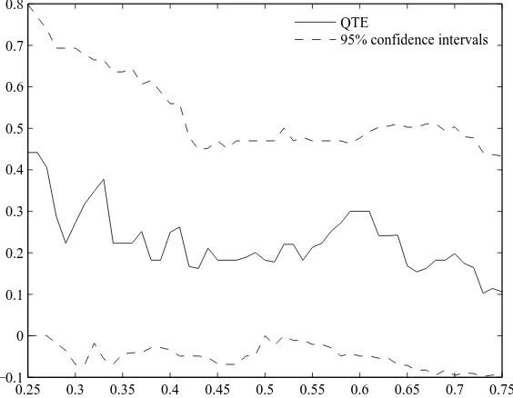
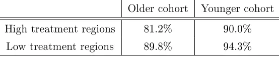
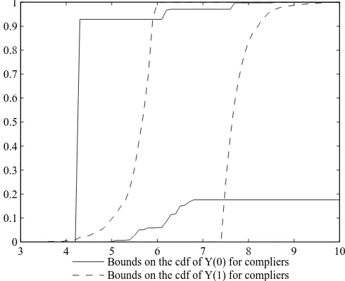
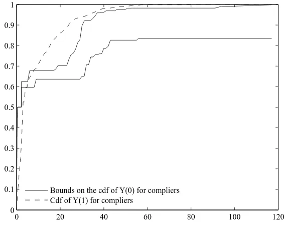
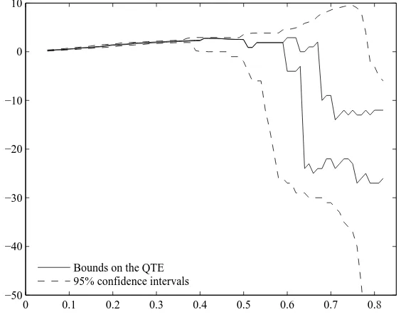
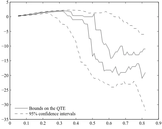
Finally, we apply our results to two dierent data sets. We rst revisit Field (2007), who studies the eect of granting property titles to urban squatters on their labor supply. As the treatment rate is stable in the comparison group used by the author, we are in the point iden-tied case. Our IV-CIC model allows us to study distributional eects of the treatment which were not studied by the author. We show that property rights have a stronger relative eect on households with a low initial labor supply. A possible explanation is that among squat-ters, only one household member has to stay home to look after the household's residence, irrespective of the household size. The eect of the program would then be large for small households with low initial labor supply, and smaller otherwise. Knowing this pattern of het-erogeneity might have substantial consequences on social choice. A utilitarian social planner will indeed be more prone to implementing a titling program with heterogeneous than with constant relative eects, provided utility of agents is concave in individual consumption. We then revisit results in Duo (2001) on returns to education. As the treatment rate changes in the comparison group used by the author, we are in the partially identied case. Our bounds are wide and uninformative, because the treatment rate increased substantially in the control group. Our IV-CIC model does not allow us to draw informative conclusions on returns to education from this natural experiment.
treatment eects, as we show in a third application developed in Appendix C. When exposition to treatment substantially changes in the control group as well, using our IV-CIC model will result in wide and uninformative bounds. In such instances, point identication can still be achieved using IV-DID, but at the price of imposing more stringent conditions.
Besides Athey & Imbens (2006), our paper is related to D'Haultfoeuille et al. (2013), who study the possibly nonlinear eects of a continuous treatment using repeated cross sections. They also rely on a control group to identify the eect of time, but in their case the choice of this group is driven by the data. Our paper is also connected to several recent papers analyzing dierence-in-dierences models. de Chaisemartin (2013) studies the identifying assumptions underlying IV-DID regressions. Several recent papers have also considered dierent routes from the one taken in Athey & Imbens (2006) to weaken the common trend condition in sharp DID. Blundell et al. (2004) and Abadie (2005) consider a conditional version of this assumption, and adjust for covariates using propensity score methods. Donald & Lang (2007) and Manski & Pepper (2012) allow for some variations in the way time aects the control and treatment groups, provided these variations satisfy some restrictions. Bonhomme & Sauder (2011) consider a linear model allowing for heterogeneous eects of time, and show how it can be identied using an instrument.
The remainder of the paper is organized as follows. Section 2 presents our model. Section 3 is devoted to identication. Section 4 presents some extensions. Section 5 deals with inference. In section 6 we apply our results to the two aforementioned data sets. Section 7 concludes. The appendix gathers all the proofs, some technical lemmas and a third application on the eect of a pharmacotherapy on smoking cessation.
2 The instrumental variable Changes-in-Changes model
LetT ∈ {0; 1} denote time and Gdenote the dummy of the treatment group (so that G= 0
for the control group). The treatmentDis supposed to be binary. Hereafter, for any random variablesR and S,R∼S means thatR andS have the same probability distribution. S(R)
andS(R|S) denote respectively the support ofR and the support of R conditional on S. As Athey & Imbens (2006), we introduce for any random variable R the corresponding random variablesRgt such that
Rgt∼R|G=g, T =t.
LetFRandFR|S denote the cumulative distribution function (cdf) ofRand its cdf conditional
onS. For any eventA,FR|Ais the cdf ofRconditional onA. With a slight abuse of notation,
real line, we denote byF−1 its generalized inverse:
F−1(q) = inf{x∈R/F(x)≥q}.
In particular, FX−1 is the quantile function of X. We adopt the convention that FX−1(q) = infS(X) for q <0, and FX−1(q) = supS(X)for q >1.
In our IV-CIC model, D6=G×T in general. Some units may be treated in the control group or at period 0, and all units are not necessarily treated in the treatment group at period 1.
This will arise when repeated cross sections are available, and the treatment is not tied to a strict rule. In such instances, it is not possible to know whether units at the second period were treated in the rst period, and we cannot dene a control group that was completely untreated in the rst period. When panel data are available, it may not be desirable to dene the treatment group as units going from non treatment to treatment, and the control group as units untreated at both periods. With this denition of groups, the assumptions underlying both the changes-in-changes model and the dierence-in-dierences model will be violated if individuals become treated because of an Ashenfelter's dip. Dening the control and treatment groups in an exogenous way usually makes the identifying assumption more credible. We let λd =P(D01 =d)/P(D00 =d) be the ratio of the shares of people receiving treatment d in period 1 and period 0 in the control group. For instance, λ0 > 1 when the share of untreated observations increases in the control group between period 0 and 1. λ0 >1 implies that λ1 <1 and conversely. µd=P(D11 =d)/P(D10=d) is the equivalent of λd for
the treatment group.
We assume that at period 1, individuals from the treatment group receive extra incentives to
get treated. We model this by introducing the binary instrumentZ =T×G. In Duo (2001), Z is an intensive school construction program which was implemented in treatment districts in period 1 and not in control ones, giving greater incentives to go to school to children living in those districts. The two corresponding potential treatments, D(1) and D(0), stand for
the treatment an individual would choose to receive with and without this supplementary incentive. The observed treatment is D = ZD(1) + (1−Z)D(0). Y(1) and Y(0) are the
potential outcomes of an individual with and without treatment. Implicit in this notation is the exclusion restriction that the instrument does not aect the outcome directly. The observed outcome is Y =DY(1) + (1−D)Y(0). As in Athey & Imbens (2006), we consider
the following model for the potential outcomes:
Y(d) =hd(Ud, T), d∈ {0; 1}. (1)
Assumption 1 (Monotonicity)
hd(u, t) is strictly increasing in u for all (d, t)∈ {0,1}2.
Assumption 2 (Latent index model for potential treatments)
D(z) = 1{V ≥vz(T)} with v0(t)> v1(t) for t∈ {0; 1}.
Assumption 3 (Time invariance within groups)
For d∈ {0,1}, (Ud, V)⊥⊥T|G.
Remarks on these assumptions are in order. Under Assumptions 1 and 2,V can be interpreted as a propensity for treatment. Similarly, if potential outcomes were schooling performances or wages, Ud could be interpreted as an ability index, and we stick to this interpretation
hereafter. Our latent index model is the same as in Vytlacil (2002), except that the threshold can depend on time, to allow for the treatment rate to evolve over time. As shown by Vytlacil (2002), such a latent index model is equivalent to the no deers condition in Imbens & Angrist (1994). Note that our results would not change ifUdandV were indexed by time, except that
we would have to rewrite Assumption 3 as follows: ford∈ {0,1}, Ud0, V0|G∼ Ud1, V1|G. This means we could allow individual ability and taste for treatment to change over time, provided their distribution remains the same in each group. Assumption 2 might seem to imply that time can aect individual treatment choice in only one direction. The previous discussion shows that this is actually not necessary for our results to hold. Time might induce some observations to go from non-treatment to treatment, while having the opposite eect on other observations. In what follows, we do not index Ud and V by time to alleviate the
notational burden, but it is worth bearing in mind that this is just an expositional choice, not a substantive restriction.
Assumption 3 requires that the joint distribution of ability and propensity for treatment re-mains stable in each group over time. It impliesUd⊥⊥T|GandV ⊥⊥T|G, which correspond
to the time invariance assumption in Athey & Imbens (2006). As a result, Assumptions 1-3 im-pose a standard CIC model both onY andD. But Assumption 3 also impliesUd⊥⊥T|G, V,
which means that in each group, the distribution of ability among people with a given taste for treatment should not change over time. This is the key supplementary ingredient with respect to the standard CIC model that we are going to use for identication.
thatY(d) =Ud+ηdT+γUdT, and that the standard CIC assumption is veried:
(U0, U1)⊥⊥T|G. (2)
This model allows for dierent trends in potential outcomes across ability levels and therefore across groups, because it does not impose that the distribution of U0 and U1 be the same in the two groups. It also allows for dierential trends for Y(0) and Y(1) through η0 and
η1. Combining this with the Roy model implies that selection into treatment can change over time. Finally, it satises Assumption 1 providedγ >−1. One can then rewrite
D(z) =1
U1−U0 ≥
c(z)−(η1−η0)T
1 +γT
.
Assumption 2 is satised with V = U1 −U0 and vz(T) = [c(z)−(η1 −η0)T]/(1 + γT). Therefore,(U0, U1)⊥⊥T|Gimplies that Assumption 3 is satised, becauseV is a deterministic function of U0 and U1. On the contrary, with γd instead of γ in the potential outcomes
equation, Assumption 3 cannot hold, becauseV = U1−U0+T(γ1U1−γ0U0). Assumption 3 is compatible with a Roy model in which time can have heterogeneous eects on outcomes across ability levels, and an homogeneous eect on propensity for treatment. But it is not compatible with a Roy model in which this second eect is heterogeneous across ability levels. Finally, it is worth mentioning that the IV-DID model is incompatible with the Roy selection model and outcome equations outlined above. As shown in de Chaisemartin (2013), in a model allowing for heterogeneous treatment eects, the IV-DID method relies on common trend assumptions both on potential outcomes and treatments. Common trend on potential treatments is necessary to ensure that the denominator of the Wald-DID ratio captures the size of the population induced to switch from non treatment to treatment between period 0 and 1 because of the instrument, not because of the eect of time alone. In the Roy model above, the common trend on potential outcomes implies that γ = 0. But even in this case,
the common trend on potential treatments does not hold in general. To see this, note that under (2), this condition is equivalent to
P(U1−U0 ≥c(z)−(η1−η0)|G= 1)−P(U1−U0 ≥c(z)|G= 1)
= P(U1−U0 ≥c(z)−(η1−η0)|G= 0)−P(U1−U0 ≥c(z)|G= 0).
This is unlikely to be true, unless we are ready to assume thatU1−U0 ⊥⊥G. But this would amount to assuming that groups are as good as randomly assigned, in which case we do not need to resort to a longitudinal analysis to capture treatment eects. We could merely use a standard cross-sectional IV using group as an instrument for treatment in period 1.
those in Athey & Imbens (2006) when P(D11 = 1) = 1 and P(D10 = 1) = P(D01 = 1) =
P(D00= 1) = 0, namely when their sharp setting holds.
Finally, we impose the two following restrictions, which are directly testable in the data.
Assumption 4 (Data restrictions)
1. S(Ygt|D=d) =S(Y) = [y, y]with (y, y)∈R2, for (g, t, d)∈ {0; 1}3.
2. FYgt|D=d is strictly increasing and continuous on S(Y), for (g, t, d)∈ {0; 1}3.
Assumption 5 (Rank conditions)
1. P(D11= 1)−P(D10= 1)>0.
2. IfP(D00= 0)>0,FY10|D=0◦F −1
Y00|D=0(λ0)> µ0andFY10|D=0◦F −1
Y00|D=0(1−λ0)<1−µ0.
The rst condition of Assumption 4 is a common support condition. Athey & Imbens (2006) take a similar assumption and show how to derive partial identication results when it is not veried. Point 2 is satised if the distribution ofY is continuous with positive density in each of the eight groups×period ×treatment status cells.
Assumption 5 corresponds to a rank condition in a standard IV model. The IV-CIC identica-tion strategy requires that treatment rate changes in at least one group. If it diminishes in the two groups over time we can just switch labels and consider1−D as the treatment variable. Therefore, the rst condition is without loss of generality: it does not impose anything except that treatment rate changes in at least one group.
To better understand the second condition of Assumption 5, let us draw a parallel with the IV-DID model. The rank condition in an IV-DID regression is
P(D11= 1)−P(D10= 1)−(P(D01= 1)−P(D00= 1))6= 0,
large eect on the share of people receiving treatment. IfFY10|D=0◦FY−001|D=0 is the identity
function, this condition will be veried if and only ifλ0> µ0. In practice,FY10|D=0◦F −1
Y00|D=0
might not be the identity function, but this still shows that the larger the dierence between λ0 andµ0, the more likely this condition holds.
Finally, it should be emphasized that as the rst condition, the second condition of Assumption 5 is testable from the data, so it can be assessed beforehand by researchers willing to use our IV-CIC model. When this test is rejected, our model cannot be used as it will only yield trivial bounds for treatment eects, as we will explain below.
Before getting to the identication results, it is useful to dene ve subpopulations of interest. Assumption 3 implies that P(D10 = 1) = P(V ≥ v0(0)|G = 1), and similarly P(D11 =
1) = P(V ≥ v1(1)|G = 1). Therefore, under Assumption 5, v0(0) > v1(1). Similarly, if the treatment rate increases (resp. decreases) in the control group, v0(0) > v0(1) (resp.
v0(0)< v0(1)). Finally, assumption Assumption 2 implies v1(1) ≤v0(1). Let always takers be such thatV ≥v0(0), and let never takers be such thatV < v1(1). Always takers are units who get treated in period 0 even without receiving any incentive for treatment. Never takers are units who do not get treated in period 1 even after receiving an incentive for treatment. Let T C = V ∈ [min(v0(0), v0(1)),max(v0(0), v0(1))). T C stands for time compliers, and represents observations whose treatment status switches between the two periods because of the eect of time. Similarly, letIC =V ∈[v1(1), v0(1)).2 IC stands for instrument compliers. This population corresponds to compliers as per the denition of Imbens & Angrist (1994), that is to say observations that become treated through the eect of Z only. However, in our IV-CIC model, we cannot learn anything on this population. Instead, our identication results focus on observations that satisfy V ∈ [v1(1), v0(0)). This corresponds to untreated observations at period 0 who become treated at period 1, through both the eect of Z and time. We refer to those observations as compliers to simplify the exposition, and we let hereafterC denote the eventV ∈[v1(1), v0(0)). If the treatment rate increases in the control group (i.e. if v0(1) < v0(0)), we merely have C = IC ∪T C, while if it decreases we have
C=IC\T C.
Our parameters of interest are the cdf of Y(1) and Y(0) among compliers, as well as the
Local Average Treatment Eet (LATE) and Quantile Treatment Eects (QTE) within this population, which are respectively dened by
∆ = E(Y11(1)−Y11(0)|C),
τq = FY−111(1)|C(q)−FY−111(0)|C(q), q∈(0,1).
2IC is dened to be empty whenv
3 Identication
3.1 Point identication results
We rst show that when the treatment rate does not change between the two periods, the cdf ofY(1)andY(0)among compliers are identied. Consequently, the LATE and QTE are also
point identied. Let Qd(y) = FY−011|D=d◦FY00|D=d(y) be the the quantile-quantile transform
of Y from period 0 to 1 in the control group conditional on D = d. This transform maps y at rank q in period 0 into the corresponding y0 at rank q as well in period 1. Also, let
QD =DQ1+ (1−D)Q0. Finally, let Hd(q) =FY10|D=d◦F −1
Y00|D=d(q) be the inverse
quantile-quantile transform of Y from the control to the treatment group in period 0 conditional on D=d. This transform maps rankqin the control group into the corresponding rankq0 in the treatment group with the same value ofy.
Theorem 3.1 If Assumptions 1-5 hold and for d ∈ {0,1} P(D00 = d) = P(D01 =d) > 0,
FY11(d)|C(y) is identied by
FY11(d)|C(y) =
P(D10=d)FQd(Y10)|D=d(y)−P(D11=d)FY11|D=d(y)
P(D10=d)−P(D11=d)
= P(D10=d)Hd◦FY01|D=d(y)−P(D11=d)FY11|D=d(y)
P(D10=d)−P(D11=d)
.
This implies that ∆and τq are also identied. Moreover,
∆ = E(Y11)−E(QD(Y10))
E(D11)−E(D10)
.
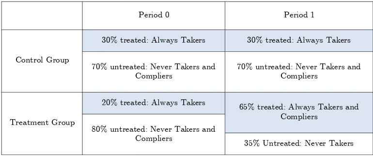
This theorem combines ideas from Imbens & Rubin (1997) and Athey & Imbens (2006). We seek to recover the distribution of Y(1)andY(0)among compliers in the treatment ×period 1 cell. When the treatment rate does not change in the control group, v0(0) = v0(1). As a result, there are no time compliers, and compliers are merely instrument compliers. To recover the distribution of Y(1)among them, we start from the distribution of Y among all treated observations of this cell. As shown in Table 1, those include both compliers and always takers. Consequently, we must withdraw from this distribution the cdf ofY(1)among always
takers, exactly as in Imbens & Rubin (1997). But this last distribution is not observed. To reconstruct it, we adapt the ideas in Athey & Imbens (2006). As is shown in Table 1, all treated observations in the control group or in period 0 are always takers; the distribution of Y(1)among always takers is identied within those three cells. Since Assumption 3 implies
U1 ⊥⊥T|G, V ≥v0(0),
and 1 among always takers of the treatment group. This implies that the quantile-quantile transform among always takers is the same in the treatment and control groups. As a result, we can identify the distribution ofY(1)among treatment ×period 1 always takers, applying the quantile-quantile transform from period 0 to 1 among treated observations in the control group to the distribution of Y(1) among always takers in the treatment group in period 0.
Identication of the distribution ofY(0)among compliers in the treatment×period 1cell is
obtained through similar steps.
Treatment Group
20% treated: Always Takers
65% treated: Always Takers and
Compliers 80% untreated: Never Takers and
Compliers
35% Untreated: Never Takers Period 0 Period 1
Control Group
30% treated: Always Takers 30% treated: Always Takers
70% untreated: Never Takers and Compliers
[image:15.612.108.493.243.404.2]70% untreated: Never Takers and Compliers
Table 1: Populations of interest whenP(D00= 0) =P(D01= 0).
Another way to understand the transform we use to reconstruct the cdf ofY(1)among always
takers is to regard it as a double matching. Consider an always taker in the treatment × period 0 cell. She is rst matched to an always taker in the control × period 0 cell with samey. Those two always takers are observed at the same period of time and have the same treatment status. Therefore, under assumption Assumption 1 they must have the same u1. Second, the control ×period 0always taker is matched to its rank counterpart among always
takers of the control × period 1 cell (this is merely the quantile-quantile transform). We denote y∗ the outcome of this last observation. Because U1 ⊥⊥ T|G, V ≥ v0(0), those two observations must also have the same u1. Consequently, y∗ =h1(u1,1), which means that y∗ is the outcome that the treatment×period 0 cell always taker would have obtained in period 1. Therefore, to recover the whole distribution of Y(1)in period 1 among test group always
Note that our LATE estimand is similar to the LATE estimand in Imbens & Angrist (1994), the standard Wald ratio. Once noted that conditional onG= 1,Z =T, we have
∆ = E(Y|G= 1, Z = 1)−E(QD(Y)|G= 1, Z = 0)
E(D|G= 1, Z = 1)−E(D|G= 1, Z = 0) .
The Wald ratio has the same expression, except that here Y is replaced by QD(Y) in the
second term of the numerator. The standard Wald parameter does not identify a causal eect here because conditional on G= 1, Z (i.e. T) is not independent of Y(d): the distributions
of potential outcomes might evolve with time. To take into account the eect of time on the distribution of potential outcomes, we apply the quantile-quantile transform observed between period 0 and 1 in the control group to the distribution ofY in period 0 in the treatment group. Assumptions 1 and 3 ensure that quantile-quantile transforms are the same in the two groups. Likewise, the formulae of the cdf ofY(1)andY(0)among compliers are very similar to those
obtained in Imbens & Rubin (1997). For instance, the cdf of Y(1) rewrites as
P(D= 1|G= 1, Z= 1)FY|D=1,G=1,Z=1(y)−P(D= 1|G= 1, Z= 0)FQ1(Y)|D=1,G=1,Z=0(y)
P(D= 1|G= 1, Z= 1)−P(D= 1|G= 1, Z= 0) .
The cdf of Y(1) in the Imbens and Angrist IV model has the same expression except that
Q1(Y)is replaced byY in the second term of the numerator. Here again, this is to account for the fact that conditional onG= 1, the instrumentT is not independent of potential outcomes. Under Assumptions 1-5, the LATE and QTE for compliers are point identied when 0 < P(D00 = 0) =P(D01 = 0)<1, but not in the extreme cases where P(D00= 0) = P(D01=
0) ∈ {0,1}. For instance, when P(D00 = 1) = P(D01 = 1) = 1, FY11(1)|C is identied by
Theorem 3.1, butFY11(0)|C is not. Such situations are likely to arise in practice, for instance
when a policy is extended to a previously ineligible group, or when a program or a technology previously available in some geographic areas is extended to others (see Subsection 6.1 below). We therefore consider a mild strengthening of our assumptions under which bothFY11(0)|C and
FY11(1)|C are point identied in those instances.
Assumption 6 (Common eect of time on both potential outcomes) h0(u, t) = h1(u, t) =
h(u, t) for every (u, t)∈ S(U)× {0,1}.
Assumption 6 requires that the eect of time be the same on both potential outcomes. It implies that two observations with the same outcome in period 0 will also have the same outcome in period 1 if they do not switch treatment between the two periods, even if they do not share the same treatment at period 0. Under this assumption, ifP(D00= 1) =P(D01=
1) = 1, changes in the distribution of Y in the control group over time allow us to identify the eect of time both on Y(0) and Y(1), hence allowing us to recover both FY11(0)|C and
Theorem 3.2 If Assumptions 1-6 hold and P(D00 = d) = P(D01 = d) = 0 for some d ∈ {0,1},FY11(d)|C(y) andFY11(1−d)|C(y) are identied by
FY11(d)|C(y) =
P(D10=d)FQ1−d(Y)10|D=d(y)−P(D11=d)FY11|D=d(y)
P(D10=d)−P(D11=d)
FY11(1−d)|C(y) =
P(D10= 1−d)FQ1−d(Y)10|D=1−d(y)−P(D11= 1−d)FY11|D=1−d(y)
P(D10= 1−d)−P(D11= 1−d)
.
This implies that ∆and τq are also identied. Moreover,
∆ = E(Y11)−E(Q1−d(Y10))
E(D11)−E(D10)
.
A last situation worth noting is when the treatment rate is equal to 0 at both dates in the
control group, and is also equal to 0 in the rst period in the treatment group. This is a
special case of Theorem 3.2, but in such instances we can actually identify the model under fewer assumptions. To see this, note that in such situations,
FY11(1)|C =FY11|D=1 (3)
because there are no always takers in the treatment group. Therefore, we only need to recover FY11(0)|C. But since the distribution of Y11(0) among never takers is identied by FY11|D=0,
under Assumption 2 we only need to recoverFY11(0). This can be achieved under the standard changes-in-changes assumptions, as the control group remains fully untreated at both dates.
3.2 Partial identication
When P(D00 = d) =P(D01 =d), FY11(d)|C is identied under Assumptions 1-5 or
Assump-tions 1-6. We shall show below that if this condition is not veried, the funcAssump-tionsFY11(d)|C are
partially identied. For that purpose, we must distinguish between two cases.
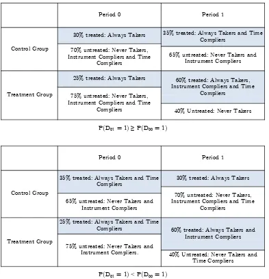
The rst one is when P(D00 = d) > 0. In such instances, the rst of the two matchings described in the previous section works as before. But the second one collapses, since we no longer have v0(1) = v0(0). Among treated observations in the control × period 0 cell,
U1 is distributed conditional on G = 0, V ≥ v0(0), while it is distributed conditional on
compliers can be written as functions of observed distributions and ofFY01(d)|T C, in a formula
where FY01(d)|T C enters with a weight identied from the data.
35% treated: Always Takers and Time Compliers
65% untreated: Never Takers and Instrument Compliers
70% untreated: Never Takers, Instrument Compliers and Time
Compliers
25% treated: Always Takers and Time
Compliers 60% treated: Always Takers and Instrument Compliers 75% untreated: Never Takers and
Instrument Compliers. 40% Untreated: Never Takers and Time Compliers
30% treated: Always Takers
P(D01 = 1) < P(D00 = 1)
Period 1
Control Group
Treatment Group
Period 0
P(D01 = 1) ≥ P(D00 = 1)
Treatment Group Control Group
35% treated: Always Takers and Time Compliers
Period 0 Period 1 30% treated: Always Takers
70% untreated: Never Takers, Instrument Compliers and Time
Compliers
65% untreated: Never Takers and Instrument Compliers
25% treated: Always Takers
75% untreated: Never Takers, Instrument Compliers and Time
Compliers
60% treated: Always Takers, Instrument Compliers and Time
Compliers
[image:18.612.107.500.156.564.2]40% Untreated: Never Takers
Table 2: Populations of interest.
The second case we have to consider is whenP(D00 =d) = 0. In this case, the rst step of the aforementioned double matching collapses for the distribution of Y(d). For instance, if
P(D00 = 1) = 0, there are no treated observations in the control group in period 0 to which treated observations in the treatment group in period 0 can be matched. Still, the cdf of Y among treated observations in the treatment ×period 1 cell writes as a weighted average of the cdf of Y(d) among compliers and always or never takers. We can use this fact to bound
The following lemma summarizes these results. To derive bounds onFY11(d)|C and then on the
LATE and QTE, we rst relate these cdf to observed distributions and one unidentied cdf.
Lemma 3.1 If Assumptions 1-5 hold, then:
- If P(D00=d)>0,
FY11(d)|C(y) =
P(D10=d)Hd◦(λdFY01|D=d(y) + (1−λd)FY01(d)|T C(y))−P(D11=d)FY11|D=d(y)
P(D10=d)−P(D11=d)
.
- If P(D00=d) = 0,
FY11(d)|C =
P(D10=d)FY11(d)|(2d−1)V >(2d−1)v0(0)−P(D11=d)FY11|D=d
P(D10=d)−P(D11=d)
.
From this lemma, it appears that whenP(D00=d)>0, we merely need to boundFY01(d)|T C to
derive bounds onFY11(d)|C. In order to do so, we must take into account the fact thatFY01(d)|T C
is related to two other cdf. To alleviate the notational burden, let Td=FY01(d)|T C,Cd(Td) =
FY11(d)|C, G0(T0) = FY01(0)|V <v0(0) and G1(T1) = FY01(1)|V≥v0(0). With those notations, we
have
Gd(Td) = λdFY01|D=d+ (1−λd)Td
Cd(Td) =
P(D10=d)Hd◦Gd(Td)−P(D11=d)FY11|D=d
P(D10=d)−P(D11=d)
.
The fact thatTd,Gd(Td) andCd(Td) should all be included between 0 and 1 imposes several
restrictions on Td, from which we derive our bounds. Let M0(x) = max(0, x), m1(x) =
min(1, x) and dene
Td = M0 m1
λdFY01|D=d−H −1
d (µdFY11|D=d)
λd−1
!!
,
Td = M0 m1
λdFY01|D=d−H −1
d (µdFY11|D=d+ (1−µd))
λd−1
!!
.
When P(D00 = d) > 0, we can bound FY11(d)|C by Cd(Td) and Cd(Td). These bounds can
however be improved by remarking that FY11(d)|C is increasing. Therefore, we dene our
bounds as:
Bd(y) = supy0≤yCd(Td) (y0),
Bd(y) = infy0≥yCd Td(y0).
(4)
When P(D00 = d) = 0, the bounds on FY11(d)|C are much simpler. We simply bound
FY11(1)|(2d−1)V≥(2d−1)v0(0) by 0 and 1, which yields
Bd(y) =M0
P(D
10=d)−P(D11=d)FY11|D=d
P(D10=d)−P(D11=d)
, Bd(y) =m1
−P(D
11=d)FY11|D=d
P(D10=d)−P(D11=d)
Ford= 0, the bounds are actually trivial since B0(y) = 0 and B1(y) = 1.
Another important case where the bounds take a simple form is whenP(D10 = 1) = 0. In this case, one can check that
B1=B1=FY11|D=1.
This is because in such situations, FY11(1)|C =FY11|D=1 as shown in Equation (3).
Theorem 3.3 proves that Bd and Bd are indeed bounds for FY11(d)|C. We also consider the
issue of whether these bounds are sharp or not. Hereafter, we say that Bd is sharp (and similarly forBd) if there exists a sequence of cdf(Gk)k∈N such that supposingFY11(d)|C =Gk
is compatible with both the data and the model, and for ally,limk→∞Gk(y) =Bd(y). We
establish thatBdand Bd are sharp under Assumption 7 below. Note that this assumption is
testable from the data.
Assumption 7 (Increasing bounds)
For(d, g, t)∈ {0,1}3,F
Ygt|D=dis continuously dierentiable, with positive derivative on
◦
S(Y).
Moreover, either (i) P(D00 =d) = 0 or (ii)Td, Gd(Td) and Cd(Td) (resp. Td, Gd(Td) and
Cd(Td)) are increasing.
Theorem 3.3 If Assumptions 1-5 hold, we have
Bd(y)≤FY11(d)|C(y)≤Bd(y).
Moreover, if Assumption 7 holds, Bd(y) and Bd(y) are sharp.
The intuition underlying the sharpness result goes as follows. LetTdbe the set of all functions Td increasing and included between 0 and 1 such thatGd(Td) andCd(Td) are also increasing
and included between 0 and 1. T0 is the set of all cdf FY01(0)|T C such thatFY01(0)|V <v0(0) and
FY11(0)|C are cdf. This suggests that Td is the set of all candidates for FY01(d)|T C that can be
rationalized by the data and the model. Now, assume that there existsT0− andT0+inT0 such thatT0−≤T0≤T0+ for every T0∈ T0. Whenλ0 >1,G0(.) is decreasing inT0, which implies thatC0(.)is also decreasing inT0. Therefore, in such instances the sharp lower bound ofC0(.) is equal toC0(T0+), while the sharp upper bound is equal toC0(T0−). Moreover, whenλ0 >1, it appears after some algebra thatT0,G0(T0) and C0(T0) are all included between 0 and 1 if and only if T0 ≤T0 ≤ T0. Therefore, if T0, G0(T0) and C0(T0) are increasing, T0 is in T0 and T0+=T0. This implies that B0 =C0(T0) is sharp under Assumption 7. Whenλ0<1, a similar reasoning also shows thatB0 =C0(T0) is sharp under Assumption 7.
reason for this asymmetry is that whenλ0 <1, time compliers belong to the group of treated observations in the control ×period 1 cell (cf. Table 2). Therefore, theirY(0)is not observed
in period 1, and the data does not impose any restriction on FY01(0)|T C: it could be equal
to 0 or to 1, hence the defective bounds. On the contrary, when λ0 > 1, time compliers belong to the group of untreated observations in the control×period 1 cell. Moreover, under Assumption 3, we know that they account for 100(1−1/λ0)% of this group. Consequently, the data imposes some restrictions on FY01(0)|T C. For instance, we must have
FY01|D=0,Y≥α≤FY01(0)|T C ≤FY01|D=0,Y≤β,
where α = FY−1
01|D=0(1/λ0) and β = F −1
Y01|D=0(1−1/λ0). The cdf of time compliers cannot
be below the one of the 100(1−1/λ0)% of observations with highest Y of this group, and cannot be above the one of the 100(1−1/λ0)% of observations with lowest Y of this group.
B0 andB0 are trimming bounds in the spirit of Horowitz & Manski (1995) whenλ0>1, but not whenλ0 <1, which is the reason why they are defective then.
Another interesting asymmetry is thatB1 andB1 are always proper cdf, while we could have expected them to be defective when λ0 > 1, because then time compliers are untreated in period 1, so their Y(1)is unobserved. This second asymmetry stems from the fact that when
λ0 >1, time compliers do not belong to our population of compliers (C =IC \T C), while when λ0 <1, time compliers are included within our population of interest (C =IC ∪T C). Setting FY01(1)|T C(y) = 0 does not imply that limy→+∞FY11(1)|C(y) < 1 when T C ∩C is
empty, while settingFY01(0)|T C(y) = 0 yields limy→+∞FY11(0)|C(y)<1 whenT C ⊂C.
Finally, one can check thatlimy→yB0(y) =M0
P(D
10=0)H0(λ0)−P(D11=0)
P(D10=0)−P(D11=0)
, whilelimy→yB0(y) =
m1
P(D
10=0)H0(1−λ0)
P(D10=0)−P(D11=0)
. Under Assumption 5, the rst limit is strictly greater than 0 and
the second one is strictly lower than 1, which implies that our two bounds are non trivial.
If Assumption 5 is violated, at least one of our two bounds is trivial, which implies that for every quantile treatment eect one of our two bounds will either be+∞or −∞.
A consequence of Theorem 3.3 is that QTE and LATE are partially identied whenP(D00=
0)6= P(D01 = 0) or P(D00 = 0) ∈ {0,1}. The bounds are given in the following corollary. To ensure that the bounds on the LATE are well dened, we impose the following technical condition.
Assumption 8 (Existence of moments)
R
|y|dB1(y)<+∞ and
R
|y|dB1(y)<+∞.3
3R
|y|dB1(y)is the integral of the absolute value function with respect to the probability measureνdened
on[y, y]and generated byB1. The same holds for
R
|y|dB1(y),R
|y|dB0(y)and
R
|y|dB0(y). Because we may
Corollary 3.4 If Assumptions 1-5 and 8 hold andP(D00= 0)6=P(D01= 0) ,∆and τq are
partially identied, with
Z
ydB1(y)−
Z
ydB0(y)≤∆≤
Z
ydB1(y)−
Z
ydB0(y),
max(B−11(q), y)−min(B−01(q), y)≤τq ≤min(B1−1(q), y)−max(B
−1 0 (q), y).
Moreover, suppose that Assumption 7 holds. Then
- If λ0 >1 or E(|Y11(0)| |C)<+∞, the bounds on ∆are sharp.
- If λ0 > 1 or for d ∈ {0,1}, Bd(y) = q and Bd(y) = q admit a unique solution, the
bounds on τq are sharp.
Whenλ0 <1 and S(Y) is unbounded, the bounds on∆are innite, and some bounds on τq
are also innite. On the contrary, whenλ0 >1 the bounds onτq are always nite, for every
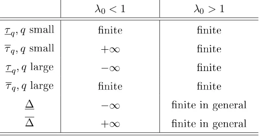
[image:22.612.175.431.438.573.2]q ∈ (0,1). The bounds on the LATE will also be nite in this case, as soon as B0 and B0 admit an expectation. Table 3 summarizes the situation.
Table 3: Finiteness of the bounds wheny=−∞, y= +∞.
λ0 <1 λ0>1
τq, q small nite nite
τq, q small +∞ nite
τq, qlarge −∞ nite
τq, qlarge nite nite
∆ −∞ nite in general
∆ +∞ nite in general
qsmall means0< q < qfor a well chosenq. Similarly, q large meansq < q <1for a well chosenq.
4 Extensions
4.1 Identication of a conditional IV-CIC model
assumption and to outline two more strategies to recover point identication whenP(D00=
d)6=P(D01=d).
Letλd,x =P(D01 =d|X =x)/P(D00 =d|X =x) and µd,x =P(D11 =d|X =x)/P(D10 =
d|X=x). Assume that
Y(d) =hd(Ud, T, X), d∈ {0; 1},
and substitute the following assumptions to Assumptions 1-5:
Assumption 9 (Monotonicity 2)
hd(u, t, x) is strictly increasing inu for all (d, t, x)∈ {0,1}2× S(X).
Assumption 10 (Latent index model for potential treatments 2)
D(z) = 1{V ≥vz(T, X)} with v0(t, x)> v1(t, x) for (t, x)∈ {0; 1} × S(X).
Assumption 11 (Conditional time invariance) For d∈ {0,1}, (Ud, V)⊥⊥T|G, X.
Assumption 12 (Data restrictions 2)
1. S(Xgt|D=d) =S(X) = [x, x] with (x, x)∈R2.
2. S(Ygt|D=d, X =x) =S(Y) = [y, y] with (y, y)∈R2, for (g, t, d, x)∈ {0; 1}3× S(X).
3. FYgt|D=d,X=x is strictly increasing and continuous on S(Y), for (g, t, d, x) ∈ {0; 1}3×
S(X).
Assumption 13 (Changes in the treatment rates 2) For every x∈ S(X),
1. P(D11= 1|X=x)−P(D10= 1|X =x)>0.
2. IfP(D00= 0|X=x)>0, FY10|D=0,X=x◦F −1
Y00|D=0,X=x(λ0,x)> µ0,x andFY10|D=0,X=x◦
FY−1
00|D=0,X=x(1−λ0,x)<1−µ0,x.
Incorporating covariates allows us to weaken the main identifying assumption of our model. When the distribution of someX evolves over time in the control or in the treatment group, Assumption 11 might be more credible than Assumption 3: if the distribution of X is not stable over time andX is correlated to(Ud, V), then the distribution of(Ud, V)might not be
stable either.
Lemma 4.1 Suppose that Assumptions 9-13 hold. Then,
fX11|C(x) =
[P(D11= 1|X =x)−P(D10= 1|X =x)]fX11(x)
E[P(D11= 1|X)−P(D10= 1|X)|G= 1, T = 1]
Then, the conditional IV-CIC assumptions imply that the IV-CIC assumptions are satised conditional on X, so one can prove conditional versions of Theorems 3.1 and 3.3. This im-plies that for every d ∈ {0,1}, FY11(d)|C,X=x(y) is point identied whenever 0 < P(D00 =
d|X = x) = P(D01 = d|X = x), while it is partially identied otherwise. One can then integrateFY11(d)|C,X=x(y) or its bounds over the distribution ofX11among compliers to point
or partially identifyFY11(d)|C(y). This idea is formalized in the following theorem, in the point
identied case. Hereafter, we letQd,x(y) =FY−011|D=d,X=x◦FY00|D=d,X=x(y).
Theorem 4.1 Suppose Assumptions 9-13 hold. If 0 < P(D00 = d|X) = P(D01 = d|X) almost surely, the conditional distribution of potential outcomes on compliers is identied by
FY11(d)|X=x,C(y) =
P(D10=d|X=x)FQd,x(Y10)|D=d,X=x(y)−P(D11=d|X =x)FY11|D=d,X=x(y)
P(D10=d|X=x)−P(D11=d|X =x)
.
The overall distribution of potential outcomes among compliers is also identied.
This theorem is useful when P(D00 = d) 6= P(D01 = d) but P(D00 = d|X) = P(D01 =
d|X) > 0 almost surely, meaning that in the control group, the evolution of the treatment
rate is entirely driven by a change in the distribution of X over time. Otherwise, we can of course obtain bounds, using a similar argument as in Theorem 3.3. The bounds are likely to be tighter than the unconditional ones if X drives most of the evolution of the treatment rate in the control group.
We also consider another assumption under which treatment eects are still point identied, even if the treatment rate evolves in some X cells of the control group.
Assumption 14 (Strong conditional time invariance)
Ud⊥⊥T|G= 0, D(0) =d, X
When P(D00 = 0|X = x) = P(D01 = 0|X = x), Assumption 11 implies that Assumption 14 holds in the X =x cell. But this is no longer true when P(D00 = 0|X =x)6= P(D01 =
0|X = x). Then, Assumption 14 requires that even though selection into treatment might
treatment. IfP(D00 = 0|X=x)< P(D01= 0|X =x), a sucient condition for that to hold in theX=x cell is
Ud⊥⊥V|G= 0, T =d, D(0) =d, X =x, d∈ {0,1}.
This is reminiscent of the ignorability condition in Rosenbaum & Rubin (1983), even though we believe it is weaker. Ignorability states that selection is exogenous after controlling forX. Here we posit that the propensity for the treatment is exogenous after controlling for bothX andD(0).
Theorem 4.2 Suppose Assumptions 9-13 and 14 hold. The conditional distributions of po-tential outcomes on compliers are identied by
FY11(d)|X=x,C(y) =
P(D10=d|X=x)FQd,x(Y)10|D=d,X=x(y)−P(D11=d|X =x)FY11|D=d,X=x(y)
P(D10=d|X =x)−P(D11=d|X=x)
ford∈ {0,1}. The overall distribution of potential outcomes among compliers is also identied.
4.2 Several periods and groups
Results of Section 3 can also be extended to settings with many groups. This will increase the chances that we can recover point identication, provide us with a test of our model, and at the very least tighten our bounds relative to the two groups case. If the treatment rate is stable in at least one group, which is likely to be the case with many groups, one can use it as a control group and point identify treatment eects in period 1 among compliers in every group in which the treatment rate changes between the two periods.4 If there are several
groups in which the treatment rate remains stable between the two periods, one can use either of those groups as a control for other groups. This provides us with a test of our IV-CIC model, as the quantile-quantile transforms of the outcome should be the same in all these control groups. Formally, FY−1
g0|D=d◦FYg1|D=d should not depend on g, for any g such that
P(Dg1= 0) =P(Dg0 = 0). If the treatment rate changes in every group, then for each group we can derive bounds for the cdf of Y(0) and Y(1) among compliers using any other group
satisfying Assumption 5 as a control group, and we can tighten the various bounds obtained by using intersection bounds (see Chernozhukov et al., 2013).
The previous results can also be extended to settings with many time periods, which will increase even more more the chances of recovering point identication. With more than two 4For groups in which the treatment rate diminishes over the two periods, one can just switch labels and
consider 1−D as the treatment variable. As explained before, the rst condition in Assumption 5 is just
a normalization. Doing this, we recover the opposite of the LATE and QTE, for a population of compliers dened dierently (the individuals who switch fromD= 1toD= 0either because of time or because of the
periods, if the treatment rate is stable in at least one group between periodt−kandtfor some k, one can use it as a control group and point identify treatment eects in period t among compliers in every group in which the treatment rate changes betweent−k andt. However, our time invariance assumption might be less credible when the number of time periods grows, since groups are more likely to evolve over a long time period.
4.3 Testability
We show now that our IV-CIC model is testable. We focus here on the unconditional model described in Section 2, but similar implications could be obtained for the conditional models considered above. For everyy≤y0 inS(Y)2, let
Id(y, y0) = [min(Td(y), Td(y)),max(Td(y
0
), Td(y0))],
with the convention thatId(y, y0) =∅ if
min(Td(y), Td(y))>max(Td(y
0
), Td(y0)).
Theorem 4.3 If Assumption 4 holds, we reject Assumptions 1-3 together if for some d ∈ {0; 1}, one of the two following statements holds:
1. For some y0 ≤y1 in S(Y)2, Id(y0, y1) =∅.
2. For some y0 < y1 in S(Y)2, Id(y0, y1)6=∅ but for every t0≤t1 in Id(y0, y1)2,
P(D10=d)Hd◦(λdFY01|D=d(y1) + (1−λd)t1)−P(D11=d)FY11|D=d(y1)
P(D10=d)−P(D11=d)
< P(D10=d)Hd◦(λdFY01|D=d(y0) + (1−λd)t0)−P(D11=d)FY11|D=d(y0)
P(D10=d)−P(D11=d)
.(5)
Theorem 4.3 provides a theoretical test of the model. When the treatment rate does not change in the control group, i.e. when λd = 1, the two testable implications of the IV-CIC
model reduce to having that
P(D10=d)Hd◦FY01|D=d(y)−P(D11=d)FY11|D=d(y)
P(D10=d)−P(D11=d)
is increasing. Therefore, in such instances, our test is similar to the one developed by Kitagawa (2013) for the instrumental variable model in Angrist et al. (1996) with binary treatment and instrument. In their model, the cdf of compliers can also be written as the dierence between two increasing functions, and thus may not be increasing (see Imbens & Rubin, 1997).
some d∈ {0,1}, i.e. when there is no function Td such thatGd(Td) and Cd(Td) are also cdf,
while such a function should exist under Assumptions 1-3 as shown in Lemma 3.1. We give two sucient conditions under whichTdis empty. To understand them, remark thatId(y, y0)2
includes the set of all possible values forTd(y) and Td(y0)such that Td(y),Td(y0),Gd(Td)(y),
Cd(Td)(y),Gd(Td)(y0), andCd(Td)(y0)are included between0and1. IfId(y0, y1) is empty for somey0 ≤y1,Td must be empty. If point 2 holds,Td is also empty because it is not possible
to dene Td(y0) and Td(y1) such that 0 ≤ Td(y0) ≤ Td(y1) ≤ 1, Gd(Td)(y0), Gd(Td)(y1),
Cd(Td)(y0)and Cd(Td)(y1) are included between 0 and 1 andCd(Td)(y0)≤Cd(Td)(y1).
The test presented in point 2 is much simpler to implement whenλ0 <1 than when λ0 >1. Whenλ0 <1,
P(D10=d)Hd◦(λdFY01|D=d(y) + (1−λd)t)−P(D11=d)FY11|D=d(y)
P(D10=d)−P(D11=d)
is increasing in t. Therefore, one necessary and sucient condition for inequality (5) to hold in this case is that there exists y0≤y1 inS(Y)2 such that for somed∈ {0,1},
P(D10=d)Hd◦(λdFY01|D=d(y1) + (1−λd) max(Td(y1), Td(y1)))−P(D11=d)FY11|D=d(y1)
P(D10=d)−P(D11=d)
< P(D10=d)Hd◦(λdFY01|D=d(y0) + (1−λd) min(Td(y0), Td(y0)))−P(D11=d)FY11|D=d(y0)
P(D10=d)−P(D11=d)
.
In contrast, when λ0 >1,
P(D10=d)Hd◦(λdFY01|D=d(y) + (1−λd)t)−P(D11=d)FY11|D=d(y)
P(D10=d)−P(D11=d)
is decreasing in t. Then, one necessary and sucient condition for inequality (5) to hold in this case is that there existsy0 < y1 inS(Y)2 such that for some d∈ {0,1} and for everytin
I(y0, y1),
P(D10=d)Hd◦(λdFY01|D=d(y1) + (1−λd)t)−P(D11=d)FY11|D=d(y1)
P(D10=d)−P(D11=d)
< P(D10=d)Hd◦(λdFY01|D=d(y0) + (1−λd)t)−P(D11=d)FY11|D=d(y0)
P(D10=d)−P(D11=d)
.
Whenλ0 <1, for every y0 < y1 the test will amount to assessing inequality (5) for only one value of(t0, t1). When λ0 >1, for everyy0 < y1 the test will amount to assessing Inequality (5) for an innity of(t0, t1), unlessI(y0, y1) reduces to a point.
5 Inference
Assumption 15 (Independent and identically distributed observations)
(Yi, Di, Gi, Ti)i=1,...,n are i.i.d.
Assumption 16 (Technical conditions for inference 1)
S(Y) is a bounded interval [y, y]. Moreover, for all (d, g, t) ∈ {0,1}3, F
dgt = FYgt|D=d and
FY11(d)|C are continuously dierentiable with strictly positive derivatives on [y, y].
Athey & Imbens (2006) impose a condition similar to Assumption 16 when studying the asymptotic properties of their estimator.
We rst consider the point identied case, which corresponds either to 0 < P(D00 = 0) =
P(D01 = 0) < 1 under Assumptions 1-5, or to P(D00 = 0) = P(D01 = 0) ∈ {0,1} under Assumptions 1-6. For simplicity, we focus hereafter on the rst case but the estimator and its asymptotic properties are completely similar in the second case. Let Fbdgt(resp. Fbdgt−1) denote
the empirical cdf (resp. quantile function) of Y on the subsample{i:Di =d, Gi=g, Ti =t}
and Qbd=Fbd−011◦Fbd00. We also let Igt ={i:Gi =g, Ti=t} and ngt denote the size ofIgt for
all (d, g)∈ {0,1}2. Our estimator of the LATE is
b ∆ =
1
n11
P
i∈I11Yi−
1
n10
P
i∈I10QbDi(Yi)
1
n11
P
i∈I11Di−
1
n10
P
i∈I10Di
Let Pb(Dgt = d) be the proportion of subjects with D = d in the sample Igt, let Hbd =
b
Fd10◦Fbd−001, and let
b
FY11(d)|C =
b
P(D01=d)Hbd◦Fbd01−Pb(D11=d)Fbd11
b
P(D10=d)−Pb(D11=d)
.
Our estimator of the QTE of order q for compliers is
b
τq=Fb−1
Y11(1)|C(q)−Fb −1
Y11(0)|C(q).
We say hereafter that an estimatorθbof a parameter θis root-n consistent and asymptotically
normal if there existsΣsuch that√n(θb−θ) L
−→ N(0,Σ). Theorem 5.1 below shows that both
b
∆and τbq are root-n consistent and asymptotically normal. Because the asymptotic variances
take complicated expressions, we consider the bootstrap for inference. For any statistic T, we let T∗ denote its bootstrap counterpart. For any root-n consistent statisticθbestimating
consistently the parameter θ, we say that the bootstrap is consistent if with probability one and conditional on the sample, √n(bθ∗−θb) converges to the same distribution as the limit
distribution of √n(θb−θ).5 Theorem 5.1 also shows that bootstrap condence intervals are
asymptotically valid.
Theorem 5.1 Suppose that Assumptions 1-5, 15-16 hold and 0 < P(D00 = 0) = P(D01 =
1) < 1. Then ∆b and τbq are root-n consistent and asymptotically normal. Moreover, the
bootstrap is consistent for both∆b andτbq.
We now turn to the partially identied case. First, suppose that 0 <Pb(D00 = 0) < 1 and 0<Pb(D10= 0)<1. Let bλd=
b
P(D01=d)
b
P(D00=d),µbd=
b
P(D11=d)
b
P(D10=d) and dene
b
Td = M0 m1
b
λdFbY
01|D=d−Hb −1
d (bµdFbY11|D=d)
b
λd−1
!!
,
b
Td = M0 m1
b
λdFbY
01|D=d−Hb −1
d (bµdFbY11|D=d+ (1−µbd)) b
λd−1
!!
,
b
Gd(T) = bλdFbY01|D=d+ (1−λbd)T,
b
Cd(T) = b
P(D10=d)Hbd◦Gbd(T)−Pb(D11=d)FbY
11|D=d
b
P(D10=d)−Pb(D11=d)
.
To estimate bounds forFY11(d)|C, we use
b
Bd(y) = sup
y0≤y
b
Cd
b
Td(y0), Bbd(y) = inf y0≥yCbd
b
Td
(y0).
Therefore, to estimate bounds for the LATE and QTE, we use
b ∆ =
Z
ydBb1(y)− Z
ydBb0(y), ∆ =b Z
ydBb1(y)− Z
ydBb0(y),
b
τq=Bb1−1(q)−Bb
−1
0 (q), bτq=Bb
−1
1 (q)−Bb0−1(q).
When Pb(D00 = 0) ∈ {0,1} or Pb(D10 = 0) ∈ {0,1}, the bounds on ∆ and τq are dened
similarly, but instead of Bbd and Bbd, we use the empirical counterparts of the bounds on
FY11(d)|C given by Equation (4).
LetB∆= (∆,∆) and Bτq = (τq, τq)0, and let Bb∆ and Bbτq be the corresponding estimators.
Theorem 5.2 below establishes the asymptotic normality and the validity of the bootstrap for both Bb∆ and Bbτq, for q ∈ Q ⊂ (0,1), where Q is dened as follows. First, when P(D00 = 0) ∈ {0,1}, P(D10 = 0) = 1,6 or λ0 > 1, we merely let Q = (0,1). When λ0 < 1, we have to exclude small and large q from Q. This is because the (true) bounds put mass at the boundaries y or y of the support of Y. Similarly, the estimated bounds put mass on the estimated boundaries, which must be estimated. Because estimated boundaries typically have non-normal limit distribution, the asymptotic distribution of the bounds of the estimated QTE will also be non-normal. We thus restrict ourselves to(q, q), with q =B0(y) and q =B0(y).
6Assumption 4 rules outP(D
Another issue is that the bounds might be irregular at someq ∈(0,1), because they include
in their denitions the kinked functionsM0 andm1.7 Let
q1=
µ1FY11|D=1◦F −1
Y01|D=1(
1
λ1)−1
µ1−1
, q2 =
µ1FY11|D=1◦F −1
Y01|D=1(1−
1
λ1)
µ1−1
denote the two points at which the bounds can be kinked. Whenλ0 <1, we restrict ourselves to Q= (q, q)\{q1, q2}. Note thatq1 andq2 may not belong to(q, q), depending onλ1 and µ1, so thatQ may in fact be equal to(q, q).
Theorem 5.2 relies on the following technical assumption, which involves the bounds rather than the true cdf since we are interested in estimating these bounds. Note that the strict monotonicity requirement is only a slight reinforcement of Assumption 7.
Assumption 17 (Technical conditions for inference 2)
For d∈ {0,1}, the setsSd= [Bd−1(q), B−d1(q)]∩ S(Y) and Sd= [B−d1(q), B−d1(q)]∩ S(Y) are
not empty. The bounds Bd and Bd are strictly increasing on Sd and Sd. Their derivative,
whenever they exist, are strictly positive.
Theorem 5.2 Suppose that Assumptions 1-5, 7, 15-17 hold andq ∈ Q. ThenBb∆andBbτq are
root-n consistent and asymptotically normal. Moreover, the bootstrap is consistent for both.
To construct condence intervals of level1−αfor∆(resp. τq), one can use the lower bound of
the two-sided (bootstrap) condence interval of level1−αof∆(resp. τq), and the upper bound
of the two-sided (bootstrap) condence interval of∆(resp. τq). Such condence intervals are
asymptotically valid but conservative. Because ∆<∆(resp. τq < τq), a condence interval
on ∆(resp. τq) could alternatively be based on one-sided condence intervals of level 1−α
on∆and ∆(resp τq and τq).8
Those results can easily be generalized to the conditional IV-CIC estimands presented in Section 4.1, provided covariates are discrete. Let ∆x denote the LATE among compliers in
theX =x cell. Let ∆bx denote its plug-in estimator in cells such that 0 < P(D01 = 1|X =
x) = P(D00 = 1|X = x) < 1, and let Bb∆x =
b ∆x,∆b
x 0
denote the plug-in estimators of its bounds when P(D01 = 1|X = x) =6 P(D00 = 1|X = x). One can generalize Theorems
7This problem does not arise whenλ
0>1. Kinks are possible only at 0 or 1 in this case.
8As shown in Imbens & Manski (2004), such condence intervals suer however from a lack of uniformity,
since their coverage rate falls below the nominal level when one gets close to point identication, i.e. when
λd→ 1. The solutions to this problem suggested by Imbens & Manski (2004) or Stoye (2009) require that
bounds converge uniformly towards normal distributions. In Theorem 5.2, we only show pointwise convergence, not uniform convergence. Uniform convergence is likely to fail for QTE because of the possible kinks ofBd
5.1 and 5.2 to show that ∆bx and Bb∆x are root-n consistent, asymptotically normal, and the
bootstrap is consistent for both of them. If 0< P(D01= 1|X) = P(D00 = 1|X) <1 almost surely, we dene∆b as a weighted average of ∆bx, using the sample equivalent of the density
dened in Lemma 4.1 as weights. Those estimated weights are consistent and asymptotically normal. One can therefore show that∆b is root-n consistent, asymptotically normal, and the
bootstrap is consistent for it. If for some x we do not have 0 < P(D01 = 1|X = x) =
P(D00 = 1|X = x) < 1, we dene ∆b as a weighted average of ∆bx or ∆bx (depending on
whether 0 < P(D01 = 1|X = x) = P(D00 = 1|X = x) < 1 or not in each X = x cell), using the same weights as above. Similarly, we dene∆b as a weighted average of∆bx or ∆bx.
Let Bb∆ =
b ∆,∆b
0
. Since the estimated weights are consistent, one can also show that Bb∆
is root-n consistent, asymptotically normal, and the bootstrap is consistent for it. A similar reasoning shows that estimates of QTE derived from the conditional IV-CIC model are root-n consistent, asymptotically normal, and the bootstrap is consistent for them.
So far, we have implicitly considered that we know whether point identication or partial identication holds, which is not the case in practice. This is an important issue, since the estimators and the way condence intervals are constructed dier in the two cases. Abstracting from extreme cases where P(Dgt=d) = 0, testing point identication is simply equivalent to
testing λ0 = 1 versusλ0 6= 1. bλ0 is a root-n consistent estimator. Therefore, one can conduct
asymptotically valid inference by checking rst whether|bλ0−1| ≤cn, with(cn)n∈Na sequence
satisfying cn → 0,
√
ncn → ∞, and then applying either the point or partially identied
framework. Such a pretest ensures that asymptotically, the probability of conducting inference under the wrong maintained assumption vanishes to 0. Inference following this pretest is
therefore valid. Such a prestet is similar to procedures recently developed for inequality selection in moment inequality models (see for instance Andrews & Soares, 2010). In the conditional IV-CIC model, one must test whether P(D01 = 1|X) = P(D00 = 1|X) almost surely in order to assess whether one can use Theorem 4.1. If X is discrete, one can test for this by running a saturated regression of D on X and T among control group observations, and testing for the joint signicance of theT×Xcoecients. The resulting F-statistic should also be compared with a sequence (cn)n∈N satisfying cn → 0 and
√
ncn → ∞ and not to its
standard critical values, to account for pretesting. In the moment inequality literature, the choice of cn = ln(ln(n))/
√