A QoE perspective on sizing network buffers

warwick.ac.uk/lib-publications

Original citation:

Hohlfeld, Oliver, Pujol, Enric, Ciucu, Florin, Feldmann, Anja and Barford, Paul (2014) A QoE

perspective on sizing network buffers. In: 2014 Conference on Internet Measurement

Conference, Vancouver, BC, Canada, 5-7 Nov 2014. Published in: Proceedings of the 2014

Conference on Internet Measurement Conference pp. 333-346.

Permanent WRAP URL:

http://wrap.warwick.ac.uk/65293

Copyright and reuse:

The Warwick Research Archive Portal (WRAP) makes this work by researchers of the

University of Warwick available open access under the following conditions. Copyright ©

and all moral rights to the version of the paper presented here belong to the individual

author(s) and/or other copyright owners. To the extent reasonable and practicable the

material made available in WRAP has been checked for eligibility before being made

available.

Copies of full items can be used for personal research or study, educational, or not-for profit

purposes without prior permission or charge. Provided that the authors, title and full

bibliographic details are credited, a hyperlink and/or URL is given for the original metadata

page and the content is not changed in any way.

Publisher’s statement:

"© ACM, 2014. This is the author's version of the work. It is posted here by permission of

ACM for your personal use. Not for redistribution. The definitive version was published in

Proceedings of the 2014 Conference on Internet Measurement Conference pp. 333-346.

http://doi.acm.org/10.1145/2663716.2663730 "

A note on versions:

The version presented here may differ from the published version or, version of record, if

you wish to cite this item you are advised to consult the publisher’s version. Please see the

‘permanent WRAP URL’ above for details on accessing the published version and note that

access may require a subscription.

A QoE Perspective on Sizing Network Buffers

Oliver Hohlfeld

RWTH Aachen University

Enric Pujol

Florin Ciucu

University of Warwick

Anja Feldmann

TU Berlin

Paul Barford

ABSTRACT

Despite decades of operational experience and focused research ef-forts, standards for sizing and configuring buffers in network sys-tems remain controversial. An extreme example of this is the re-cent claim that excessive buffering (i.e.,bufferbloat) can severely impact Internet services. In this paper, we systematically examine the implications of buffer sizing choices from the perspective of factors impactingend user experience. To assess user perception of application quality under various buffer sizing schemes we em-ploy Quality of Experience (QoE) metrics. We evaluate these met-rics over a wide range of end-user applications (e.g., web brows-ing, VoIP, and RTP video streaming) and workloads in two realistic testbeds emulating access and backbone networks. The main find-ing of our extensive evaluations is thatnetwork workload, rather than buffer size, is the primary determinant of end user QoE. Our results also highlight the relatively narrow conditions under which bufferbloat seriously degrades QoE,i.e., when buffers are oversized and sustainably filled.

Categories and Subject Descriptors

Keywords

Buffer size; bufferbloat; QoE

1.

INTRODUCTION

Packet buffers are widely deployed in network devices to re-duce packet loss caused by transient traffic bursts. Surprisingly, even after decades of research and operational experience, ‘proper’ buffer sizing remains challenging due to inherent trade-offs in per-formance metrics applied to the problem and different application requirements. While queueing theory suggests that large buffers improve transfer throughput at the expense of larger delays, there exists real-time applications requiring low and consistent delay, and thus preferring little to no buffering. Responding to the need to ad-dress such orthogonal objectives, the community has been involved in a decades-long struggle to identify general rules for both sizing

Permission to make digital or hard copies of all or part of this work for personal or classroom use is granted without fee provided that copies are not made or distributed for profit or commercial advantage and that copies bear this notice and the full citation on the first page. Copyrights for components of this work owned by others than the author(s) must be honored. Abstracting with credit is permitted. To copy otherwise, or republish, to post on servers or to redistribute to lists, requires prior specific permission and/or a fee. Request permissions from [email protected].

IMC’14,November 5–7, 2014, Vancouver, BC, Canada.

Copyright is held by the owner/author(s). Publication rights licensed to ACM. ACM 978-1-4503-3213-2/14/11 ...$15.00.

http://dx.doi.org/10.1145/2663716.2663730.

and managing buffers that tries to match both ends of the spectrum (i.e., low delay and high performance).

Traditionally, router buffer sizing is proportional to the band-width of the linecardsi.e., bandwidth-delay product (BDP). This rule-of-thumb emerged in the mid 1990s based on studies of the dynamics of TCP flows [25, 44]. A decade later, Appenzeller et al. reexamined buffer sizing and argued that throughput can be main-tained using much smaller buffer sizes in core routers [9]. This reignited interest in the research community with regards to buffer dimensioning schemes, however the issue continues to remain far from resolved.

Recently, the buffer sizing debate has focused on theexistenceof large buffers in the network edge (bufferbloat [6]) and stimulated a debate on its potential negative effects. Excessive bufferingcan

cause excessive queuing delays, e.g., in the order of seconds), in phases of congestion when the buffer capacity is fully utilized. Re-sulting excessive delayscandegrade the performance from a users’ perspective [6],e.g., by adversely effecting TCP due to increased round trip times or unnecessary timeouts. While theexistenceof large buffers has been observed, little is known on how often queues areutilizedto degrade performance in practice. Also, the evalua-tion of the bufferbloat problem has so far focused on evaluating influence on QoS metrics. In the absence of a solid understanding, buffer sizes are currently used to drive engineering changes in In-ternet standards (seee.g., [18]) and motivate new AQM approaches (e.g., CoDeL [32]). We posit that a deeper understanding of buffer-ing effects is needed before alterbuffer-ing important engineerbuffer-ing aspects. This paper describes the first comprehensive study on the impact of buffer sizes onend-user quality. The goal of our work is to elu-cidate the sizing issues empirically and to pave the way for more informed sizing decisions. Unlike previous studies that consider Quality of Service (QoS) metrics (e.g., packet loss or throughput) our study focuses on end-userQuality of Experience (QoE). The use of standardized QoE metrics enablesestimation of end-user perceived qualitywithout involving human subjects. By using QoE metrics rather than conducting user studies, we are able to assess quality in an extensive sensitivity study involving a broad range of buffer size and workload configurations. Identified experimental scenarios pave the way for controlled user studies conducted in a scaled down fashion in the future.

Our main observations are as follows:

1. We mainly findnetwork workload, rather than buffer size, to be the primary determinant of end-user QoE. As intuitively expected, sustainable congestion impacts both QoS and QoE metrics by keeping the queue of the bottleneck buffer filled. This effect is amplified by large (bloated) buffers. In the ab-sence of congestion, however, (even bloated) buffer sizes im-pact QoS metrics, as observed by previous studies,e.g., [11], but impact QoE metrics only marginally. The good news for network operators is that limiting congestion,e.g., via QoS or over-provisioning, can yield more immediate QoE improve-ments than efforts to optimize buffering.

2. We show the perceptual (QoE) perspective on buffering to differ from the known QoS perspective. This further empha-sizes the use of application specific and perceptual metrics in Internet measurements. In this regard, this paper serves as an example on the use of QoE metrics for measurement studies.

2.

RELATED WORK

The rule-of-thumb [25, 44] for dimensioning network buffers relies on the bandwidth-delay-product (BDP)RT T∗Cformula, whereRT T is the round-trip-time andCis the (bottleneck) link capacity. The reasoning is that, in the presence offewTCP flows, this ensures that the bottleneck link remains saturated even under packet loss. This is not necessary for links with a large number of concurrent TCP flows (e.g., backbone links). It was suggested in [44] and convincingly shown in [9, 11] that much smaller buffers suffice to achieve high link utilizations. The proposal is to reduce buffer sizes by a factor of√nas compared to the BDP, wheren

is the number of concurrent TCP flows [9]. Much smaller buffer sizes have been proposed,e.g., drop-tail buffers with≈ 20−50

packets for core routers [17]. However, these come at the expense of reduced link utilization [11]. This problem has been addressed by a modified TCP congestion control control scheme that aims to maintain high link utilizations in small buffer regimes [20]. For an overview of existing buffer sizing schemes we refer the reader to [45].

While the above discussion focuses on backbone networks, more recent studies focus on access networks,e.g., [13, 28, 30, 42], end-hosts [1], and 3G networks [22]. These studies find that excessive buffering in the access network exists and can cause excessive de-lays (e.g., on the order of seconds). This has fueled the recent buff-erbloat debate [6, 19] regarding a potential degradation in Quality of Service (QoS).

Indeed, prior work has shown that buffer sizing impact QoS met-rics. Examples includenetwork-centricaspects such as per-flow throughput [33], flow-completion times [29], link utilizations [11], packet loss rates [11], and fairness [46]. Sommerset al.studied buffer sizing from an operational perspective by addressing their impact on service level agreements [37]. However, QoS metrics and even SLAs do not necessarily reflect the actual implications for the end-user. A first step towards investigating the impact of buffering on gaming QoE has been made in simulations for Pois-son traffic [36]. In this paper, we present the firstQoE centricstudy that broadly investigates the impact of buffering and background traffic by using realistic testbed hardware and Internet like traffic scenarios.

3.

BUFFERING IN THE WILD

Before investigating the impact of buffering on QoE, we first motivate our study by investigating theoccurrenceof buffering in

the wild. Our analysis is based on snapshots of Linux kernel level TCP statistics for 430 million randomly selected TCP/HTTP con-nections captured at a major Content Distribution Network (CDN). The data was collected at different vantage points, located primar-ily in central Europe, over a period of five months in 2011. All flows were established by end-users to retrieve content from the respective CDN caches, thus they capture typical web browsing ac-tivity. This data corpus represents a significant sample of Internet users. It includes 81 million unique IP addresses originating from 22,490 autonomous systems (roughly 60% of the total advertised ASes when capturing the trace), located in more than 220 coun-tries. Due to the vantage point locations, 56% of the IPs are located in central Europe.

We build our evaluation on smoothed RTT (sRTT) information reported in the data set. Smoothed RTT values are estimated by the TCP stack using Karn’s algorithm and are provided by the ker-nel level TCP statistics. For each TCP connection, the data set reports(i)the minimum sRTT,(ii)the average sRTT,(iii)the max-imum sRTT, and(iv)the number of samples. To evaluate the vari-ability due to queueing, we focus on flows that have at least 10 RTT samples. The distribution (PDF) of the logarithm of the mini-mum, average, and maximum RTT is shown in Figure 1a. The plot highlights that the average and maximum RTT deviate significantly from the minimum RTT, which is one indicator of possible queue-ing. Figure 1b underlines this intuition by showing the relationship of minimum and maximum RTT per flow in a 2D histogram. The figure shows that the maximum RTT significantly differs from the minimum RTT per flow, which further suggests the presence of queuing.

We estimate the queueing delay by evaluating the sRTT range (i.e., max-min) for each connection with at least 10 RTT samples. The implicit assumption is that the minimum RTT accounts for an empty queue and that queueing is the only source of delay varia-tions. In general, additional factors such as route changes and layer 2 delays—particularly prominent in wireless networks—also con-tribute to delay variations. Since we cannot distinguish these fac-tors from queuing delays, our estimation overestimates queueing and thus yields anupper boundon the magnitude of queueing.

We show the PDF of the logarithm of the estimated queueing de-lay in Figure 1c. Based on whois and DNS information, we split the complete data set into ADSL, Cable, and FTTH users and show their respective queuing delay distribution. Using this scheme, we associate 70% the flows to ADSL users, 1.4% to Cable users, and 0.02% to FTTH users. Most of the user flows experience a mod-est amount of queueing; 80% of all the flows experience less than 100ms of delay variation. Only 2.8% (1%) experience excessive queueing delays of more than 500ms (1000ms). This corresponds to only 2.5% (2%) of the observed hosts. We also consider user proximity to the CDN caches. Specifically, we consider flows with minimum RTT≤100ms. In this setting, even more flows experi-ence modest amounts of queueing: 95% (99.9%) of all connections have a queuing delay of less than 100ms (1sec), respectively.

Recently, the issue ofbuffer bloathas attracted significant at-tention. The debate is based on observations (e.g., [28]) showing that bufferbloatcanhappen, rather than itdoes happen. Despite this lack of empirical evidence, the bufferbloat argument has been used to motivate engineering changes in Internet standards (e.g., see [18]) and to motivate new AQM approaches (e.g., CoDeL [32]). Two very recent studies examined the magnitude of the problem based on data from 118K [8] and 25K hosts [12], respectively and concluded that the magnitude of bufferbloat is modest.

1 10 100 1000 10000

0.0

0.1

0.2

0.3

0.4

0.5

0.6

RTT [ms]

probability density

Min RTT Avg RTT Max RTT

(a) Min, Avg, and Max RTT Distribution

Max R TT [ms] 10

50 400

3000 Min R

TT [ms] 10

50 400

3000

Frequency

(b) Min vs. Max RTT per Flow

1 10 100 1000 10000

0.0

0.1

0.2

0.3

0.4

Estimated Queueing Delay [ms]

probability density

FTTH Users Cable Users ADSL Users Comp. Data Set

(c) Queueing Delays

Figure 1: Occurrence of queueing in the wild

QoS

QoE

User Centric Network Centric

Set Requirements Packet Loss

Delay

Jitter System Human

Context

Influence Factors Measures

Influence

Bandwidth etc.

Figure 2: Conceptual difference of QoS and QoE

substantiate these findings. We empirically study whether Inter-net users at large experience excessive delays and we conclude that excessive delays do occur, but only for a small number of flows and hosts. Thus—despite what is often claimed by the bufferbloat community—our findings further confirm the modest magnitude of excessive queueing delays. One explanation is that uplink capacity in the access, where bufferbloat has been found, is seldom utilized. Our study of buffering in the wild is the starting point for our evaluation of the impact of buffering on QoE, including the case of excessive buffering (bufferbloat). While we estimate the magnitude of bufferbloat to be modest, its implications on QoE are largely un-known. For instance, a single delayed flow can severely degrade the QoE of an entire HTTP transaction. To shed light on the QoE im-pact of buffering, we first briefly introduce QoE, and then conduct a multi-factorial testbed study covering a wide range of end-user applications, buffer configurations, and traffic scenarios.

4.

QOS

QOE

Assessing human quality perception is challenging due to its sub-jective nature. This challenge is addressed by research on Quality of Experience (QoE) which aims at capturing the “degree of delight of the user of a service. In the context of communication services, it is influenced by content, network, device, application, user ex-pectations and goals, and context of use.” [7].

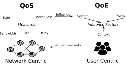
While network performance is typically expressed by QoS met-rics, QoS and QoE represent fundamentally different concepts that can influence each other; QoS represents anetwork centricview whereas QoE represents auser centricview (see Figure 2). QoE depends on a multidimensional perceptual space that includesi)

system influence factors (e.g., QoS measures, transport protocols, or device specific parameters), ii)human influence factors (e.g., mood, personality traits, or expectations), andiii)contextual

fac-tors (e.g., location, task, or costs). For an extensive discussion on factors influencing QoE, we refer to [7]. These features are not necessarily independent of each other and do not always have clear mappings, e.g., users tend to give different opinion scores for the same stimulus, e.g., depending on mood, expectation, and mem-ory. While some QoE influence factors include QoS metrics (e.g., packet loss), QoE depends on a larger set of influence factors that cannot be derived from QoS metrics and requires new measures.

To quantify the users’ perception of the quality of (network) plications, QoE metrics have been defined and standardized for ap-plications such as VoIP, Video, Web, etc. These metrics are rooted in psychological tests that involved human subjects in the metric

construction phase. In theapplication phase, however, they allow automatic quality assessments without user involvement;i.e., con-clusions on user-experience can be drawn from testbed evaluations

without costly user involvement. This is an appealing property as it enables the automatic exploration of a large state space that in-volves a significant number of different workload and buffer size configurations incontrolled experiments. While desired, involv-ing human subjects is time intensive and thus requires only a small set of conditions to be tested in order to be economically feasi-ble. However, insights obtained in this paper allow sub-sampling of this large state space and therefore enable subjective tests to be conducted in future work.

We base our QoE evaluation on standardized and widely used QoE metrics for quality assessment. Since the metrics depend on the applications, we refer the reader to the corresponding section for a discussion of the used metrics.

5.

METHODOLOGY

We use a testbed driven approach to study the impact of buffer sizes on the user perception (QoE) of common types of Internet applications:i)Voice over IP,ii)RTP/UDP video streaming as used in IPTV networks, andiii)web browsing.

5.1

Testbed Setup

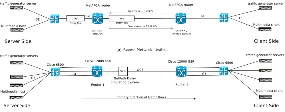
We consider two scenarios:i)an access network andii)a back-bone or core network. Each scenario is realized in a dedicated testbed as shown in Figure 3 (a) and (b). We use a testbed setup to have full control over all parameters including buffer sizes and generated workload.

(a) Access Network Testbed

(b) Backbone Network Testbed

Figure 3: Access and backbone network testbeds used in the study

case we configured the bandwidth and the delays of all links sym-metrically. For the access network we use an asymmetric bottle-neck link. In the backbone case we only consider data transfers from the servers to the clients. For the access network we also include data uploads by the clients—as they mainly triggered the bufferbloat debate [19].

The access network testbed, see Figure 3a, consists of two Gi-gabit switches, four quadcore hosts equipped with 4 GB of RAM and multiple Gigabit Ethernet interfaces. Moreover, two hosts are equipped with a NetFPGA 1 Gb card each. The hosts are connected via their internal NICs to the switch to realize the client/server side network. The NetFPGA cards run the Stanford Reference Router software and are thus used to realize the bottleneck link. Thus the NetFPGA router and the multimedia hosts are located on the same physical host. As the NetFPGA card is able to operate indepen-dent of the host, it does not impose resource contention. The right NetFPGA router acts as the home router, aka DSL modem, whereas the left one acts as the DSLAM counterpart of the DSL access net-works. To capture asymmetric bandwidth of DSL we use the hard-ware capabilities of the NetFPGA card to restrict the uplink and downlink capacities to approximately 1 respectively 16 Mbit/s. We use hardware to introduce a 5 ms respectively 20 ms delay between the client (server) network and the routers. The 5 ms delay corre-sponds to DSL with 16 frame interleaving or to the delays typical for cable access networks [10]. The 20 ms account for access and backbone delays. While we acknowledge that delays to different servers vary according to a network path, a detailed study of path delay variation is beyond the scope of this paper. This is also the reason we decided to omit WiFi connectivity which adds its own variable delay characteristics due to layer-2 retransmissions. In-stead, we focus on delay variations induced by buffering.

To be able to scale up the background traffic to the backbone net-work, see Figure 3b, we include eight hosts, four clients and four servers. Each has again a quadcore CPU, 4 GB of RAM, and multi-ple Gigabit Ethernet network interfaces. The client/server networks are connected via separate Gigabit switches, Cisco 6500s, to back-bone grade Cisco 12000GSR routers. Instead of using 10 Gbit/s and soon to be 100 Gbit/s interfaces for the bottleneck link, we use an OC3 (155 Mb/s nominal) link. The reason for this is that we wanted to keep the scale of the experiments reasonable, this

in-cludes,e.g., the tcpdump files of traffic captures. Moreover, scaling down allows us to actually experience bufferbloat given the avail-able memory within the router. We use multiple parallel links be-tween the hosts, the switch, and the router so that it is possible for multiple packets to arrive within the same time instance at the router buffer. With regards to the delays we added a NetPath delay box with a constant one-way delay of 30 ms to the bottleneck link. 30 ms delay roughly corresponds to the one-way delay from the US east to the US west coast. We again note, that the path delays in the Internet are not constant. However, variable path delays are be-yond the scope of this paper. Instead we focus on delay variability induced by buffering. Moreover, we eliminate most synchroniza-tion potential by our choice of workload (see § 5.2).

To gather statistics and to control the experiments we always use a separate Ethernet interface on the hosts as well as a separate phys-ical network (not shown).

5.2

Traffic Scenarios

We use the Harpoon flow level network traffic generator [38] to create a number of congestion scenarios which range from no background traffic (noBG) to fully overloading (short-overload) the bottleneck link. Congestion causes packets from both the back-ground traffic as well as the application under study to be queued or dropped just before the bottleneck link. Depending on the fill grade of the buffer, the size of the buffer, and the link speed, this will increase the RTT accordingly (see Table 2). Overall, we use 12 scenarios for the access testbed and 6 for the backbone. We consider more for the access to distinguish on which links (i.e., up-stream, downup-stream, or both) the congestion is subjected to.

Testbed Name Flow Interarrival File Size # Sessions Concurrent Link Utilization [%] Packet Description

Distribution Distribution Up Down Flows Mean Sd Loss [%]

Up Down Up Down Up Down

A

cc

es

s

noBG — — — — — — — — — — — No bg. traffic

short-few exp-a weibull

1 — 98.9 0.3 0.7 0.1 34.7 0 Upstream

1 8 95 8.5 5.6 15.2 58.6 0.7 Bidirectional

— 8 27.8 44.1 13.7 25.1 1.4 3 Downstream

short-many exp-a weibull

1 — 98.9 0.3 0.7 0.1 33.1 0 Upstream

1 16 93.3 10.7 4.3 20.1 60.9 1.3 Bidirectional

— 16 53.8 78.7 12.8 23.5 4 4.5 Downstream

long-few — infinite

1 — 99 0.2 0.7 0.0 1 0 Upstream

1 8 71.9 83.1 8.9 12.6 41.7 0.6 Bidirectional

— 8 39.5 99.9 1.9 0.6 0.1 0.5 Downstream

long-many — infinite

8 — 98.9 0.3 0.7 0.0 14.4 0.0 Upstream

8 64 83.8 61.8 11.2 26.4 60.7 0.2 Bidirectional

— 64 68.5 99.6 3.9 4.9 0.03 9.3 Downstream

B

ac

k

b

o

n

e

noBG — — — — — — — — No bg. traffic

short-low exp-b weibull — 3∗10 18 16.5 11.6 0

short-medium exp-b weibull — 3∗30 49 49.5 18.8 0

short-high exp-b weibull — 3∗60 206 98 6.5 0.2

short-overload exp-b weibull — 3∗256 2170 99.7 2.2 5.2

long — infinite — 3∗256 675 99.7 0.1 3.8

Table 1: Workload configuration for both testbeds, where the flow interarrival time distributions are specific to the access and backbone testbed; exp-a has a mean of 2 sec and exp-b a mean of 1 sec. The file size distribution is defined as weibull(shape=0.35, scale=10039), resulting in a mean flow size of 50 KB. The number of parallel flows at the bottleneck link is shown by their mean. Link utilization and loss measures are obtained for buffers configured according to the BDP.

For scenarios with long-lived flows (long) we use flows of in-finite duration. In this case the link utilization is almost indepen-dent of the number of concurrent flows. For long-tailed file sizes the workload of each scenario is controlled via the number of con-current sessions that Harpoon generates. A session in Harpoon is supposed to mimic the behaviour of a user [38] with a specific in-terarrival time, a file size distribution, and other parameters. We used the default parameters except for the file size distribution. In addition, we rescaled the mean of the interarrival time for the ac-cess network, as Harpoon’s default parameters are geared towards core networks with a larger number of concurrent flows. To impose different levels of congestion we adjusted the number of sessions for the backbone scenario to result in low, medium, high, and over-load scenarios which correspond to link utilizations as shown in Table 1. For the access network we distinguish between few and many concurrent flows which results in medium and high load for the downstream direction and high load for the upstream, see Ta-ble 1.

We checked that all hosts are using a TCP variant with window scaling. Due to the Linux version used the background traffic uses TCP-Reno in the backbone and TCP BIC/TCP CUBIC for the ac-cess. However, note that this does not substantially impact the QoE results as the applications VoIP and video rely on UDP and the Web page is relatively small. Moreover, since the results are consistent it suggests that using a TCP variant optimized for high latency does not change the overall behavior even when the buffers are large.

5.3

Buffer Configurations

One key element of our QoE study is the buffer size configura-tions. Buffers are everywhere along the network path including at the end-hosts, the routers, and the switches. The most critical one is at the bottleneck interface, the only location where packet loss occurs. Therefore we focus on these and rely on default parameters for the others. For the bottleneck we choose a range of different buffer sizes, some reflect existing sizing recommendations, some are chosen to be small other large in order to capture extremes. Ta-ble 2 summarizes the buffer size configuration in terms of number of packets and shows the corresponding queuing delays.

For the access network we choose buffer sizes of powers of two, ranging from 8 to 256 packets. 256 is the maximum supported

Access Backbone

Buffer Uplink Downlink Buffer

Size Delay Scheme Delay Scheme Size Delay Scheme

(Pkts) (ms) (ms) (Pkts) (ms)

8 98 ≈BDP 6 min 8 0.6 ≈TinyBuf

16 198 12 28 2.2 Stanford

32 395 24 749 58 BDP

64 788 49 ≈BDP 7490 580 10×BDP

128 1,583 97

256 3,167 max 195 max

Table 2: Buffer size configurations and corresponding maximum queuing delays for both testbeds (full sized packets).

buffer size by the Stanford Reference Router software. For our choice of an asymmetric link (recall 1 Mbps uplink/16 Mbps down-link) the bandwidth-delay product (BDP) corresponds to roughly8

and64packets, respectively. Since this set of buffer sizes yields delays up to buffer bloat, we consider the buffer configurations to approximate home router behaviour.

For the backbone network we usei)the same minimum buffer size of 8 packets, which resembles the TinyBuffer scheme [17], depending on the largest congestion window achieved by the work-loads. In addition, we useii)749 full-sized packets which corre-sponds to the BDP formula given an RTT of 60 ms,iii)28 packet which corresponds to the Stanford scheme [9],i.e., BDP/√n, where

n = 3∗256is the maximum number of concurrent for short-low,short-medium,short-high, andlong(see Table 1), andiv) 10×BDP packets an excessive buffering scheme.

6.

QOS: BACKGROUND TRAFFIC

To highlight the potential importance of the buffer configuration on latencies, network utilization, and packet loss—the typical QoS values—we start our study with a detailed look at the background traffic. While the story is relatively straight forward for the back-bone scenario, and captured in Table 1, it is more complicated for the access network as the number of concurrent flows is smaller and there are subtle interactions between upstream and downstream.

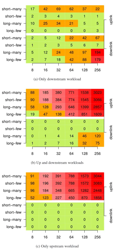
utilization statistics of the FPGA cards. Figure 4 shows the corre-sponding mean delays as heatmaps. We use three different heatmaps: one each for downstream/upstream workload only and one for com-bined up- and downstream workload. Each heatmap has two subareas— one for upstream at the top and one for downstream at the bottom. Each heatmap cell show the mean delay for a specific buffer size configuration and workload scenario, measured over two hours. The color of the heatmap cells correspond to categories of the ITU-T Recommendation G.114 which classifies delays based on their potential to degrade the QoE of interactive applications: green (light gray) is acceptable, orange (medium gray) problematic, and red (dark gray) causes problems.

In principle, we see that larger buffers sizes can increase the de-lays significantly independent of the workload. For the downlink direction the maximum delay is less than200ms. However, this can differ for the uplink direction. In particular, we observe delays of up to three seconds for larger–over-sized–buffers when the up-stream is used for the uplink direction. This is almost independent of the workload! Overall, these delays are consistent with observa-tions by Gettys [6] which started the bufferbloat discussion.

Given these high latencies, we investigate the link utilization. Figure 5 shows a boxplot of the link utilization for the various buffer sizes in the scenario with simultaneously downloads and up-loads (bidirectional workup-loads). The left/right half focuses on the downlink/uplink utilization. The uplink utilization is almost 100% while the downlink utilization ranges from 20% to 100%. Consis-tent with related work, we see that very small buffers can lead to underutilization while very large buffers can lead to large delays.

Comparing these link utilizations to those with no upstream work-load (not shown) we find that, for bidirectional workwork-loads, the buffer configurations below the BDP do not always fully utilize the down-link direction. Buffer sizes that correspond to the BDP yield full downlink utilization in the absence of upload workload, but not with concurrent download and upload activities. This phenomena can be explained by the queuing delay introduced by bloated uplink buffers thatvirtuallyincrease the BDP thus rendering the downlink under-buffered. Related work coined the problem of bidirectional TCP flows that influence each otherdata pendulum[23]. In contrast to related work, our analysis highlights interdependencies between buffers and suggests that buffers should not be sized independent of each other.

The phenomena of low link utilization can be mitigated by counter-intuitively “bloating” the downlink buffer. Considering the delays observed in Figure 4b, the BDP increases beyond the initial buffer size of 64 to 835 full sized packets. Note, that we can get full link utilization for buffers of smaller than 835 packets as we have a suf-ficient number of concurrent flows active.

In summary, the latency introduced by the buffers in home routers, aka, the uplink, might not only i) harm real-time traffic applica-tions (due to excessive buffering), but also ii) drastically reduce TCP performance (due to insufficient buffering) in case of bidirec-tional workloads in asymmetric links. In effect it invalidates the buffer dimensioning assumptions due to the increase in RTT.

7.

VOICE OVER IP

We start our discussion of application QoE with Voice over IP (VoIP). In IP networks speech signals can be impaired by QoS pa-rameters (e.g., packet loss, jitter, and/or delay), talker echo, codec and audio hardware related parameters, etc. Regarding QoS param-eters, packet losses directly degrade speech quality as long as for-ward error correction is not used as is typical today. Network jitter can result in losses at the application layer as the data arrives after its scheduled playout time. Moreover, excessive delays impairs any

2 5 1 2 0 10 2 17 7 12 2 5 0 25 3 42 18 24 3 12 0 34 4 69 42 48 5 22 0 21 3 62 88 97 6 42 0 5 1 37 179 194 7 67 3 5 1 22

8 16 32 64 128 256

long−few long−many short−few short−many long−few long−many short−few short−many do wnlink uplink

(a) Only downstream workload

1 0 0 0 19 58 90 88 2 1 0 0 47 128 188 185 7 4 0 0 138 293 384 380 16 14 0 0 412 646 774 771 32 46 0 0 851 1399 1545 1538 75 120 0 0 1609 2857 3066 3023

8 16 32 64 128 256

long−few long−many short−few short−many long−few long−many short−few short−many do wnlink uplink

(b) Up and downstream workloads

0 0 0 0 52 96 98 91 0 0 0 0 123 184 196 192 0 0 0 0 227 348 392 391 0 0 0 0 450 665 788 788 0 0 0 0 870 1282 1572 1573 0 0 0 0 1858 2448 3083 3044

8 16 32 64 128 256

long−few long−many short−few short−many long−few long−many short−few short−many do wnlink uplink

(c) Only upstream workload

Figure 4: Mean queuing delay (in ms) for the access networks testbed with different buffer size (x-axis) and workload (y-axis) configurations. Delays that significantly degrade the QoE of in-teractive applications (ITU-T Rec. G.114) are colored in red.

bidirectional conversation as it changes the conversational dynam-ics in turn taking behavior.

7.1

Approach

8 16 32 64 128 256 8 16 32 64 128 256 0

20 40 60 80 100

Buffer size (in packets)

Link utilization (%)

downlink uplink

Figure 5: Link utilization for an asymmetric access link with var-ious buffer sizes. The uplink and the downlink are simultaneously congested by 8 and 64 long-lived TCP flows, respectively.

recording of a male or female Dutch speaker, encoded with G.711.a (PCMA) narrow-band audio codec, and lasts for eight seconds. Each of the 20 samples is automatically streamed, using the PjSIP library, over our two evaluation testbeds, see § 5 and subjected to the various workloads. PjSIP uses the typical protocol combination of SIP and RTP for VoIP. We remark that we do not consider other situational factors such as the users’ expectation (e.g., free vs. paid call) [31] which can also affect the perceived speech quality (see § 4). For the VoIP QoE assessment, we separately evaluate speech signal degradations and conversational dynamics, using two widely used and standardized QoE models: PESQ and E-Model. Individ-ual scores are combined to the final QoE score.

Speech signal degradations. To assess the speech quality of

each received output audio signal, relative to the error-free sample signal, we use the Perceptual Speech Quality Measure (PESQ) [2] as standardized model. PESQ takes as input both the error-free audio signal and the perturbed audio signal, and computes the QoE scorez1. Note that whilez1isinfluencedby loss and jitter, the QoE

estimation issignal basedandnot a function of QoS parameters. The influence of loss and jitter onz1can therefore not be quantified.

Conversational dynamics. The PESQ model only accounts for

the perceived quality when listening to a remote speaker but does not account for conversational dynamics,e.g., for humans taking turns and/or interrupting each other. This can be impaired by ex-cessive delays and thus can degrade the quality of the conversation significantly [31, 26, 34, 35]. Thus, according to the ITU-T recom-mendation G.114 one-way delays should be below 150 ms (or at most 400 ms).

Therefore, we measure the packet delay during the VoIP calls. We now use the delay impairment factor of the ITU-T E-Model [3] to get a scorez2. We remark that even thoughz2is computed using

a standardized and widely used model, it is subject to an intense de-bate within the QoE literature as there is a dispute about the impact of delay on speech perception [26, 34, 16]. Among the reasons is that the delay impact depends on the nature of the conversational task (e.g, reading random numbers vs. free conversation) as well as the level of interactivity required by the task [26]. Thus, there can be mismatches between the quality ratings of the E-Model and tests conducted with subjects.

Overall score. The range of the scorez1, which captures loss

and jitter, is[1,5]. We remap it to[0,100]according to [41]. The range of the scorez2, capturing the delay impairment, is[0,100].

Note, the semantics ofz1andz2are reversed: a large value forz1

reflects an excellent quality; however, a large value forz2reflects

a bad quality, and vice-versa. We combine the two scores to an

MOS

1 2.6 3.1 3.6 4 4.3 5

Very Satisfied Satisfied Some Users Satisfied Many Users Dissatisfied Nearly All Users Dissatisfied

Not Recommended

(a) G.711 (PCMA audio codec).

MOS

1 2 3 4

5 Excellent

Good

Fair

Poor

Bad

(b) Video & Web

Figure 6: MOS scales used in this paper

overall one as follows:z= max{0, z1−z2}. Thus, ifz1is good

(i.e., due to negligible loss and jitter), but thez2 is bad (i.e., due

to large delays), then the overall scorez is low, reflecting a poor quality and vice-versa. Finally, we mapzto the MOS scale[1,5]

according to the ITU-T recommendation P.862.2, see Figure 6a; in the end, low values correspond to bad quality and high values to excellent quality.

7.2

Access networks results

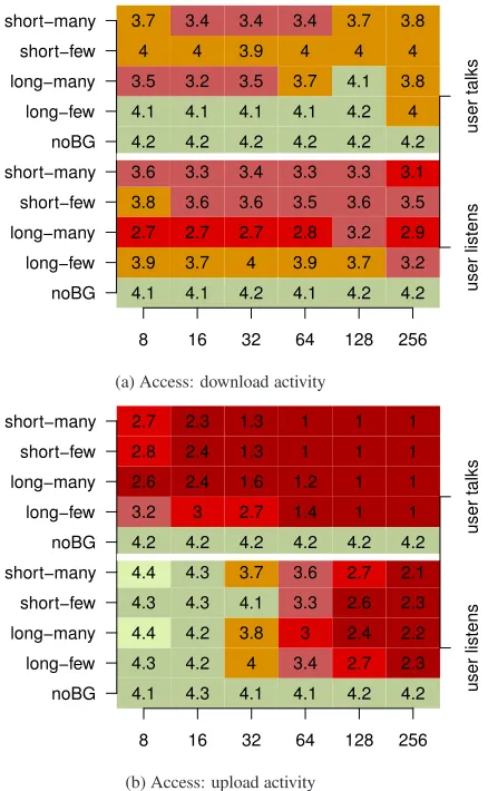
Figures 7a and 7b show heatmaps of the median call quality (MOS) for the access networks. Each cell in the heatmap shows the median MOS of 200 VoIP calls (each speech sample is send 10 times) per buffer size (x-axis) and workload scenario (y-axis) com-bination. The heatmap is colored according to the color scheme of Figure 6a. The heatmap is divided into two parts (i) when user talks (upper part) and (ii) when the user listens to the remote speaker (bottom part).

The baseline results, namely the ones without background traffic are shown in the bottom row of each heatmap part, labelednoBG. They reflect the achievable call quality of the scenarios. As all of them are green, we can conclude that in principle each scenario supports excellent speech quality and that any impairment is due to congestion and not due to the buffer size configuration per se.

Download activity. Figure 7a focuses on the scenarios when

there is congestion in the downlink. As there is no explicit work-load in the uplink, one may expect that only the “user listens” part is effected but not the “user talks” part. This is only partially true as the “user talks” part of the heatmap shows deviations of up to0.8

MOS points from the baseline score. These degradations are ex-plained by the substantial number of TCP ACK packets, reflected by higher link utilizations (not shown). Recall, the uplink capacity is 1/16th only of the downlink capacity.

The degradations in “user listens” part of the heatmap are, as expected, more pronounced then for the “user talks” part. How-ever, there are also significant differences according to the work-load and the buffer configurations. For instance, with buffers sizes of 64 packets thelong-manyworkload yields a median MOS of

4.1 3.9 2.7 3.8 3.6 4.2 4.1 3.5 4 3.7 4.1 3.7 2.7 3.6 3.3 4.2 4.1 3.2 4 3.4 4.2 4 2.7 3.6 3.4 4.2 4.1 3.5 3.9 3.4 4.1 3.9 2.8 3.5 3.3 4.2 4.1 3.7 4 3.4 4.2 3.7 3.2 3.6 3.3 4.2 4.2 4.1 4 3.7 4.2 3.2 2.9 3.5 3.1 4.2 4 3.8 4 3.8

8 16 32 64 128 256

noBG long−few long−many short−few short−many noBG long−few long−many short−few short−many user listens user talks

(a) Access: download activity

4.1 4.3 4.4 4.3 4.4 4.2 3.2 2.6 2.8 2.7 4.3 4.2 4.2 4.3 4.3 4.2 3 2.4 2.4 2.3 4.1 4 3.8 4.1 3.7 4.2 2.7 1.6 1.3 1.3 4.1 3.4 3 3.3 3.6 4.2 1.4 1.2 1 1 4.2 2.7 2.4 2.6 2.7 4.2 1 1 1 1 4.2 2.3 2.2 2.3 2.1 4.2 1 1 1 1

8 16 32 64 128 256

noBG long−few long−many short−few short−many noBG long−few long−many short−few short−many user listens user talks

(b) Access: upload activity

Figure 7: VoIP Access: Median Mean Opinion Scores (MOS) for voice calls with different buffer size (x-axis) and workload (y-axis) configurations. The heatmaps for the access networks include in-bound calls (user listens) and outin-bound calls (user talks).

We conclude that the level and kind of workload has a more sig-nificant effect than buffer size.

Upload activity. Figure 7b focuses on the scenarios when there

is congestion on the uplink. According to the above reasoning one would therefore only expect degradations for the “user talks” part. This is not the case. The MOS in the “user listens” part of the heatmap decreases by0.5to2from the baseline results for all sce-narios with buffer sizes≥ 64. The reason for this is that the de-lays added by the excessive buffering in the uplink also degrade the overall score due to the delay impairment factorz2. Since this

factor expresses the conversational quality, it does not only effect the “user talks” but also the “user listen” part sent over the (non-congested) downlink.

Excessive delays added by the buffers also explain the significant degradation of MOS values from4.2to1−1.4for the “user talks” part. Due to the congestion, packet loss is also significant for all scenarios. This is why the best MOS value is limited to3.2even for short buffer configurations.

In the context of the bufferbloat discussion, Figure 7b corrobo-rates that excessive buffering in the uplink yields indeed bad qual-ity scores. Reducing the buffer sizes results in better MOS and contributes to mitigate the negative effects of the large delays

in-4.4 4.4 4.4 3.5 1.5 2.8 4.4 4.4 4.2 3.5 1.7 2.7 4.4 4.4 4.3 3.5 1.5 3.2 4.4 4.4 4.2 3.1 1.2 1.6

8 28 749 7490

noBG short−low short−medium short−high short−overload long

Figure 8: VoIP Backbone: Median Mean Opinion Scores (MOS) for voice calls with different buffer size (x-axis) and workload (y-axis) configurations.

troduced by the uplink buffer,e.g., the difference in the MOS for an inbound audio can be as high2.5points (long-manyworkload).

Combined upload and download activity. Scenarios (plot

not shown) with upload and download congestion show similar re-sults to scenarios with only uploads. Here as well the delays intro-duced by the uplink buffer dominate in both “user talks” and “user listens” parts. However, with combined upload and download ac-tivity, the “user listens” is slightly more degraded than with only upload activity. The reason for this is additional background traffic in the downlink that interacts with the voice call. For instance, with buffers configured to16packets, thelong-fewshows an additional degradation of0.8MOS points (thus mapping to a different rating scale).

Limiting access congestion by isolating VoIP calls in a separate QoS class—as often implemented for ISP internal services but not Internet-wide—is therefore a good strategy.

7.3

Backbone networks results

Similar to the access network scenario, we show the voice quality in the backbone network scenario as a heatmap in Figure 8. The heatmap shows the median MOS for unidirectional audio from the left to the right side of the topology per buffer size (x-axis) and workload scenario (y-axis). Each cell in the heatmap is based on 2000 VoIP calls. Here, each speech sample is send 100 times which is possible as the total number of scenarios is smaller. As in the access network scenario, the bottom row labelnoBGshows the baseline results for an idle backbone without background traffic.

While the effects of the buffer size are less pronounced, the na-ture of the background traffic (longvs. short-*) and the link uti-lization (short-lowtoshort-overload) are more significant. The type of workload can drastically degrade the quality score. Con-cretely, low to medium utilization levels as imposed by the sce-nariosshort-lowandshort-medium, respectively, are close to the baseline results. In contrast, more demanding workloads such as the scenariosshort-highandlong, leading to higher link utiliza-tions, and result in more than1point reductions in the MOS scale. Further, the aggressiveness of the workload further decrease the quality; the median MOS for theshort-overloadworkload is1.5

and thus significantly lower than forshort-highandlongthat also lead to high link utilizations.

configura-tion. However, buffer configuration larger than the BDP, i.e, 7490 packets, lead to excessive queueing delays. As in the access net-work scenario, excessive delays lead to significant quality degra-dations of thez2delay impairment component. For example, the

scores corresponding to the scenarios longand short-overload

workloads have MOS values of almost half of their counterpart with the BDP configuration.

7.4

Key findings for VoIP QoE

We find that VoIP QoE is substantially degraded when VoIP flows have to compete for resources in congested links. This is particu-larly highlighted in the backbone network scenario, where low to medium link utilizations yields good QoE and high link utilization (>98%) degrade the QoE. In the case of the latter, the congestion leads to insufficient bandwidth on the bottleneck link that affects the VoIP QoE.

For access networks we show that, due to the asymmetric link capacities, the different audio directions can yield different QoE scores. For instance, in one direction (e.g., user talks) the speech quality might be acceptable, while it is impaired for the other (e.g., remote speaker talks) or vice-versa. Moreover, the speech quality is much more sensitive to congestion on the upstream direction than the downstream one. Due to the light queueing delays introduced by bloated buffers in the uplink, maintaining a conversation can be challenging in the presence of uplink congestion.

For both access and backbone networks, configuring small buffers can results in better QoE. However, our results highlight that this may not suffice to yield “excellent” quality ratings. Thus, we advo-cate to use QoS mechanisms to isolate VoIP traffic from the other traffic. This is already common for ISP internal services but not for ISP external services.

8.

RTP VIDEO STREAMING

Next, we explore the quality of video streaming using the Real-time Transport Protocol (RTP) which is commonly used by IPTV service providers. RTP streaming can be impaired by packet loss, jitter, and/or delay. Again packet losses directly degrades the video as basic RTP-based video streamingtypicallydoes not involve any means of error recovery. Network jitter and delays result in simi-lar impairments as with voice and include visual artifacts or jerky playback. However, they depend on the concrete error concealment strategy applied by the video decoder.

8.1

Approach

We chose three different video clips from various genres as ref-erence. Each video has a length 16 seconds. They are chosen to be representative of various different kinds of TV content and vary in level of detail and movement complexity. Thus, they result in different frame-level properties and encoding efficiency;A)an in-terview scene, B)a soccer match, and C)a movie. Each video is encoded using H.264 in SD (4 Mbps) as well as HD (8 Mbps) resolution. Each frame is encoded using 32 slices to keep errors localized. This choice of our encoding settings is motivated by our experiences with an operational IPTV network of a Tier-1 ISP.

We use VLC to stream each clip using UDP/RTP and MPEG-2 Transport Streams. Without any adjustment VLC tries to transmit all packets belonging a frame immediately. This leads to traffic spikes exceeding the access network capacity. In effect VLC and other streaming software propagate the information bursts directly to the network layer. As our network capacity, in particular for the access, is limited we configured VLC to smooth the transmission rate over a larger time window as is typical for commercial IPTV vendors. More specifically, we decided to use a smoothing interval

1 0.47 0.41 0.47 0.44 1 0.55 0.46 0.56 0.53 1 0.47 0.4 0.48 0.43 1 0.56 0.46 0.56 0.51 1 0.47 0.4 0.48 0.42 1 0.55 0.47 0.56 0.5 1 0.47 0.41 0.48 0.41 1 0.56 0.45 0.56 0.48 1 0.47 0.42 0.48 0.45 1 0.56 0.47 0.56 0.48 1 0.47 0.44 0.48 0.46 1 0.56 0.51 0.57 0.48

8 16 32 64 128 256

noBG long−few long−many short−few short−many noBG long−few long−many short−few short−many SD HD

(a) Access: download activity

1 1 0.95 0.46 0.4 0.38 1 0.99 0.58 0.52 0.45 0.44 1 1 0.95 0.47 0.4 0.38 1 0.99 0.58 0.53 0.45 0.44 1 1 0.88 0.48 0.41 0.4 1 1 0.59 0.56 0.46 0.45 1 1 0.88 0.49 0.46 0.48 1 1 0.59 0.58 0.54 0.56

8 28 749 7490

noBG short−low short−medium short−high short−overload long noBG short−low short−medium short−high short−overload long SD HD (b) Backbone

Figure 9: Median MOS (color) and SSIM (text) for HD and SD RTP video streams with different buffer size (x-axis) and workloads (y-axis).

(1second) that ensures that the available capacity is not exceeded in the absence of background traffic. The importance of smoothing the sending rate is often ignored in available video assessment tools such as EvalVid, making them inapplicable for this study.

We note that Set-top-Boxes in IPTV networks often use propri-etary retransmission schemes that request lost packets once [24]. Due to the unavailability of exact implementation details we do not account for such recovery. Our results thus present a baseline in the expected quality; however, systems deploying active (retransmis-sion) or passive (FEC) error recovery can achieve higher quality.

We use two different full-reference metrics, PSNR and SSIM, to compute quality scores from the original and the perturbed video stream. While not considered as QoE metric, PSNR (Peak Signal Noise Ratio) enables a quality ranking of the same video content subject to different impairments [43, 27]. However, it does not nec-essarily correlate well with human-perception in general settings. SSIM (Structural SIMilarity) [47] has been shown to correlate bet-ter with human perception [48]. We map PSNR and SSIM scores to quality scores according to [49].

8.2

Access network results

(x-axis) and workload (y-axis) combination. Each cell shows the median SSIM score and is colored according to the corresponding MOS score (see Figure 6b); a SSIM score of 1 expresses excel-lent video quality, whereas 0 expresses bad quality. The upper and the bottom parts of the heatmap correspond to the results of HD and SD video streams, respectively. We omit quality scores ob-tained for the PSNR metric as they yield predicted scores similar to those obtained by SSIM. Also, as we focus on IPTV networks where the user consumes TV streams, no video traffic is present in the upstream. For this reason, we only show results for workloads congesting the downlink.

To show the achievable quality for all buffer size configurations in the absence of background traffic, we show baseline results in rows labelednoBG. In these cases, the video quality is not de-graded due to the absence of congestion.

In the presence of congestion, however, the SD video quality is severely degraded, expressed by a “bad” MOS score. This holds regardless of the workloads and the buffer configuration; the link utilization by all of the workloads cause video degradation due to packet loss in the video stream. We observe that even a low packet loss rate can yield low MOS estimates. Moreover, much higher loss rates (one order of magnitude bigger) can yield the same estimates. For instance, although both scenarios,long-fewandlong-many, have a similar SSIM and MOS score for buffers sized to 256 and 8 packets respectively, they show different packet loss rates of0.5% and12.5%.

In comparison to the SD video, degradations in HD videos are less pronounced although, in some cases, the packet loss rate is higher. For instance, the packet loss rate for HD and SD video streaming is, with thelong-fewworkload and buffers sized to 256 packets, 2.6% and 1.3% respectively. However, the HD video stream obtains a better MOS score. This interesting phenomena can be explained by the higher resolution and bit-rate of HD video streams, which reduce the visual impact of artifacts resulting from packet losses during video streams.

In the case of UDP video streaming in access networks, what matters is the available bandwidth, not the buffer size. Moreover, even though buffers regulate the trade-off between packet losses and delay, they have limited influence on the quality from the per-spective of an IPTV viewer.

8.3

Backbone network results

Similar to the previous access network scenario, we show the video quality scores obtained for the same video C as a heatmap in Figure 9b, both for SD and HD resolution. Each cell of the heatmap shows the median SSIM score and is colored according to the corresponding perceptive MOS score (see Figure 6b). As in the previous scenario, the video was sent 50 times per buffer size (x-axis) and workload (y-(x-axis) configuration. We omit PSNR quality scores as they are similar to the SSIM quality scores.

As in the access network scenario, the bottom row labelednoBG

shows the baseline results for an idle backbone without background traffic. Similarly, workloads that do not fully utilize the bottleneck link,i.e.,short-low, lead to optimal video quality, as expressed by an SSIM score of 1. The reason is that the available capacity in the bottleneck link allows streaming the video without suffering from packet losses.

First quality degradations are observable in theshort-medium

scenario, where the quality decreases with increasing link utiliza-tion. In this scenario, workloads achieve full link utilization for 749/7490 buffers more often than for the 8/28 buffer configura-tions. It results in higher loss rates for the video flows lowering

the quality and is more pronounced for the HD videos which have higher bandwidth requirements.

Workloads that sustainably utilize the bottleneck link,i.e., short-high,short-overload, andlong, yield bad quality scores due to high loss rates. These scenarios provide insufficient available band-width to stream the video without losses. Increasing the buffer size helps to decrease the loss rate, leading to slight improvements in the SSIM score.

Comparing the obtained quality scores among the three different videos leads to minor differences in quality scores. These ences result from different encoding efficiencies that cause differ-ent levels of burstiness in the streamed video. However, the quality scores of all video clips lead to the same primary observation: qual-ity mainly depends on the workload configuration and decreases with link utilization. Increasing the buffer size helps to lower the loss rate and therefore to marginally improve the video quality.

8.4

Key findings for RTP video Quality

when the bottleneck link has sufficient available capacity to stream the video, the video quality is good, andii)otherwise the quality is bad. In between, if the background traffic utilizes the link only temporarily, the video quality is sometimes degraded. This results in an overall degradation that increases with link utilization. Us-ing HD videos yields marginally better quality scores even though they use higher bandwidth. We find that the influence of the buffer size is marginal as delay does not play a major role for IPTV. What mainly matters is the available bandwidth. We did not include qual-ity metrics relevant for interactive TV or video-calls. We further note that our results represent a baseline quality achievable without error recovery. Error recovery (e.g., retransmissions) will increase the overall quality.

9.

WEB BROWSING

We next move to web browsing, our last application under study. The web browsing experience (WebQoE) can be quantified by two main indicators [14]. One is thepage loading time(PLT), which is defined as the difference between a Web page request time and the completion time of rendering the Web page in a browser. Another is the time for the first visual sign of progress. In this paper we consider PLT of information retrieval tasks, for which there exists an ITU QoE model (i.e., G.1030 [5]) to map page loading times to user scores.

We note that WebQoE does not directly depend on packet loss ar-tifacts, but rather on the completion time of underlying TCP flows. Thus, factoring in various workloads and buffer sizing configura-tions—which influence the TCP performance—is particularly rele-vant for understanding WebQoE from a network only perspective. Given that the PLT as measured in a browser can be approximated from flow completion times as parameter, is sometimes considered as a QoS parameter. Since the applied G.1030 model logarithmi-cally maps PLT to QoE, it can be misbelieved QoS parameters can (always) be mapped to QoE. We therefore note that other QoE mod-els are of higher complexity as different input parameter are used that cannot be directly derived from a QoS parameters, e.g., speech signals as used in Section 7.

9.1

Approach

as shown in Figure 6b). This mapping uses six seconds as the max-imum PLT,i.e., mapping to a “bad” QoE score. The minimum PLT—mapping to “excellent”—is set to 0.56 (0.85) seconds for ac-cess (backbone) scenario, due to different RTTs.

We remark that WebQoE research has advanced beyond factors captured in the applied ITU G.1030 [5] model. This concerns the impact of distraction factors such as noise or traffic on quality per-ception [21], task and content dependent factors [39], or task com-pletion times and loading pattern [40]. These advances have, how-ever, not yet converged to an revised model that is applicable in this study. Beyond additional factors, WebQoE research addresses the need for interactive web use that goes beyond information re-trieval tasks which follow request response pattern [15]. We remark that no QoE models fully addresses interactive web usage (such as AJAX requests), which is why we must leave this aspect for fu-ture work. For the information retrieval scenario considered in this section, however, recent findings suggest the logarithmic depen-dency of waiting time and QoE [15, 40]—as used in applied G.1030 model—to remain valid. We thus stick to using ITU Recommen-dation G.1030 [5] as the current standard for assessing WebQoE.

To measure the PLT’s, we consider a single static web page, lo-cated in one of the testbed servers, and consisting of: one html file, one CSS file, and two medium JPEG images (sized to15,5.8,

30, and30KB, respectively). The web page is loaded within 14 RTTs, including the TCP connection setup and teardown. Choos-ing a relatively small web page size was inspired by the frequently accessed Google front page designed to quickly load. To retrieve this web page we use thewgettool which measures the transfer time.wgetis configured to sequentially fetch the web page and all of its objects in a single persistent HTTP/1.0 TCP connection with-out pipelining. We point with-out that, as static web pages have constant rendering times, it suffices to rely onwgetrather than on a specific web browser.

To further analyze the page retrieval performance, we rely on full packet traces capturing the HTTP transactions. We analyze the loss process of the captured TCP flows using thetcpcsmtool estimating retransmission events. We further measure the RTT during each experiment. We denote PLTs as RTT dominated if a significant portion of the PLT consists of the RTT component expressed by

14∗RT T. Similarly, we denote PLTs as loss dominated if the increase in PLT can be mainly attributed to TCP retransmissions.

9.2

Access network results

Figures 10a and 10b show heatmaps of the median web browsing quality (MOS) for the access network. Each cell in the heatmap shows the median PLT of 300 web page retrievals per buffer size (x-axis) and workload scenario (y-axis) combination. The heatmap is colored according to Figure 6b.

The baseline results, namely the ones without background traffic, are shown in the bottom row of each heatmap part, labelednoBG. The fastest PLT that can be achieved in this testbed is≈ 0.56s. As all of the cells are green (light gray), we can conclude that in principle each scenario almost supports excellent browsing quality and that any impairment is due to congestion. In this respect, it turns out that, even without background traffic, the WebQoE can be degraded by (too) small buffers,e.g., 8 packets. Due to packet losses causing retransmissions, the PLT is increased to1second thereby changing the user perceived quality.

Download activity. Figure 10a focuses on the scenarios when

there is congestion on the downlink. For theshort-fewscenario the downlink is not fully utilized, thus most scores do not devi-ate much from the baseline results. With this type of moderdevi-ate workload browsing can benefit from the capacity of large buffers

1s 0.8s 3.8s 0.8s 1.4s

0.6s 0.9s 3.7s 0.8s 1.3s

0.6s 1.1s 3.4s 0.8s 1.1s

0.6s 1.4s 4.4s 0.7s 1s

0.6s 2.1s 4.9s 0.6s 1s

0.6s 3.1s 5.8s 0.6s 1.2s

8 16 32 64 128 256

noBG long−few long−many short−few short−many

(a) Access: only download activity

1s 1.3s 8.2s 4s 7s

0.6s 2.1s 6.2s 7.1s 8.3s

0.6s 3.1s 3.9s 10.1s 11.4s

0.6s 5.1s 7.4s 13s 14s

0.6s 8.9s 14.6s 16.6s 16.1s

0.6s 20.5s 24.4s 18.7s 19.2s

8 16 32 64 128 256

noBG long−few long−many short−few short−many

(b) Access: only upload activity

Figure 10: WebQoE Access: Median MOS (color) and page load-ing times (text) with different buffer size (x-axis) and workloads (y-axis).

to absorbe transient bursts and reduce packet losses. For instance, configuring the buffers size to 256 packets reduces the PLTs to the baseline results (as opposed to PLTs of0.8s for the smallest buffer configuration). Likewise, for theshort-manyscenario, which in-volves more competing flows and imposes a higher link utilization, big buffers generally reduce PLTs. As the queueing delays for these scenarios are not excessive,i.e., they are bounded by 192 ms, see Table 2, large buffers do in fact improve the QoE by limiting the loss rate.

Bufferbloat is visible for thelong-fewscenario, where the me-dian PLT increases with the buffer size, as the PLT is dominated by RTTs caused by large queueing delays. As for the previous sce-nario, the effects of various buffer sizes are clearly perceived by the end-user (yet in a different manner).

In contrast, the buffer size does not change the WebQoE in the

long-manyscenario. The larger number of competing flows re-duces the per-flow capacity and lets the PLT increases beyond the users’ acceptance threshold. Therefore, the perceived QoE, in con-trast to the previous configuration, can not be improved by adjust-ing the buffer size. Nevertheless, from a QoS perspective, config-uring an appropiate buffer size can let web pages to load2seconds faster. This is not as straightforward since it involves considering the tradeoff between small buffers (packet losses) and large buffers (combined effect of packet losses and large RTTs).

Upload activity. Figure 10b focuses on the scenarios when

min-0.9s 0.8s 0.9s 1.3s 3.4s 5s

0.8s 0.8s 1s 1.3s 3.5s 4.8s

0.8s 0.8s 0.8s 1.5s 4.5s 5.9s

0.8s 0.8s 0.8s 1.6s 9.5s 9.2s

8 28 749 7490

noBG short−low short−medium short−high short−overload long

Figure 11: WebQoE Backbone: Median MOS (color) and page loading times (text) with different buffer size (x-axis) and work-loads (y-axis).

imum for every buffer size configuration of the scenarios short-many, short-few, and thelong-many. The only scenario where the browsing experience is slightly more acceptable is the long-fewscenario if buffers are small. Such configuration reduces the median PLT from 20 to 1.3 seconds, which maps to afairquality rating.

From a QoS perspective, the figure shows that the PLT and the buffer size are strongly correlated to the QoE. A wise decision on the dimensioning of the buffers can reduce the PLT from24.4to

3.8seconds (long-many). However, and in line with the previous observations, such reductions do not generally suffice to change the user perceived (bad) quality.

Combined upload and download activity. In the case of

work-loads in both, the uplink and downlink direction (not shown), the QoE is dominated by the upload activity. However, due to lower

overalllink utilization and shorter queueing delays (see § 6), the median PLT are less than for the scenarios involving only uploads. The resulting scores generally map tobadquality scores; only the

long-fewworkload shows better QoE for buffers≤128packets.

9.3

Backbone networks results

The median PLT and the corresponding QoE scores in the back-bone setup are shown as a heatmap in Figure 11. As in the ac-cess scenario, the heatmap shows buffer sizes on the x-axis and the workload configuration on the y-axis. Each cell is colored accord-ing to the MOS scale from Figure 6b and displays the median PLT of 500 web page retrievals.

The baseline results (noBG) show median page loading times of≈ 0.8seconds. These loading times are mainly modulated by

14×RTT (RTT= 60ms (see § 5.1)) needed to fully load the page (RTT component), making them higher than in the access network scenarios that has lower RTTs. In this scenario, the distribution of page loading times generally yields a slightly better performance for buffer sizes greater than or equal to the BDP; for these buffer configurations web pages load up to 200 ms faster (80th_percentile

not shown in the figure). Theshort-lowscenario yields similar results despite the existence of background traffic.

We observe the first PLT degradations in theshort-medium sce-nario for the 8 and 28 packets buffer configurations. In these cases, PLTs are affected by packet losses causing TCP retransmissions, while the 749 (BDP) and 7490 packet buffers absorb bursts and prevent retransmissions. As in the previous case, web pages load up to 200 ms faster (80th

percentile not shown in the figure). The degradations in PLT are, however, small and only marginally affect the QoE score.

Degradations in theshort-highscenario are twofold; while packet losses mainly affect the QoE for the 8 and 28 packets buffers, queu-ing delays degrade the QoE for the larger buffers. This effect is more pronounced in theshort-overloadandlongscenarios that impose a higher link load. In these scenarios, the degradations for the 8 and 28 buffers are mainly caused by packet losses. The 749 and especially the large 7490 buffer affected flow by intro-ducing significant queueing delays; while the RTT doubles for the 749 buffer configuration, it increases by a factor of 10 for the 7490 buffer. Comparingshort-overloadtolongfor the 8, 28 and 749 buffer size yields a higher number of retransmissions in thelong

scenario, degrading the PLT. Concerning the PLT, short buffers of 8 and 28 packets show faster PLT for the short-high, short-overload, andlongscenarios. However, improvements in the PLT do not help to generally improve the QoE as the PLTs are already high, causing bad QoE scores.

Our findings highlight the trade-off between packet loss and queue-ing delays. While larger buffers prevent packet losses and therefore improve the PLT in cases of less utilized queues/links, the intro-duced queuing delays degrade the performance in scenarios of high buffer/link utilization. In the latter, shorter buffers improve the PLT by avoiding large queueing delays, despite the introduced packet losses. The “right” choice in buffer size therefore depends on the utilization of the link and the buffer.

9.4

Key findings for WebQoE

Our observations fall into two categories: i)When the link is low to moderately loaded, larger buffers (e.g., BDP or higher) help minimizing the number of retransmissions that prolong the page transfer time and thus degrade WebQoE.ii)When the link utiliza-tion is high, however, this increases RTT and thus the page transfers become RTT dominated. Also, loss recovery times increase. There-fore, smaller buffers yield better WebQoE despite a larger number of losses.

However, the impact of the buffer size on the QoE metric page loading time is ultimately marginal, although the QoS metric page loading time sees significant improvements. While this may seem weird at first, let us consider a twofold improvement of the page loading time from 9 seconds to 5 seconds. This improvement is large for the QoS metric, but it is insignificant for the QoE metric, as both 9 and 5 seconds map to “bad” QoE scores regardless the QoS performance.

10.

SUMMARY & DISCUSSION

The goal of our work is to elucidate the open problem of proper buffer sizing and to pave the way for more informed sizing deci-sions. In this respect, this paper presents the first comprehensive study of the impact of buffer sizes onQuality of Experience. By this we complement a large body of related work on buffering with a first look at factors relevant to end-user experience. This is a relevant view since it has implications for network operators and service providers, and by extension, device manufacturers.

To tackle this problem, we first evaluate the impact of buffering in the wild using a large data set from a major CDN that serves for a large number of Internet users (80M IPs from 235 countries). Our analysis shows that buffering is likely to be prevalent on a large scale. We also observe a rather modest amount of potential buffer bloat. This motivates our further evaluation of buffer sizing includ-ing the impact of very large buffers,i.e., buffer bloat.