The stochastic volatility Markov functional model

(1)

warwick.ac.uk/lib-publications

A Thesis Submitted for the Degree of PhD at the University of Warwick

Permanent WRAP URL:

http://wrap.warwick.ac.uk/91418

Copyright and reuse:

This thesis is made available online and is protected by original copyright.

Please scroll down to view the document itself.

Please refer to the repository record for this item for information to help you to cite it.

Our policy information is available from the repository home page.

(2)

The Stochastic Volatility Markov-functional Model

by

Chuan Guo

Thesis

Submitted to the University of Warwick

for the degree of

Doctor of Philosophy

Depatment of Statistics

(3)

List of Tables

2.1 Examples of short rate models . . . 15

4.1 Calibration performance for implied volatilities (%) of the ATM caplets 99

4.2 Calibration performance for implied volatilities (%) of the ATM co-terminal swaptions . . . 100

4.3 Scenarios for the SV MFM. . . 101

4.4 Calibration performance for one-step correlation of LIBORsCorr(ln(Li_T

i+

θi), ln(Li_T+1_i₊₁+θi+1)) under SV MFMs with different scenarios . . . . 101

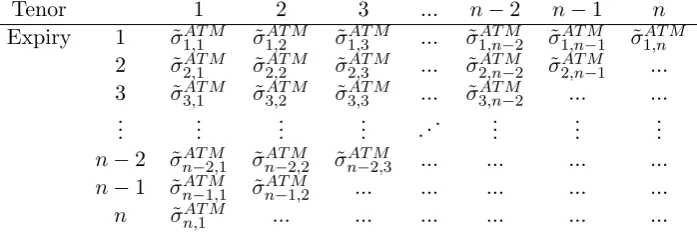
5.1 ATM implied volatilities in the swaption matrix linked to the

Hull-White driver. . . 114 5.2 ATM implied volatilities in the swaption matrix linked to the one

step covariance driver and the SABR driver. . . 115

5.3 The expressions for vegasvi,k for a particulariof a Bermudan

swap-tion under swap MFMs whereθi := deσ

Berm i,n+1−i

deσ

AT M i,n+1−i

. . . 120

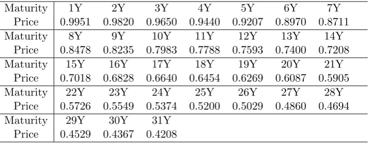
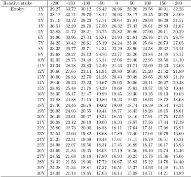
5.4 Initial zero-coupon bonds on 11 March 2015. . . 122 5.5 Implied volatilities (%) of the co-terminal (31Y) swaptions against

expiry and relative strike (bp) to the ATM on 11 March 2015 . . . . 123

5.6 Implied volatilities (%) of the caplets against expiry and relative strike (bp) to the ATM on 11 March 2015 . . . 124

5.7 Implied volatilities (%) of the ATM swaptions against expiry and

tenor (1Y - 10Y) on 11 March 2015 . . . 125 5.8 Implied volatilities (%) of the ATM swaptions against expiry and

tenor (11Y - 20Y) on 11 March 2015 . . . 126

5.9 Implied volatilities (%) of the ATM swaptions against expiry and tenor (21Y - 30Y) on 11 March 2015 . . . 127

(7)

5.11 The prices of the Bermudan swaption under different MFMs with

notionalN = 100 million. . . 128 5.12 The difference between the price for the Bermudan swaption produced

by different MFMs and the SV MFM (I) measured by total vega. . . 129

5.13 The prices of the new Bermudan product under different MFMs with notionalN = 100 million. . . 132 5.14 The difference between the price for the new Bermudan product

(8)

List of Figures

5.1 The sum of the vegas Pn+1−i

k=1 vi,k for i= 1, ...,30 of the Bermudan

swaption under the different MFMs. . . 135

5.2 The sum of the vegasPn+1−i

k=1 vi,k fori= 1, ...,30 of the new

(9)

Acknowledgments

First and foremost, I would like to thank my supervisor Dr Jo Kennedy for her

support and patience. Without her help and suggestions throughout the last four

years, this thesis would not have been possible. Thank you so much Jo.

Second, I thank my review panel, Dr Anastasia Papavasiliou and

Profes-sor Gareth Roberts, for your valuable advice and feedback of my presentation and

reports.

Third, I would like to thank Duy Pham and Jaka Gogala for sharing with me

your C++ code and all discussions we have. Many thanks go to the other members

in the Statistics department. I have really enjoyed this friendly environment in the

department.

Fourth, I am grateful to the scholarship I have received from the university

of Warwick. I cannot focus all my mind on this thesis without the financial support.

Thanks for providing me this valuable opportunity to study here.

I am also grateful to my friends who accompany me throughout the PhD

period. Jian and Bing, I will never forget the basketball time every weekend and

your brain teasers. I also want to thank my roommates Dave and Matt. Thank you

for improving my English and all the joy we had together.

Finally, I would like to thank my parents and my wife for their support and

(10)

Declarations

I declare that this thesis is based on my own work. The thesis is original except

where specified by the references. The thesis has not been submitted for any other

degree at any other university. The material in this thesis has not been submitted

(11)

Abstract

In this thesis we study low-dimensional stochastic volatility interest rate mod-els for pricing and hedging exotic derivatives. In particular we develop a stochastic volatility Markov-functional model. In order to implement the model numerically, we further propose a general algorithm by working with basis functions and condi-tional moments of the driving Markov process. Motivated by a data driven study, we choose a SABR type model as a driving process. With this choice we specify a pre-model and develop an approximation to evaluate conditional moments of the SABR driver which serve as building blocks for the practical algorithm.

Having discussed how to set up a stochastic volatility Markov-functional model next we study the calibration of a LIBOR based version of the model with the SABR type driving process. We consider a link between separable SABR LIBOR market models and stochastic volatility LIBOR Markov-functional models. Based on the link we propose a calibration routine to feed in SABR marginals by calibrating to the market vanilla options. Moreover we choose the parameters of the SABR driver by fitting to the market correlation structure.

We compare the stochastic volatility Markov-functional model developed in the thesis with one-dimensional (non-stochastic-volatility) swap Markov-functional models in terms of pricing and hedging Bermudan type products. By doing so we investigate effects of correlation structure, implied volatility smiles and the intro-duction of stochastic volatility on Bermudan type products.

(12)

Chapter 1

Introduction

In this thesis we work in the area of interest rate models. There are three popular categories of term structure models for pricing and hedging interest rate derivatives

in practice. They are short rate models, market models and Markov-functional

models. Among them, short rate models (1970s) are the earliest term structure models. They were very popular and are still used nowadays in practice because of

their tractability. In a short rate model the dynamics of the short rate, which is an

instantaneous spot rate and not observable in the market, is specified. So they are low-dimensional models. In LIBOR (swap) market models (1997), the dynamics of

a set of contiguous market observable forward rates - LIBORs (swap rates) - are

specified. Market models are high-dimensional models even when driven by a single Brownian motion. An advantage for market models is that they allow for calibration

to the well-known Black’s formula for vanilla options. A Markov-functional model

(2000) is specified via the dynamics of a Markov process. In a Markov-functional model the zero coupon bonds, which are underlying assets in the interest rate

mar-kets, are a function of the Markov process. Besides the above interest rate models,

Heath-Jarrow-Morton framework (1992) models the entire forward rate curve di-rectly and, without appropriate conditions being imposed on the volatility of the

instantaneous forward rates, this framework can be non-Markovian and infinite

di-mensional.

In this thesis we focus on Markov-functional models. Markov-functional

mod-els were introduced by Hunt et al. [37]. Usually in a Markov-functional model, the

economy is driven by a low-dimensional Markov process which is referred to as the driving process, and the zero coupon bonds are a function of the driving process. In

(13)

con-trast, in a Markov-functional model, the functional forms for zero-coupon bonds can

be determined numerically by feeding in marginal distributions of a set of contiguous LIBORs or swap rates. In principle given a driving process, any marginal

distribu-tions can be fed into the model. As a result Markov-functional models have more

calibration advantage than market models since in addition to the Black’s formula Markov-functional models allow for calibration to implied volatility smiles/skews of

vanilla options by feeding in appropriate marginal distributions of LIBORs (swap

rates). In fact there is a link between Markov-functional models and market models. Bennett and Kennedy [7] compared a one-factor separable LIBOR Market model to

a one-dimensional Markov-functional model driven by a Gaussian process calibrated

to the Black’s formula for caplets, and the two models turned out to be very similar numerically.

The vast majority of the research on all these term structure models is in

the non-stochastic volatility setting, and this is especially true for Markov-functional models where we have not found any article in the literature on the stochastic

volatil-ity extensions. One main contribution we make in this thesis is the development of

a stochastic volatility Markov-functional model.

Typically in a valuation model, the evolution of the underlying asset prices is

described via a diffusion process. In a non-stochastic volatility model the volatility of the underlying asset, i.e. the coefficient of the diffusion term, is a deterministic

function of the current asset level and time. For example the volatility function of the

Black-Scholes [8] model is a constant. In contrast, in a stochastic volatility model, the volatility function is driven by its own SDE and at least one extra (correlated)

Brownian motion. There are a number of empirical studies showing that volatility is

stochastic in reality in the interest rate markets; see [15], [49] and references therein. But does this justify adding the extra complexity to a model for derivative pricing

and hedging? Without stochastic volatility the set of distributions we can get for

the underlying asset is constrained and does not match reality. In particular it does not have heavy enough tails. Dupire [19] introduced a local volatility model and

pointed out that a suitable choice of the local volatility function allows one to fit

the marginal distribution of the underlying asset derived from the market prices of European options. However as Hagan et al. [31] pointed out, without stochastic

volatility the joint distributions of the underlying asset are not a good reflection

of reality. The joint distributions of the underlying assets are very important for pricing and hedging path dependent derivatives such as Bermudan swaptions in

practice.

(14)

volatility. See, for example, [24], [49], [18], [12], [5] and references therein. After

that, over the last two decades, many studies about stochastic volatility extensions to LIBOR market models have been developed. See, for example, [65], [55], [61],

[23] and references therein. But market models are high dimensional so that it

is difficult to implement their stochastic volatility version. These articles about stochastic volatility extensions focused on the development and calibration of the

models.

In this thesis we study stochastic volatility Markov-functional models. We provide a background introduction in Chapter 2. The basic interest rate products

and derivatives are introduced briefly. We also give an outline of the popular term

structure models appearing in the literature.

In Chapter 3, we begin with a review of Markov-functional models with

a Gaussian driving process introduced by Hunt, Kennedy and Pelsser [37]. We

introduce an algorithm for implementation of Markov-functional models with a Gaussian driver. We then develop a stochastic volatility Markov-functional model.

Kaisajuntti and Kennedy [44] identified a two-dimensional SABR type model as an

appropriate choice for the level of rates by investigating market data. This moti-vates us to choose a SABR type model as the driving process. The two-dimensional

algorithm for the specification of a Markov-functional model with a Gaussian driver and additive pre-model discussed in [38] relies heavily on the Gaussian

assump-tion. This algorithm can not be used for the stochastic volatility Markov-functional

model since we do not have explicit knowledge of the transition density function of the SABR driving process. To implement the model numerically, we propose an

algorithm which works with conditional moments of the driver distribution based

on an approximation introduced by Kennedy et al. [47]. By working with basis functions and conditional moments of the driving Markov process, we calculate and

store three (conditional) expectations which can be seen as building blocks. The

model can be implemented based on these building blocks. The algorithm we de-velop is not specific to a Gaussian driving process and could be modified to apply

to all one- and multi-dimensional Markov-functional models.

In Chapter 4, we study the calibration of the stochastic volatility LIBOR Markov-functional model developed in Chapter 3. As we discussed earlier, the

specification of a driving process is separated from the marginal distribution of

LIBORs at their setting dates in the associated forward measure, which can be seen as an unusual feature for interest rate models. Thus the calibration issue

for the stochastic volatility LIBOR Markov-functional model involves choosing the

(15)

the input prices of the set of digital caplets which will be fed into the model.

The separation of a driver and marginals provides more flexibility for a Markov-functional model. But this may also cause an issue. A mismatch of a

driving process and marginals could potentially lead to nontransparent dynamics of

forward LIBORs and could result in an unstable evolution of the implied volatility surface. This potential issue has been pointed out by Andersen and Piterbarg [5]

who argue that a non-parametric formulation of the marginal distribution for

LI-BORs may result in unrealistic evolution of the volatility smile through time. On the other hand, Bennett and Kennedy [7] showed that a LIBOR Markov-functional

model with a Gaussian driver together with the Black’s formula for (digital) caplets

is numerically similar to the one-factor separable LIBOR market model. Gogala and Kennedy [29] extended the above link to a more general local-volatility case.

Based on this link, the authors propose an approach for choosing an appropriate

combination of a driving process and (digital) caplet prices, and such a combination leads to desirable dynamics of future implied volatilities. In Chapter 4 we

con-sider a separable SABR-LIBOR market model and expect that it is similar to the

stochastic volatility Markov-functional model with a SABR driver together with a SABR marginals. Based on this link the intuition behind the SDEs of the separable

SABR-LIBOR market model can be applied to the corresponding stochastic volatil-ity LIBOR Markov-functional model. This gives us an appropriate combination of

the driver and marginals. Based on this link we develop a calibration routine to

feed in SABR marginals by calibrating to market prices of caplets or swaptions. Moreover the parameters for the SABR driving process can be chosen by

calibrat-ing to the market implied correlations. A numerical investigation of the calibration

performance is also given.

In Chapter 5, we compare the stochastic volatility Markov-functional model

developed in Chapter 3 with one-dimensional swap Markov-functional models in

terms of pricing and hedging a Bermudan swaption and a new Bermudan product, which has similar features but simpler payouts than callable range accruals. We

consider different combinations of the specifications of driving process and marginals.

By comparing their Bermudan prices and vega profiles, we investigate impacts of smiles, correlation structure and stochastic volatility on Bermudan products.

The numerical results show that the mean reversion parameter of the mean

reversion and Hull-White drivers, which determines the auto-correlations of the driver, has a large effect on prices of Bermudan products. By comparing the

Hull-White Markov-functional model together with log-Normal marginals to the local

(16)

marginals, it turns out that the smile impact on the price of Bermudan products

is very small. In order to study the impact of stochastic volatility on the prices of Bermudan products, we compare the one step covariance swap

(non-stochastic-volatility) functional model with the stochastic volatility swap

Markov-functional model. The results show that the introduction of stochastic volatility has a small influence on a Bermudan swaption but has a significant impact on the

new Bermudan product. This suggests using a stochastic volatility model for

pric-ing the new Bermudan product. No other papers we have found have identified a product for which stochastic volatility should be added to a term structure model.

The vega profiles of Bermudan products indicate a fundamental difference

between the mean reversion driver, which is “parameterized by expiry”, and the other driving processes “parameterized by time”. By “parametrization by expiry”

we mean that the auto-correlations of the driver are fully determined by input

pa-rameters. This implies that once input parameters have been fixed, any change in market implied volatility has no effect on the auto-correlations of the driver and

therefore the swap rates at their setting dates, which is inconsistent with what we

observed in the market. In contrast, for parametrization by time, the correlations of the driver are sensitive to market implied volatilities. Thus any change in market

implied volatilities will result in a change in the correlations of the driver. This leads to a fundamental difference in the vega profiles between parametrizations by expiry

and by time. For non-stochastic volatility models this behaviour is well-known to

practitioners and is analysed in [48] for one dimensional Markov-functional models with the Black’s formula. We find by introducing stochastic volatility, the row sum

of vegas is decreased in comparison to the one step covariance Markov-functional

model but vega profiles of the two models are still very similar. This means that the introduction of stochastic volatility does not materially alter the hedging behaviour.

This finding is significant for practitioners wanting to use stochastic volatility

mod-els.

Chapter 6 compares Quasi-Gaussian models and Markov-functional models

in terms of specification and calibration. These classes of models are two of the

most popular low-dimensional term structure models in practical use but there are no studies in the literature which compare them theoretically or numerically. A

Quasi-Gaussian model can be seen as a separable Heath-Jarrow-Morton model while

a Markov-functional model with a Gaussian driver and log-Normal marginals is found to be numerically similar to the separable LIBOR market model. In order to

gain insight into the relationship between these models we study a Quasi-Gaussian

(17)

essential difference between the non-stochastic volatility versions of the models lies

in the copula of the driving processes and that the Markov-functional framework offers much flexibility in matching the choice of copula for the driver to reality.

These two models both allow for stochastic volatility versions and we also consider

(18)

Chapter 2

Interest rate markets and

models

In this chapter we provide an overview of the interest rate markets and models. We

will introduce notation and set up a foundation for the thesis. In Section 2.1 we

introduce the main interest rate products. In Section 2.2 we give a brief outline of the popular term structure models. We will assume that the reader has knowledge

of pricing via an equivalent martingale measure and application of the fundamental pricing formula for various choices of numeraires. This background can be found in

[38] and [46].

2.1 Interest rate markets

In this section we introduce briefly the interest rate products in the market. We

first introduce some basic instruments that are liquid in the interest rate markets.

We then proceed to some common interest rate options which are relevant to the thesis. The material in this section is from [38].

2.1.1 Basic instruments

In this subsection we will introduce zero-coupon bonds (ZCBs), forward rate agree-ments (FRAs) and interest rate swaps. Throughout this thesis we assume that the

tenor structure is given by

0 =T0< T1 < ... < Tn+1 (2.1)

(19)

We start with underlying assets in the interest rate markets - zero coupon

bonds. A zero-coupon bond with maturity time T is a contract that guarantees its holder to be paid one unit of currency at time T. The contract value at timet≤T is denoted byDtT. The dependence ofDtT on the maturity dateT is known as the

term structure of ZCBs at timet.

LIBOR stands for London Interbank Offered Rate. We can define a forward

LIBOR through a forward rate agreement. A forward rate agreement is an

agree-ment between two counterparties to exchange cash payagree-ments at some specified date in the future. At the maturity Ti+1,i= 1, ..., n, a fixed payment N αiK, where K

is the fixed rate andN is notional amount, is exchanged against a floating payment N αiLi_T_i, where Li_T_i is the spot LIBOR with expiration date Ti and maturity date

Ti+1 defined by

Li_T_i = 1−DTiTi+1 αiDTiTi+1

.

Following a replicating portfolio argument, we have that the time-t value of this FRA is given by

Vt=N DtTi −N(1 +αiK)DtTi+1.

The forward LIBORLi_t, at timet, is defined as the fixed rateK such that the time-t value of the FRA is zero. By letting Vt = 0, the forward LIBOR Lit at time t that

expires atTi and matures at Ti+1 is given by

Li_t= DtTi−DtTi+1 αiDtTi+1

, t≤Ti, (2.2)

fori= 1, ..., n.

Remark 1. The value of the forward LIBORLi₀,i= 1, ..., n, seen today is assumed to be given in the market. But the value of the forward LIBOR Li_t, i= 1, ..., n, at some future timetis a random variable. Later we will introduce interest rate models for the forward LIBOR processesLi for i= 1, ..., n. The same remark also applies to the forward swap rate below.

An interest rate swap, or swap for short, is an agreement between two

coun-terparties to exchange a series of cashflows on pre-agreed dates in the future. There are two kinds of swaps: payers swap and receivers swap. Let us consider a payers

(20)

floating legN αsLsTs at each payment date fors=i, ..., i+j−1. A receivers interest

rate swap has a reversed cashflows. The time-tvalue of the above fixed leg is given by

V_{F XD}i,j (t) =N KP_ti,j, (2.3)

where

P_ti,j :=

i+j−1 X

k=i

αkDtTk+1.

The expression Pi,j is referred to as the present value of a basis point or PVBP for short. Following a replicating portfolio argument, the time-tvalue of the above floating leg is given by

V_{F LT}i,j (t) =N(DtTi−DtTi+j).

It follows that the time-tvalue of the above interest rate swap is given by

V_Swapi,j (t) =τ[V_{F LT}i,j (t)−V_{F XD}i,j (t)]

=τ N[DtTi−DtTi+j−KP

i,j

t ], (2.4)

where τ = −1 leads to a receivers swap and τ = 1 leads to a payers swap. The forward swap rateyi,j_t is defined as the value ofKsuch that the time-tvalueV_Swapi,j (t) of the swap is zero. Thus we have that

y_ti,j = DtTi−DtTi+j

P_ti,j , t≤Ti. (2.5)

If we substitute equation (2.5) back into (2.4), we have the more usual expression

for the value of an interest rate swap:

V_Swapi,j (t) =τ N[P_ti,j(yi,j_t −K)].

2.1.2 Interest rate options

In this subsection we introduce some interest rate options that are relevant to the thesis. These options are caplets (floorlets), vanilla swaptions1, digital caplets

(floor-lets) and PVBP-digital swaptions.

(21)

A caplet and floorlet can be seen as an option on an FRA with the payoffs

V_capleti (Ti+1;K) =N αimax(LiTi−K,0)

and

V_{f loorlet}i (Ti+1;K) =N αimax(K−LiTi,0)

respectively at time Ti+1 whereN is the notional and K is the strike. In order to price such an option in a complete arbitrage-free model, we apply the fundamental

pricing formula. In particular given some equivalent martingale measure M

corre-sponding to the numeraire M, today’s value of the caplet with strike K is given by

V_capleti (0;K) =M0EM[

N αi(LiTi −K)

+

MTi+1 ].

In order to calculate this price we have to choose a numeraire M and a model for the LIBOR Li in the measure M. Suppose we work with the forward measure Fi+1 associated with the numeraireD.,Ti+1. It follows from equation (2.2) that the LIBORLi is a martingale in the forward measureFi+1. Suppose we modelLi by a

driftless log-Normal process under the forward measureFi+1

dLi_t=σi_tLi_tdW_ti+1,

for some deterministic functionσi and a Brownian motion Wi+1 under the forward measure. This yields the following well-known Black’s formula introduced by Black [9]

V_capleti (0;K) =D0Ti+1EFi+1[N αi(L

i Ti−K)

+_] _(2.6)

=αiN D0Ti+1(L

i

0Φ(d1)−KΦ(d2)) (2.7)

where

d1 =

ln(Li₀/K) ˜ σ√Ti

+ 1 2˜σ

p

Ti, (2.8)

d2 =d1−˜σ p

Ti (2.9)

˜ σ2 = 1

Ti

Z Ti

0

(22)

and Φ(·) is the cumulative normal distribution function. Similarly, we have the

following Black’s formula for a floorlet with strikeK:

V_{f loorlet}i (0;K) =αiN D0Ti+1(KΦ(−d2)−L

i

0Φ(−d1)).

We now define the implied volatility of a caplet. Given the market price ˜

V_capleti (0;K) of the caplet struck at the strikeK, the implied volatility of this caplet is defined as the volatility ˜σ such that

˜

V_capleti (0;K) =αiN D0Ti+1(L

i

0Φ(d1)−KΦ(d2))

whered1andd2 are given by equations (2.8) and (2.9) respectively. In financial mar-kets the market prices of vanilla options are quoted in terms of implied volatilities.

In the interest rate markets implied volatilities are commonly observed to represent a shape of skew or smile as a function of strike. However the above log-Normal

assumption of Li implies that the implied volatilities show a flat line with respect to strike i.e. the function ˜σ(K) is always a constant. In order to capture implied volatility skews or smiles, a number of models have been developed. We will return

to this topic in the later chapters.

We now consider vanilla swaptions. A vanilla swaption is an option on an interest rate swap. It gives its holder the right, without any obligation, to enter

into an interest rate swap. According to the underlying interest rate swap there are

two types of swaptions: receivers swaption and payers swaption. For the receivers swaptions, upon exercise the option holder enters a swap in which he receives a

fixed strike rate K and pays the floating rate; a payers is the reverse. So the payoff of a payers swaption with strikeK on an interest rate swap with expiry dates Ti, Ti+1, ..., Ti+j−1 and maturity datesTi+1, Ti+2, ..., Ti+j is given by

V_sptioni,j (Ti;K) = max{N P_Ti,j_i(y_Ti,j_i −K),0},

whereN is the notional andK is the strike.

Following a similar explanation and assuming a driftless log-Normal process

foryi,j under the swaption measureSi,j associated with the numeraire Pi,j, we can

obtain the following Black’s formula for a vanilla swaption

V_sptioni,j (0;K) =P₀i,jESi,j[N(y

i,j Ti −K)

+_]

(23)

where

d1=

ln(yi,j₀ /K) ˜ σ√Ti

+1 2σ˜

p Ti,

d2=d1−σ˜ p

Ti, (2.11)

˜ σ2= 1

Ti

Z Ti

0

(σ_ui)2du.

The explanation for implied volatilities of caplets also applies to vanilla swaptions. The caplets (floorlets) and vanilla swaptions we introduced here are liquidly

traded in the interest rate markets. These options are referred to as vanilla options.

The prices of vanilla options are observable in the market. In practice a valua-tion model for some complex derivatives needs to be calibrated to their relevant

underlying vanilla options.

In what follows, we introduce some less liquid interest rate options traded in the market - digital options. In particular, we introduce two examples that are

most relevant to the thesis: digital caplets (floorlets) and PVBP-digital swaptions. A digital caplet on the LIBORLi _{is an option paying a unit amount at time}

Ti+1 if the LIBORLiTi is above some strike levelK. The payoff at timeTi+1 is given

by

V_digcapi (Ti+1;K) =NI{Li Ti>K},

whereIis indicator function andN is the notional. Taking theTi+1-maturity ZCB

D.,Ti+1 as numeraire and using the same log-Normal model, as we did for caplet, yields

V_digcapi (0;K) =N D0Ti+1Φ(d2),

whered2 is as defined in (2.9).

Remark 2. The payoffs of a caplet and digital caplet are related via the following equation

d

dK(x−K)

+₌₋_I

{x>K}.

In particular differentiate both sides of (2.6) with respect to the strike K, and we have that

dV_capleti (0;K)

dK =−αiV

i

(24)

The implication of the relationship is that knowing the prices of caplet

V_capleti (0;K) for all strike K is equivalent to knowing the prices of digital caplet Vi

digcap(0;K) for allK. This remark also applies to vanilla swaptions and the

corre-sponding PVBP-digital swaptions below.

Remark 3. Given the prices V_digcapi (0;K) of a digital caplet as a function of the strike K≥0, from the fundamental pricing formula we have that

V_digcapi (0;K) =D0,Ti+1EFi+1[NI{Li_Ti>K}] =D0,Ti+1NF

i+1_[_Li

Ti > K],

under the forward measure Fi+1 associated with the numeraire D.,Ti+1. Therefore the prices V_digcapi (0;K) implies the distribution of the LIBOR Li_T

i in the associated

forward measure.

From the above two remarks one can see that the prices V_capleti (0;K) can also determine the distribution of the LIBORLi_T

i in the associated forward measure

Fi+1. This also applies to a vanilla swaption and PVBP-digital swaption where the

distribution of the swap rate at its setting date can be determined in the associated

swaption measure.

A PVBP-digital swaption on the swap rateyi,jwith strikeKhas the following payoff at timeTi

V_digsptioni,j (Ti;K) =N P_Ti,j_iI_{yi,j Ti>K},

whereN is the notional. By assuming a driftless log-Normal process foryi,j under the swaption measure Si,j associated with the numeraire Pi,j, we can also obtain

the following Black’s formula for a vanilla swaption

V_digsptioni,j (0;K) =P₀i,jESi,j[NI{yi,j

Ti>K}]

=N P₀i,jΦ(d2), (2.12)

whered2 is as defined in (2.11).

2.2 Interest rate models

In this section we first discuss the role of valuation models. We then give a brief

(25)

2.2.1 The role of models

In this thesis we use interest rate models to price and hedge exotic interest rate

derivatives. By an exotic derivative we mean one which is not vanilla. Exotic

op-tions are commonly traded over-the-counter so that one needs to find their prices based on interest rate models. To do so a valuation model needs to be calibrated

to other underlying instruments and market information, such as vanilla options,

which are relevant to the exotic option under consideration. By calibration, we mean that the valuation model can reproduce the market prices of the chosen

un-derlying instruments. In this sense valuation models are served as a sophisticated

extrapolation from underlying instruments to produce a model price of an exotic option.

2.2.2 Short rate models

Short rate models are the earliest term structure models. The short ratert at time

tis defined by

rt:=−

∂lnDt,T

∂T |T=t.

The short rateris a hypothetical interest rate which is not observable in the market. Short rate models are specified by describing the evolution of the short rate

drt=µ(rt, t)dt+σ(rt, t)dWtQ, (2.13)

whereWQ is a Brownian motion in the risk-neutral measureQassociated with the

numeraire the bank accountB which satisfies

dBt=rtBtdt.

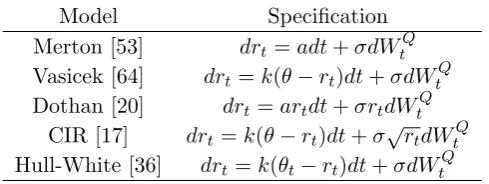
The drift and diffusion functions µ and σ need to be chosen carefully to give the model particular behaviour. Some common examples in the literature are given in

Table 2.1. The parameters of the short rate model (2.13) are chosen by calibrating

the model to the initial term structure and the market prices of vanilla options. The time-tvalueDtT of a ZCB with maturityT is given by

DtT =EQ[e

−RT

t rsds|F_t], (2.14)

where{Ft} is the natural filtration generated by the Brownian motion WQ. From

(26)

Model Specification Merton [53] drt=adt+σdWtQ

Vasicek [64] drt=k(θ−rt)dt+σdWtQ

Dothan [20] drt=artdt+σrtdWtQ

CIR [17] drt=k(θ−rt)dt+σ

√ rtdWtQ

[image:26.595.199.444.106.198.2]

Hull-White [36] drt=k(θt−rt)dt+σdWtQ

Table 2.1: Examples of short rate models

rate markets, can be obtained once we have specified the dynamics of the short rate

rin the risk-neutral measure. Consequently the term structure of ZCBs are specified via the dynamics of the Markov processr. This allows one to price a derivative using an efficient algorithm such as numerical integration or finite-difference method. For

details, the reader is referred to [5]. Since the short rate is not observable in the market, it may result in difficulty of calibrating to the initial term structure and the

market vanilla options.

2.2.3 Heath-Jarrow-Morton models

In a Heath-Jarrow-Morton (HJM) framework [30], the instantaneous forward rate

f(t, T) satisfies the following SDE

df(t, T) =σ(t, T)·( Z T

t

σ(t, u)du)dt+σ(t, T)·dW_tQ, (2.15)

where WQ is an d-dimensional Brownian motion in the risk-neutral measure Q

associated with the numeraire the bank accountB. The instantaneous forward rate f(., T) and the short rate r which can be viewed as an instantaneous spot rate are related via the following equation

f(t, t) =rt.

A short rate model models the dynamics of the short rate r while a HJM model specifies the dynamics of the term structure of instantaneous forward ratesf(., T) for all maturitiesT.

The time-tvalueDtT of a ZCB with maturityT is given by

DtT =e− RT

t f(t,u)du.

From (2.15), one can see that the instantaneous forward rate is specified via the

(27)

model may lead to a known short rate model. We will return to this topic later in

Chapter 6.

2.2.4 Market models

Market models can be divided into two versions: LIBOR market models (LMMs)

and swap market models (SMMs). In a LMM the dynamics of a set of contiguous

forward LIBORsLi,i= 1, ..., n, are specified. LMMs were first introduced by Brace et al. [10], where the dynamics of forward LIBORsLi,i= 1, ..., n, is given by

dLi_t=−

n

X

j=i+1 ( σ

j tαjLjt

1 +αjLjt

)σ_tiρijLitdt+σitLitdWin+1(t), i= 1, ..., n−1 (2.16)

dLn_t =σ_tnL_tndW_nn+1(t).

where Wn+1 is a (correlated) Brownian motion with dW_in+1(t)dW_jn+1(t) = ρijdt

under the terminal measureFn+1 associated with the numeraire theTn+1-maturity ZCB D.,T n+1, and σti is a deterministic function. For more details about the

spec-ification of the volatility functionσi_t, the reader is referred to [11]. The drift term in the SDE (2.16) is determined by maintaining the arbitrage-free property of the

model.

Following the change of measure technique, we obtain the dynamics of Li under the forward measure Fi+1 corresponding to the numeraire D.,T i+1 which is given by

dLi_t=σ_tiL_tidW_ii+1(t), (2.17)

whereWi+1is a (correlated) Brownian motion under the forward measureFi+1. This

is the case since we can see from the definition of LIBORs that Li _{is a martingale}

in the measure Fi+1 so that Li should be a driftless process. Note that the SDE

(2.17) yields the Black’s formula (2.7) for the prices of caplets. Thus LMMs allow for calibration to the Black’s formula for caplets and floorlets, which is an advantage

for LMMs.

The swap market model is specified by describing the dynamics of a set of contiguous forward (co-terminal) swap rates under the terminal measureFn+1

dyi,n_t +1−i=µi_t(yt)yti,n+1−idt+σtiy i,n+1−i

t dWin+1(t) i= 1, ..., n−1, (2.18)

(28)

where

µi_t(yt) =− n

X

j=i+1

Ψj−_t 1Pˆ_tj,n+1−j Ψi−_t 1Pˆ_ti,n+1−i(

αj−1yj,nt +1−j

1 +αj−1yj,nt +1−j

)σi_tσj_tρij

Ψi_t:=

i

Y

j=1

(1 +αjytj+1,n−j)

ˆ

P_ti,n+1−i := P

i,n+1−i t

Dt,Tn+1 .

By moving to the swaption measureSi,n+1−iassociated with the numerairePi,n+1−i,

the forward swap rateyi,n+1−i _{is given by the following driftless process}

dy_ti,n+1−i =σi_ty_ti,n+1−idW_ii,n+1−i(t),

whereWi,n+1−i is a (correlated) Brownian motion under the measureSi,n+1−i. This

leads to the Black’s formula (2.10) for the prices of vanilla swaptions.

We can see that the drift terms of the SDEs (2.16) and (2.18) are dependent

on forward rates. Consequently a market model, though it is Markovian with respect to all its forward rates, is a high-dimensional model even when driven by only

one Brownian motion. In practice a simulation, such as Monte Carlo methods, is

required for an accurate implementation which is computationally expensive. For more details about the specification, calibration, implementation and applications

of market models, the reader is referred to [58] and [59].

2.2.5 Markov-functional models

Markov-functional models (MFMs) were introduced by Hunt et al. [37]. MFMs

can fit any arbitrage-free formula for caplet or swaption prices which includes the

Black’s formula. A MFM is specified via the SDE for a Markov process under some equivalent martingale measure which is referred to as the driving process or the

driver for short. The driving process can be viewed as modelling the overall level

of interest rates in the economy. The defining characteristic of MFMs is that the underlying assets in the interest rate market - ZCBs prices - are a function of a

Markov process so that the term structure of ZCBs can be specified by describing

the dynamics of the Markov process and the functional forms. Recall that in a short rate model, the prices of ZCBs can be computed via the formula (2.14). In a MFM

(29)

implement the model efficiently because one only needs to track the low-dimensional

Markov process. We will return to this topic later in the next chapter.

Let us conclude this section with a remark. Short rate models and market

models allow for stochastic volatility extensions. See for example [24] and [62].

However there is no research in the literature about stochastic volatility extensions of MFMs. The purpose of this thesis is to study stochastic volatility interest rate

models, and one main contribution we make is the development, calibration and

(30)

Chapter 3

Stochastic volatility

Markov-functional models

3.1 Introduction

In this chapter we consider Markov-functional models introduced by Hunt, Kennedy

and Pelsser [37]. Markov-functional models are interest rate models that allow for calibrating to any arbitrage-free formula for caplet or swaption prices. The

defining characteristic of Markovfunctional models is that the underlying assets

-Zero Coupon Bonds - are a function of a Markov process so that the term structure of zero coupon bonds can be specified by describing the dynamics of the Markov process

and the functional form. If the Markov process is chosen to be low dimensional, it is

possible to implement the model efficiently because one only needs to track the low-dimensional Markov process. The functional form can be determined to fit the prices

of a set of caplets or swaptions by numerical integration. Hunt and Kennedy [38]

applied a low-dimensional Gaussian process as the Markov process and calibrated the Markov-functional model to the Black’s formula for caplets or swaptions. They also

proposed an efficient algorithm to specify the Markov-functional model. Caspers [13]

considered the numerical implementation of a one-dimensional Markov-functional model with a Gaussian driver. Kaisajuntti and Kennedy [45] studied the case when

the Markov process is N-dimensional. Gogala and Kennedy [29] developed a one-dimensional Markov-functional model driven by a non-Gaussian Markov process

and proposed an efficient algorithm to implement the model numerically. Fries and

Eckstaedt [27] studied hybrid Markov-functional models; see also [26] and [28]. In Markov-functional models the functional forms of zero coupon bonds can

(31)

bonds are not given explicitly. This makes Markov-functional models less

transpar-ent in terms of the dynamics of forward rates. Bennett and Kennedy [7] partially tackled this problem. The authors compared a one-factor separable LIBOR market

model with a one-dimensional Markov-functional model driven by a Gaussian

pro-cess together with a log-Normal marginal distributions of LIBORs at their setting dates. The numerical results showed that under a wide range of market conditions

these two models have similar dynamics and Bermudan swaption prices for short

maturities (10 years). For long maturities and high volatilities the similarity begins to break down. This link gives us more understanding and intuition of a

Markov-functional model from the corresponding one-factor separable LIBOR market model.

Gogala and Kennedy [29] extended the above link by concluding that the one-factor separable local volatility LIBOR market model has similar dynamics to the

Markov-functional model with the same local volatility type driver and pricing formula for

caplets.

Over the last two decades many stochastic volatility term structure models

have been proposed e.g. [4], [65], [55], [62], [61], [60], [34] and [33]. The

introduc-tion of stochastic volatility is motivated by the empirical evidence (see [4]) that the volatilities in interest rate option markets possess a random component and Hagan

et al’s [31] argument that the smile dynamics in stochastic volatility models behave more realistically than local volatiliy models. The stochastic volatility interest rate

models mentioned above are all high-dimensional models and need to be

imple-mented by simulation. Thus in practice it is infeasible, from the point of view of banks, to use such models for pricing and especially hedging exotic derivatives.

Andersen and Piterbarg [5] developed a stochastic volatility Quasi-Gaussian

model which is a low-dimensional stochastic volatility term structure model. In this chapter we will develop another low-dimensional stochastic volatility interest

rate model - the stochastic volatility Markov-functional model. As Kaisajuntti and

Kennedy [44] pointed out, a one-factor stochastic process is not enough to cap-ture the overall level of interest rates. The authors identified a SABR type model

as an appropriate choice for the level of rates by investigating market data. This

finding motivates us to develop a stochastic volatility Markov-functional model by taking a SABR model as the driving process to capture the overall level of interest

rates and drive the whole economy. The main challenge for the specification of the

model is that it is hard to obtain the transition density function of the driver. To implement the model numerically, we propose an algorithm which works with

con-ditional moments of the driver distribution based on an approximation introduced

(32)

for the additive pre-model, which relies heavily on the Gaussian assumption, the

algorithm we developed is not specific and could be modified to apply to all one-and multi-dimensional Markov-functional models.

The chapter is organized as follows. In Section 3.2 we revisit the LIBOR and

Swap Markov-functional models with a Gaussian driving process and introduce the numeraire approach to specify the model under the terminal measure. In Section 3.3

we develop a stochastic volatility Markov-functional model and discuss the numerical

implementation by developing a general algorithm which works with basis functions and conditional moments of the driving Markov process. Moreover the specification

of the driving process as well as the pre-model for the stochastic volatility

Markov-functional model is given. We conclude in Section 3.4.

3.2 Markov-functional models

In this section we review Markov-functional models (MFMs) proposed by Hunt,

Kennedy and Pelsser [37]. First we give a definition of a MFM from Hunt and Kennedy [38] (see also [29] for a generalized definition). We will know some general

properties of a MFM from the following definition but it will not tell us the

spec-ification of a MFM in practice. We will introduce an algorithm to specify a MFM later in the section.

Definition 1. An interest rate model is said to be Markov-functional if there exists some numeraire pair (N,N) and some process x such that:

(P.1) the process x is a Markov process under the measure N.

(P.2) the zero coupon bond prices are of the form

DtT =DtT(xt) 0≤t≤T ≤T∗,

for a finite time horizonT∗ <∞. (P.3) the numeraireN is of the form

Nt=Nt(xt) 0≤t≤T∗.

A MFM is said to be ofd-dimension ifx is ad-dimensional Markov process. We can see from the above definition that the prices of zero coupon bonds (ZCBs),

(33)

it needs to be implemented by simulation. Moreover the existence of a numeraire

pair ensures that all the numeraire-rebased ZCBs are martingales in the equivalent martingale measure N. In particular the prices of ZCBs can be obtained by the

martingale property

DtT =NtEN[ 1 NT

|F_t],

where{Ft}is the natural filtration generated by the Markov processxin the measure

NandEN(·) denotes an expectation underN. This ensures that a MFM is arbitrage-free. We will present the numeraire approach to specify a MFM under the terminal

measure, which is an equivalent martingale measure, later in the section.

The above definition is very general. In fact most interest rate models are

included in the category of MFMs according to the above definition. For example

in a short rate model the short rate is taken as the Markov process and ZCBs are some function of it. In a LIBOR market model (LMM) however, the evolution of

a set of contiguous forward LIBORs with different maturities are specified. The

high-dimensional LIBORs process can be seen as the Markov process.

For efficient implementation we commonly use a low-dimensional Markov

process with dimensiond63. A high-dimensional MFM needs to be implemented by simulation such as Monte-Carlo methods which is much slower (see [45] for high-dimensional MFMs). In this thesis we restrict our attention to low-high-dimensional

MFMs. Similar to Market models, there are two common versions of MFMs: LIBOR

MFMs and Swap MFMs. The LIBOR version is set up by feeding in digital caplets prices whereas the swap MFM is specified by fitting PVBP-digital swaptions prices.

In the next two subsections we will introduce the specification of both versions of MFMs under the terminal measure Fn+1 corresponding to the numeraire D.,Tn+1. MFMs can also be developed under the spot measure and details can be found in

[28] and [29].

3.2.1 One-dimensional Markov-functional models: LIBOR version

Before discussing multi-dimensional MFMs, it will be helpful to review the

speci-fication of a one-dimensional LIBOR MFM under the terminal measure using the

numeraire approach. We will specify the model on a grid, which is sufficient for most applications in practice and we can see it later when we use a MFM to price

and hedge Bermudan swaptions. In what follows we first specify the driving Markov

processxand then we determine functional forms of the numeraireDTiTn+1(xTi) by

(34)

Suppose we are given the following Gaussian process x:

dxt=σtdWtn+1, (3.1)

where Wn+1 is a one-dimensional Brownian motion in the terminal measure Fn+1

andσt is a deterministic function. Note that theoretically any diffusion process can

be used as a driver. We choose a Gaussian process as the driving Markov process here for efficient implementation. More details about one-dimensional MFMs driven

by non-Gaussian Markov processes can be found in [29].

Having specified the Markov processx, we now consider the problem of how to find the functional formsDTiTn+1(xTi) for i= 1, ..., n. We proceed by backwards

induction on timeTi. At time Tn+1 by definition we have that

DTn+1Tn+1(xTn+1) = 1.

Assume that we have determinedDTkTn+1(xTk) fork=i+ 1, ..., n+ 1. At timeTi,

by definition, the LIBORLi_T_i is given by

Li_T_i = 1−DTiTi+1 αiDTiTi+1

. (3.2)

It follows from equation (3.2) that the numeraire at timeTi can be expressed as

DTiTn+1(xTi) =

1

b

DTiTi+1(xTi)(1 +αiL

i Ti(xTi))

, (3.3)

where the numeraire-rebased ZCBDb_T_i_T_i₊₁ is defined as

b

DTiTi+1(xTi) :=

DTiTi+1(xTi)

DTiTn+1(xTi)

.

It follows from the martingale property that

b

DTiTi+1(xTi) =EFn+1[

1

DTi+1Tn+1(xTi+1)

|F_T_i] (3.4)

=E_Fn+1[

1

DTi+1Tn+1(xTi+1) |xTi],

where the last equation follows from the Markov property and the expectation

(35)

σ(xTi) generated byxTi. Since the Markov process

xt=

Z t

0

σudWun+1

is a Gaussian process, numerical integration for (conditional) expectation is

calcu-lated via

E_Fn+1[fj(x_T_j)|x_T_i] = Z ∞

−∞

fj(u)φx_Tj|x_Ti(u)du (3.5)

for continuous functionfj(·). The functionφx_Tj|x_Ti(·) is the Gaussian density

func-tion with mean xTi and variance

RTj

Ti σ

2

udu for 0 ≤ i < j ≤ n+ 1. Thus by

ap-proximating _D 1

Ti+1Tn+1(xTi+1)

in (3.4) by piecewise polynomials, the functional forms

b

DTiTi+1(xTi) can be obtained by numerical integration (3.5). Having specified the

numeraire-rebased ZCBs Db_T_i_T_i₊₁(x_T_i), we see from equation (3.3) that if we can determine the functional form of Li_T

i(xTi), the functional form of DTiTn+1(xTi) is

immediate.

We now fix the functional formLi_T

i(xTi) by calibrating to the input prices of

digital caplets (see Section 2.1.2) corresponding to theith LIBORLi. In the market the pricesV₀i(K) of digital caplets on the ith LIBORLi are available for only a few strikes K. However in practice a continuous function V₀i(K) w.r.t strike K can be achieved by interpolation or using e.g. the SABR model to generate the whole

implied volatility smile. The technical details will be covered in the next chapter. For now we just assume that the input pricesV₀i : [0,∞]→ _Rof digital caplets at strikesK ≥0 are given for i= 1, ..., n. Following the fundamental pricing formula inFn+1 we have that

V₀i(K) =D0Tn+1EFn+1[ 1 DTi+1Tn+1

I_{Li Ti>K}]

=D0Tn+1E_Fn+1[Db_T_i_T_i₊₁I_{Li

Ti>K}], (3.6)

where the last equation is obtained by the tower property and equation (3.4). So the input pricesVi

0(K) are a decreasing function of the strikeK.

In order to find the functional forms of LIBORs we still need one more

assumption:

(A.1) In the model,Li_T

i is a monotonic increasing function ofxTi fori= 1, ..., n.

This assumption is not restrictive since the Markov process represents the level of

LIBORs.

Now we determine the functional formLi_T

i(xTi). We choose a valuex

(36)

and for eachx∗ we evaluate

J₀i(x∗) =D0Tn+1EFn+1[DbTiTi+1(xTi)I{x_Ti>x∗}], (3.7)

which can be computed by means of numerical integration. Compare equation (3.7)

with (3.6), and it turns out that functions J₀i and V₀i are the same except for the indicator function. By assumption (A.1) for any value x∗, we can always find a unique strikeK such that

{xTi > x

∗_}

={Li_T_i > K}. (3.8)

Thus for any value ofJi

0(x∗), we can always find a unique strikeK such that

J₀i(x∗) =V₀i(K),

where the functionK(x∗) can be solved as

K(x∗) = (V₀i)−1(J₀i(x∗)).

It follows from (3.8) that

Li_T_i(x∗) =K(x∗).

We have found the functional form Li_T

i(xTi), and therefore the functional

form DTiTn+1(xTi) is immediate by equation (3.3). Finally the functional forms of

ZCBsDTiTj(xTi) can be obtained by the martingale property

DTiTj(xTi) =DTiTn+1(xTi)EFn+1[

1 DTjTn+1(xTj)

|xTi]. (3.9)

fori < j≤n.

Let us finish the specification of the model by a remark. The Markov driving

process affects the model only by means of the transition density functionφx_Tj|x_Ti(·)

with meanxTi and variance

RTj

Ti σ

2

udufor 0≤i < j ≤n+ 1. In the model the driving

processx is taken as a Gaussian process, but theoretically the Markov process can be moved away from Gaussian. Gogala and Kennedy [29] developed one-dimensional

MFMs with non-Gaussian Markov processes. However using a non-Gaussian Markov process could cause challenges for the numerical implementation. In general it is

more difficult to find the transition density function for a non-Gaussian driving process. In many cases we have to resort to approximation which will be discussed

(37)

3.2.2 One-dimensional Markov-functional models: Swap rate ver-sion

In this subsection we consider one-dimensional swap MFMs. The specification of one-dimensional swap MFMs is similar to the LIBOR version but we find functional

forms of swap rates by feeding in input prices of PVBP-digital swaptions. Suppose

we are given a Gaussian process (3.1) which will be taken as the driving process. The algorithm for swap based model specification is similar to the LIBOR

version. In particular we find the functional forms DTiTn+1(xTi) from timeTn+1 to

timeT1. At timeTn+1 by definition we have

DTn+1Tn+1(xTn+1) = 1.

Assume that we have determined functional formsDTjTk(xTj) forj =i+ 1, ..., n+ 1

and k=j, ..., n+ 1 and therefore the functional form of the PVBP P_Ti,n+1−i

i+1 (xTi+1) is also determined. At timeTi, by definition, the swap rate yi,nTi+1−i is given by

y_Ti,n+1−i

i =

1−DTiTn+1 P_Ti,n+1−i

i

, (3.10)

so that the numeraire at time Ti can be expressed as

DTiTn+1 =

1

b P_Ti,n+1−i

i y

i,n+1−i Ti + 1

. (3.11)

where the numeraire-rebased PVBP is defined as

b P_Ti,n+1−i

i :=

P_Ti,n+1−i

i

DTiTn+1 .

We can see from equation (3.11) that finding the functional form ofDTiTn+1(xTi) is

equivalent to finding the functional forms ofPb

i,n+1−i

Ti (xTi) andy

i,n+1−i Ti (xTi).

We first consider the functional form of Pbi,n+1

−i

Ti (xTi). It follows from the

martingale property that

b P_Ti,n+1−i

i (xTi) =EFn+1[

P_Ti,n+1−i

i+1 (xTi+1) DTi+1Tn+1(xTi+1)

|xTi],

which can be evaluated using numerical integration (3.5).

Then we consider the functional form y_Ti,n+1−i

i (xTi). To do so we calibrate

(38)

PVBP-digital swaptions V₀i(K) on the ith forward swap rate yi,n+1−i ,i = 1, ..., n, is a continuous function of the strikeK i.e. V₀i : [0,∞]→ R and are given to us. The

PVBP-digital swaptions onyi,n+1−i _{at strike}_K _{has the following payoff at time} _T i

V_Ti_i =P_Ti,n+1−i

i I{yi,n_Ti+1−i>K}.

Following the fundamental pricing formula, we have that

V₀i(K) =D0Tn+1E_Fn+1[Pb

i,n+1−i

Ti (xTi)I{yi,n+1−i

Ti >K}

]. (3.12)

We can see that the input pricesV₀i(K) is a decreasing function of the strikeK. To determine the functional forms y_Ti,n+1−i

i (xTi) we still need one more

as-sumption:

(A.2)In the model,y_Ti,n+1−i

i is a monotonic increasing function ofxTi fori= 1, ..., n.

We now find the functional formyi,n_T +1−i

i (xTi). Choose a valuex

∗ _of_x Ti and

for eachx∗ we calculate

J₀i(x∗) =D0Tn+1EFn+1[Pb

i,n+1−i

Ti (xTi)I{xTi>x∗}], (3.13)

which can be obtained by numerical integration. Compare equation (3.12) with

(3.13), and it turns out that functionsJ₀iandV₀iare the same except for the indicator function. By assumption (A.2) for any value ofx∗we can always find a unique strike K such that

{xTi > x

∗_}

={yi,n_T +1−i

i > K}. (3.14)

So for any value ofJ₀i(x∗), we can always find a unique strikeK such that

J₀i(x∗) =V₀i(K), (3.15)

where the functionK(x∗) can be solved as

K(x∗) = (V₀i)−1(J₀i(x∗)).

It follows from equation (3.14) that

y_Ti,n+1−i

i (x

∗_{) =}_K₍_x∗₎_.

So far we have found the functional forms ofPbi,n+1

−i

Ti (xTi) andy

i,n+1−i Ti (xTi),

and the functional forms of the numeraire DTiTn+1(xTi) is immediate by equation

(39)

martingale property

DTiTj(xTi) =DTiTn+1(xTi)EFn+1[

1 DTjTn+1(xTj)

|xTi].

fori < j≤n.

So far we have introduced the one-dimensional LIBOR and swap rate based

MFMs. One may ask which version would be preferable. Bennett and Kennedy [7] investigated both LIBOR and swap one-dimensional MFMs with Gaussian driver

numerically, and it turned out that the forward LIBORs may become negative in

some cases for long maturities under the swap MFM. But to our knowledge there is no consensus yet as to which version is better. A rule of thumb is that the LIBOR

MFM is more suitable for pricing LIBOR-based derivatives whereas the swap version

is much more used to price swap-based derivatives.

3.2.3 Multi-dimensional Markov-functional models

One-dimensional MFMs are suitable for pricing and hedging level dependent

deriva-tives such as Bermudan swaptions but not sufficient for all products. One product which needs a multidimensional model is spread options whose payoff can be seen as

the difference between two different forward rates. In order to price such a product

accurately the relative level of the two forward rates i.e. the skew of the forward rates curve has to be captured. So two-dimensional MFMs are needed where the

two-dimensional Markov process can be viewed as capturing the level and skew of

interest rates. For more details about level and skew, the reader is referred to [1] and [21].

Hunt and Kennedy [38] proposed a multi-dimensional MFM and presented

an example for the two-dimensional MFM with a two-dimensional Gaussian driving process. Kaisajuntti and Kennedy [45] developed and-dimensional MFM. Now we specify an d-dimensional LIBOR MFM briefly, and we will later adapt the ideas for stochastic volatility MFM. The swap version can also be generalized. An d -dimensional MFM is just a generalization of the one--dimensional case so that the

numeraire approach can also be applied.

Suppose we are given the followingd-dimensional Markov process inFn+1:

x= (x1, x2, ..., xd).

(40)

However the univariate and monotonicity properties are lost here due to the

multi-dimensionality ofx. To deal with this issue we introduce a pre-model Lbi_T

i :R

d_→

R

which is a function of thed-dimensional driver:

b

Li_T_i(xTi) =f

i₍_x1

Ti, x

2

Ti, ...x

d

Ti). (3.16)

We will see an example for the choice of the functionfi later. Once a pre-model is chosen we make the following assumption:

(A.3): In the model, Li_T

i is a monotonic increasing function of the pre-model Lb

i Ti

fori= 1, ..., n.

The remaining step is almost the same as the one-dimensional MFM, but all the

required integrals becomed-dimensional.

Hunt and Kennedy [38] considered the case where x is a two-dimensional Gaussian process. In this case we have the following two-dimensional Markov process

dx1_t =σ1_tdW_t1, (3.17)

dx2_t =σ2_tdW_t2,

dW_t1dW_t2 =ρdt,

whereσ1 and σ2 are deterministic functions, andW1 and W2 are correlated Brow-nian motions in Fn+1. Note that the two-dimensional Markov process x in (3.17)

can be viewed as representing the level as well as skew of interest rates. In this case

a pre-model is commonly taken as some strictly increasing function of the linear combination of the components of the driver:

b

Li_T_i(xTi) =g

i₍_γ1

ix1Ti+γ

2

ix2Ti), (3.18)

whereγ1

i and γi2 are positive constants and gi is some strictly increasing function.

Note that the pre-model can be chosen to capture some desired covariance structure

in mind. More details about the choices of pre-model for the Gaussian driver (3.17) can be found in [38] and [43].

Note that the multi-dimensional driving Markov process is not forced to be

Gaussian. But to our knowledge there is no paper developing multi-dimensional MFMs with non-Gaussian drivers. Gogala and Kennedy [29] developed MFMs with

non-Gaussian Markov processes in the one-dimensional case. They also showed

that, under some conditions, one-dimensional MFMs driven by two distinct driving processes are equivalent by using copula theory. We extend this equivalence of

(41)

will develop a stochastic volatility MFM. We will take a two-dimensional stochastic

volatility model, which is specified in a multiplicative way, as the driving process, and we will choose a pre-model different from the choice (3.18).

3.3 Stochastic volatility Markov-functional models

We have discussed the specification of MFMs without stochastic volatility in the previous section. However there is much empirical evidence supporting the

stochas-tic volatility for interest rates; see [15], [49] and references therein. Furthermore as Hagan et al. [31] pointed out, incorporating an extra stochastic volatility factor

into a model could give a more realistic evolution for the implied volatility smile. In

addition Kaisajuntti and Kennedy [44] used market data to indicate that a stochas-tic volatility Markov process rather than a one-dimensional Markov process should

be used for the level of rates. These motivate us to develop a stochastic volatility

MFM by taking a stochastic volatility process as a driver.

So far our focus is on the theoretical specification of MFMs rather than the

details of the numerical implementation. In Section 3.3.1 we consider the numerical

implementation of a two-dimensional (stochastic volatility) LIBOR MFM by devel-oping a practical algorithm, where we work with basis functions and conditional

moments of the driving Markov process. Note that a two-dimensional algorithm

that appears in [38] for the additive pre-model has been discussed earlier but this algorithm relies heavily on the Gaussian assumption. The practical algorithm

pro-posed in this section is not specific and could be modified to apply to all one- and

multi-dimensional MFMs. This general algorithm for the corresponding swap ver-sion MFM is also straightforward to develop in a similar way. In Section 3.3.2 we

consider the specification of the driving process for the stochastic volatility MFM.

3.3.1 Numerical implementation

Let us develop a practical algorithm to implement a two-dimensional LIBOR MFM

numerically. This algorithm is very general and does not rely on the Gaussian

assumption of the driving process. Suppose we are given a two-dimensional diffusion process (y, q) and we take it as a driving Markov process. The specification of the driver for a stochastic volatility MFM will be discussed later in this section.

Grid Points

We now present the numerical implementation of the model on a grid. We construct