warwick.ac.uk/lib-publications
Original citation:Agapiou, Sergios, Bardsley, Johnathan M., Papaspiliopoulos, Omiros and Stuart, Andrew M.. (2014) Analysis of the Gibbs Sampler for hierarchical inverse problems. SIAM/ASA Journal on Uncertainty Quantification, 2 (1). pp. 511-544.
Permanent WRAP URL:
http://wrap.warwick.ac.uk/86359
Copyright and reuse:
The Warwick Research Archive Portal (WRAP) makes this work of researchers of the University of Warwick available open access under the following conditions. Copyright © and all moral rights to the version of the paper presented here belong to the individual author(s) and/or other copyright owners. To the extent reasonable and practicable the material made available in WRAP has been checked for eligibility before being made available.
Copies of full items can be used for personal research or study, educational, or not-for-profit purposes without prior permission or charge. Provided that the authors, title and full bibliographic details are credited, a hyperlink and/or URL is given for the original metadata page and the content is not changed in any way.
Publisher’s statement:
First Published SIAM/ASA Journal on Uncertainty Quantification, 2 (1). pp. 511-544. published by the Society for Industrial and Applied Mathematics (SIAM). Copyright © by SIAM. Unauthorized reproduction of this article is prohibited.
A note on versions:
The version presented in WRAP is the published version or, version of record, and may be cited as it appears here.
Analysis of the Gibbs Sampler for Hierarchical Inverse Problems∗
Sergios Agapiou†, Johnathan M. Bardsley‡, Omiros Papaspiliopoulos§, and Andrew M. Stuart†
Abstract. Many inverse problems arising in applications come from continuum models where the unknown parameter is a field. In practice the unknown field is discretized, resulting in a problem inRN, with an understanding that refining the discretization, that is, increasingN, will often be desirable. In the context of Bayesian inversion this situation suggests the importance of two issues: (i) defining hyperparameters in such a way that they are interpretable in the continuum limitN → ∞and so that their values may be compared between different discretization levels; and (ii) understanding the efficiency of algorithms for probing the posterior distribution as a function of large N. Here we address these two issues in the context of linear inverse problems subject to additive Gaussian noise within a hierarchical modeling framework based on a Gaussian prior for the unknown field and an inverse-gamma prior for a hyperparameter, namely the amplitude of the prior variance. The structure of the model is such that the Gibbs sampler can be easily implemented for probing the posterior distribution. Subscribing to the dogma that one should think infinite-dimensionally before implementing in finite dimensions, we present function space intuition and provide rigorous theory showing that asNincreases, the component of the Gibbs sampler for sampling the amplitude of the prior variance becomes increasingly slower. We discuss a reparametrization of the prior variance that is robust with respect to the increase in dimension; we give numerical experiments which exhibit that our reparametrization prevents the slowing down. Our intuition on the behavior of the prior hyperparameter, with and without reparametrization, is sufficiently general to include a broad class of nonlinear inverse problems as well as other families of hyperpriors.
Key words. Gaussian process priors, Markov chain Monte Carlo, inverse covariance operators, hierarchical models, diffusion limit
AMS subject classifications. 62G20, 62C10, 62D05, 45Q05
DOI. 10.1137/130944229
1. Introduction. We consider the possibly nonlinear inverse problem of recovering an
unknown parameteru∈ X from a noisy indirect observationy∈ Y. We work in a framework whereX is an infinite-dimensional separable Hilbert space with inner product·,·and norm
· , and Y is also a separable Hilbert space. We will be especially interested in the case
Y = X or Y = RM. The unknown parameter and the observation are related through an additive noise model
(1.1) y=G(u) +η,
∗Received by the editors November 5, 2013; accepted for publication (in revised form) July 14, 2014; published
electronically September 23, 2014.
http://www.siam.org/journals/juq/2/94422.html
†Mathematics Institute, University of Warwick, Coventry CV4 7AL, UK ([email protected],A.M.Stuart@
warwick.ac.uk).
‡Department of Mathematics Sciences, University of Montana, Missoula, MT 59812-0864 ([email protected]. edu).
§ICREA and Department of Economics and Business, Universitat Pompeu Fabra, 08005 Barcelona, Spain (Omiros. [email protected]).
where G :X → Y is the forward map which is assumed to be continuous, and η is Gaussian noise:
η∼ N(0, λ−1C1). (1.2)
The linear operator C1:Y → Y is bounded and positive definite, andλ >0 models the noise level; we do not enforce that C1 is trace class, thereby allowing the case of Gaussian white noise where it is the identity.
We adopt a Bayesian approach with a Gaussian prior on the unknown parameter u,
u|δ∼ N(0, δ−1C0),
(1.3)
where C0 : X → X is a positive definite and trace class operator and δ > 0 models the amplitude of the prior variance; the unknown uis assumed to be independent of the noise η. The trace class assumption on C0 ensures that draws from the prior on u|δ are in X. For a fixeduthe likelihood is Gaussian,y|u, δ ∼ N(G(u), λ−1C1). We work under certain regularity conditions on the forward mapG, which imply that the inverse problem is sufficiently ill-posed; in particular, for the noise model at hand, these conditions imply that the unknown uis not perfectly identifiable from a single realization of the data. Under the additional assumption that the prior on u|δ is such that the regularity conditions onG are satisfied in its support, it can be shown that almost surely with respect to the data the posterior on u|y, δ is well defined, nondegenerate, and absolutely continuous with respect to the prior on u|δ [39].
In what follows, we consider the hyperparameter δ as a part of the inference problem; that is, we endow it with a prior P(δ); this leads to a hierarchical Bayesian model. The potential for the use of hierarchical priors in inverse problems has been highlighted in [23], where the authors express the conviction that if a parameter is not known, it is a part of the inference problem; see also [11, 10], where conditionally Gaussian hierarchical models have been considered in finite-dimensional contexts. Returning to our setting, we note that of course in practice other aspects of the model, such as parameters that control the regularity of the draws from the prior, will also be part of the inference problem. Section 6 discusses how the results of this paper can be extended to such situations, but the focus here is the joint hierarchical inference on u and δ. Statistical inference is achieved by Markov chain Monte Carlo sampling from the resulting full posterior on u, δ|y, where by Bayes’ rule,
P(u, δ|y)∝P(y|u, δ)P(u|δ)P(δ)∝P(u|y, δ)P(δ|y).
A sufficient condition for this posterior to be well defined is that the priorP(δ) is proper. Due to the nature of the pair (u, δ) ∈ X ×[0,∞), sampling can be achieved by a two-component Metropolis-within-Gibbs (MwG) algorithm. There is a range of possible parametrizations for this MwG algorithm, perhaps the most natural of which is the so-called
independent given u, that is, δ|y,u ≡ δ|u. This is the defining property of the so-called
centered parametrization of a hierarchical model [34].
In practice, the inverse problem and the algorithm are discretized and Bayesian inference is implemented in finite dimensions. We then have two sources of error in the estimated posterior distribution: (a) the approximation error due to the discretization of the unknown and the forward problem, that is, the discretization bias, discussed in a general Bayesian (nonhierarchical) inverse problem setting in [13]; and (b) the Monte Carlo error due to the use of a Markov chain Monte Carlo method to sample the discretized posterior distribution. Assuming that the discretization level of the unknown is N, we have that the total error is of the order
1 Ns +
C(N)
√
kmax,
(1.4)
for some s > 0 which relates to the quality of approximation of the unknown and forward problem, and C(N), which depends on the mixing properties of the particular algorithm used to probe the posterior. This picture allows the practitioner to get a rough idea how to distribute the computational budget by balancing investments in higher discretization levels with investments in longer chains in order to achieve the desired error level in the estimated posterior distribution. In reality, of course, the constants that multiply these rates will be relevant and hard to determine.
There are four principal motivations for formulating the inverse problem and the simu-lation algorithms in infinite dimensions, while using consistent discretizations (in the sense of numerical analysis; see subsection 1.2) for the numerical implementation. First, such for-mulation is often more faithful to the mathematical model that we wish to learn from the data. Second, it makes the inference comparable across different levels of discretization, so that the estimation of the model with increasing values of N corresponds to a reduction in the discretization bias at the cost of additional computation. Third, the prior distribution on hyperparameters, such as δ, represents the same prior beliefs across different levels of discretization. On the contrary, when the finite-dimensional model is not a consistent dis-cretization of an infinite-dimensional one, the prior on the hyperparameters might contain an amount of information that depends on the level of discretization chosen; see, for example, the last paragraph in subsection1.2.2below. Finally, practically useful algorithms can be designed for moderate or even small values of N by studying their behavior at the asymptotic limit N → ∞. In fact, it is usually unrealistic to try to obtain practically useful theoretical results on the convergence of Markov chain Monte Carlo for sampling nontrivial targets, unless such asymptotic regimes are constructed and invoked. This is precisely the case with the Gibbs sampler and related MwG algorithms, which are particularly hard to analyze (see, for exam-ple, [32]). Similarly, conceiving of Metropolis–Hastings methods in the infinite-dimensional limit leads to algorithms with provably dimension-independent convergence properties, while standard methods have convergence properties which degenerate with increased refinement of the discretization; see [14] and discussion therein.
a commonly adopted prior on δ, the MwG becomes a Gibbs sampler. We establish a result on the mean drift and diffusion of the δ-chain in CA, which has the informal interpretation that C(N) is of the order N1/2. An immediate consequence of this result is that in order to minimize the total error in (1.4), kmax should be scaled like N1+2s, while for algorithms for
which C(N) is uniformly bounded with respect toN, the same error level can be achieved by scaling kmax like N2s; we expect this to be the case for the noncentered algorithm proposed later in this section. We emphasize that although we prove this result for the linear model and for a specific prior on δ, a detailed understanding of the ideas underlying our proofs indicates that most of the details of the model, including linearity and the prior used onδ, do not really affect the validity of our main finding, that is, that CA deteriorates withN. The fundamental reason why this algorithm becomes unusable for large N is an absolute continuity property, a high-level description of which we now provide. Note, however, that proving the result in such generality is definitely beyond the scope of this paper.
In the infinite-dimensional limit, δ is an almost sure property ofu|δ ∼ N(0, δ−1C0). This means that a single draw ofucontains infinite information about the value ofδthat generated it. In measure-theoretic terms, it means that the prior measures P(u|δ) andP(u|δ) forδ=δ are mutually singular [16, Remark 2.10]. Recalling that we work under assumptions which imply that u|y, δ is absolutely continuous with respect to u|δ, we deduce that δ is also an almost sure property of u|y, δ. As a result, iterative simulation from the distributions,u|y, δ and δ|y,u, will fail in ever changing the initial value of δ. On the other hand, recall that we also work under assumptions that imply that u, and hence δ, are not perfectly identifiable from the data. Therefore, δ|y is nondegenerate (provided the prior is nondegenerate), and hence any single value of δ has zero probability under the data. Concatenating, we have that when iteratively simulating from u|y, δ and δ|y,u, the values of u will be changing along the iterations but will in fact be sampled from a subspace which has probability zero under
P(u|y). In other words CA is reducible in infinite dimensions and will fail to sample from
u, δ|y. Iterative conditional sampling of the finite-dimensional approximation of u, δ|y will allow samples to be obtained from the (approximated) posterior distribution ofδbut will suffer from increasingly slow mixing as the discretization levelN increases. In fact, the dependence between the discretized unknown parameter u andδ increases withN and becomes infinitely strong in the limit N → ∞; it is this dependence that slows down the MwG.
In order to alleviate the undesirable effects of the strong dependence between the prior on
uandδ, using intuition from [34,37], we reparametrize the prior by writingu=δ−12v, where
v ∼ N(0,C0) andδ∼P(δ). This results in a MwG algorithm which alternates between a step of updatingv|y, δand a step of updatingδ|y,v; this is an example of anoncentered algorithm
(NCA) [34]. Sincev and δ are now a priori independent, and recalling thatuis not perfectly identified by the data, the dependence of these two parameters is not perfect conditionally on the data. Thus, the NCA is irreducible in infinite dimensions and is thus robust with respect to the discretization level N. Hence, for NCA we expect that C(N) is uniformly bounded with respect to N; we show numerical evidence in support of this statement in section5.
bounded linear operator. Then, the posterior distribution u|y, δ is also Gaussian:
u|y, δ∼ N(mλ,δ(y),Cλ,δ);
see [29, 27], where formulae for the posterior mean and covariance operator are provided. When the prior distribution and the noise are specified in terms of precision operators (that is, inverse covariance operators), the following expressions for the posterior mean and precision are known to hold in a range of situations in [3,4]:
Cλ,δ−1 =λK∗C1−1K+δC−01, (1.5)
C−1
λ,δmλ,δ(y) =λK∗C−11y.
(1.6)
In order to introduce discretizations and their connection to the continuum limit we need some additional notation; subsection 1.2 gives specific examples of continuum models and their discretizations, where the notation introduced below is put into practice. In order to avoid a notational overload, in the development of the theory we assume thatX =Y and that the discretization levels of the unknown and the data are the same. This assumption is not crucial to our results, and we refer the reader to the Ph.D. thesis [2, section 4.5] for the more general statements. Furthermore, in section 5, we present numerical examples corresponding to bothY =X with an increasing discretization level which is the same for both the unknown and the data, and Y = RM for some fixed M, while the dimension of the discretization of the unknown is increased. The case Y =X arises, for example, when we observe the whole unknown function subject to blurring and noise, while the case Y = RM can arise when we have available blurred and noisy observations of the unknown at onlyM spatial locations (see subsection 1.2.2). The two cases can also arise if we work in the spectral domain, depending on the availability of observations of a full or only a partial spectral expansion of a blurred noisy version of the unknown.
We denote by·,·RN and · RN the (possibly scaled) Euclidean inner product and norm inRN and by · 2,N the induced operator norm forN×N matrices. Throughout the paper we assume that this norm and inner product on RN are scaled so that, formally, the large N limit recovers the norm and inner product on the Hilbert space when, for example, spectral or finite difference approximations are made. Henceforward, we use boldface and regular typeface letters to distinguish between infinite and finite-dimensional objects, respectively. We assume that we have a way of computing discretizations y ∈ RN of the observation y and replace the operators K,C0, and C1 by the N ×N matrices K,C0, and C1, respectively, which arise from a consistent, in the sense of numerical analysis, family of approximations of the corresponding operators. In this finite-dimensional setting, the unknown is u ∈RN and it is assigned a finite-dimensional Gaussian prior, u|δ ∼ N(0, δ−1C0). The noise distribution
has Lebesgue density, and the corresponding log-likelihood is quadratic in u. Thus, standard Bayesian linear theory (see, for example, [28]) implies that the posterior is also Gaussian, u|y, δ ∼ N(mλ,δ(y),Cλ,δ), where mλ,δ(y) and Cλ,δ−1 solve (1.5) and (1.6), where the boldface
infinite-dimensional quantities are replaced by the corresponding finite-dimensional regular typeface quantities.
in simultaneous inference for the unknown u and the hyperparameters λ and δ. We will concentrate on simultaneous inference onuandδonly, sinceλcan be efficiently estimated from a single high-dimensional realization of the data, for example using quadratic variation. We again refer the interested reader to the Ph.D. thesis [2, Chapter 4] for theoretical and numerical results on the large N behavior of λ when considered as part of the inference problem; we stress here that for low-dimensional data, the inference on λ is nontrivial. In [6], a standard conditionally conjugate prior was used for the hyperparameter, δ ∼ Gamma(α0,β0), which
in this type of finite-dimensional Gaussian models is known to lead to a gamma conditional posterior distribution [7, Chapter 5.2]:
(1.7) δ|y, u∼Gamma
α0+N2 ,β0+ 12C−
1 2
0 u2RN
.
The inference for this model was carried out using CA which in this case is a Gibbs sampler (see Algorithm 1 in section 2 below), since both conditional distributions u|y, δ and δ|y, ubelong to known parametric families and can be sampled directly. One of the main aims of this paper is to analyze the convergence of this algorithm in the large N limit. We also aim to exhibit, via numerical simulations, the deterioration of the performance of CA in the large N limit, as well as the benefits of reparametrizing the prior and using the corresponding NCA (see Algorithm 2in section 2 below).
1.2. Examples of consistent discretizations. In order to aid the understanding of the paper and in anticipation of the subsequent developments, we briefly describe two methods for passing from the continuum infinite-dimensional model in X to a discrete model in RN. Here and elsewhere in the paper, we define a Gaussian white noise in RN to be a random variable ζ given as ζ = Nj=1ζjej, where {ej}Nj=1 is a basis in RN which is orthonormal in
the possibly scaled Euclidean inner product·,·RN, and{ζj}j∈Nis a sequence of independent standard Gaussian random variables in R.
1.2.1. Spectral truncation. Let {ej}j∈N be a complete orthonormal basis in X. An element w ∈ X can be identified with the sequence {wj}j∈N of coefficients wj := w,ej,
and by Parseval’s identity the Hilbert space norm of w can be replaced by the 2-norm of the sequence of coefficients (similarly for the inner product). One can then discretize w by replacing it with w ∈ span{e1, . . . ,eN}, which is identified with the truncated sequence
of coefficients {w1, . . . , wN} ∈ RN. The 2-norm and inner product are then replaced by
the Euclidean norm and inner product. Let Σ : X → X be a bounded operator which is diagonalizable in {ej}j∈N with eigenvalues {μΣj}j∈N. The operator Σ can be identified with the sequence {μΣj}j∈N, and we can discretize Σ at level N by replacing it with the finite rank operator which is identified with the N ×N diagonal matrix Σ = diag(μΣ1, . . . , μΣN). If x ∼ N(0,Σ) is a Gaussian random variable in X, we can discretize by replacing x with x∈span{e1, . . . ,eN}, which is identified with a random variable with distributionN(0,Σ) in
RN. Equivalently, x is identified with Σ12x0, where x0 is a Gaussian white noise in RN with
1.2.2. Finite difference approximation. LetX =L2(I),I = (0,1), and denote byA0 the negative Laplacian densely defined on X with domain H2(I)∩H01(I), that is, with Dirichlet boundary conditions. We discretize the domain I using a grid of N equally spaced points
{ 1
N+1, . . . ,NN+1}; we can restrict our attention to the interior points due to the Dirichlet
boundary conditions. We define the inner product and norm in RN as
u, vRN = 1 N + 1
N
j=1
ujvj and uRN = 1 N + 1
N
j=1
u2j
1 2 .
Note that the natural orthonormal basis on the N-dimensional space of grid points with respect to the above norm and inner product is {ej}Nj=1, withej ={√N + 1δij}Ni=1, whereδij
is Kronecker’s delta. For a function u in I which vanishes on the boundary, we consider its discretization on the grid, and henceuj =u(Nj+1). We thus have a discrete approximation of
X with norm and inner product which are the discrete analogues of the L2-norm and inner product. We use finite differences to discretizeA0. In particular, we replaceA0by theN×N matrix
A0 = (N + 1)2
⎡ ⎢ ⎢ ⎢ ⎢ ⎢ ⎢ ⎢ ⎣
2 −1 0 . . . 0
−1 2 −1 . .. ... 0 . .. . . .. 0 ..
. . .. −1 2 −1
0 . . . 0 −1 2
⎤ ⎥ ⎥ ⎥ ⎥ ⎥ ⎥ ⎥ ⎦
.
Ifz∼ N(0,Σ) is a Gaussian random variable inX whereΣis a function ofA0 (for example, a power), we discretizez by considering theN-dimensional random variablez= Σ12z0 defined on the grid, where Σ is the corresponding function of the matrix A0 and z0 is a Gaussian
white noise with respect to {ej}Nj=1.
In subsection 5.2 we consider subsampling at a set of M equally spaced points amongst theN grid points, where MN+1+1 is a nonnegative power of 2. To this end, we define the matrix P ∈RM×N by
Pi,j =
1 ifj=iMN+1+1, 0 otherwise.
The matrix P maps the vector of values on the fine grid {u(Nj+1)}Nj=1 to the subsampled vector of the values on the coarse grid {u(Mi+1)}Mi=1. If we fix M and let N increase, then P corresponds to a discretization of the operator P : C(I) → RM defined as M pointwise evaluations at the points xi = Mi+1, i = 1, . . . , M, (Pu)i = u(Mi+1), for any continuous
functionu. A formal calculation suggests that the adjoint of the pointwise evaluation operator at x ∈I is an operator mapping r ∈R to rδx, where δx is the Dirac distribution at x. This
iMN+1+1-th components, where it is equal to u(Mi+1),i= 1, . . . , M. Combining, and in order to capture the effect of the Dirac distribution at the locations Mi+1, we have thatP∗ should be discretized using the matrix (N + 1)PT.
Note that if N(0, δ−1T−1) is used as a prior on u|δ at level N, where T is the N × N tridiagonal matrix in the definition of A0, then this corresponds to having a prior with covariance matrix (N + 1)2δ−1A0. In particular, if δ ∼Gamma(α0,β0), then we have that
1
(N+1)2δ ∼Gamma(α0,(N + 1)2β0), where in the largeN limit the last gamma distribution converges to a point mass at zero, while A0 approximates A0. This means that as N → ∞ the correlation structure of the prior is described by the limiting A0 but with an amplitude which becomes larger and larger with ever-increasing confidence; in other words, asN grows, the prior on u|δ looks increasingly flatter.
1.3. Notation. We use subscripts to make explicit the dependence of theδ-chain on the discretization level N and superscripts to denote the iteration number in the Gibbs sampler. For a random variable x which depends on the mutually independent random variables z1
and z2, we use Ez1[x] to denote the expectation of x with respect toz1 for fixed z2. We use x1 =L x2 to denote that the random variables x1 and x2 have the same law. Finally, for two sequences of positive numbers {sj} and {tj}, we use the notation sj tj to mean that sj/tj
is bounded away from zero and infinity uniformly in j.
1.4. Paper structure. In the next section we present the centered Gibbs and
noncen-tered MwG algorithms in our assumed linear conjugate setting; we also discuss the option of integrating u out of the data likelihood and the resulting marginal algorithm. In section 3 we present our main result on the deterioration of the centered Gibbs sampler, which holds under certain assumptions made at the discrete level and which are stated explicitly in the same section. Our discrete level assumptions are typically inherited from Assumptions3.1on the underlying infinite-dimensional model also stated in section 3 when consistent numerical discretizations are used. In section 4 we exhibit three classes of linear inverse problems satis-fying our assumptions on the underlying infinite-dimensional model. For the first two of these classes, which is a class of mildly ill-posed and a class of severely ill-posed linear inverse prob-lems both in a simultaneously diagonalizable setting, we also explicitly prove that our discrete level assumptions are inherited from the infinite-dimensional assumptions when discretizing via spectral truncation (see subsections 4.1 and 4.2). In section 5 we present numerical evi-dence supporting our theory and intuition on the deterioration of the centered algorithm and the merits of using the noncentered algorithm, using both spectral truncation (subsection5.1) and discretization via finite differences and subsampling (subsection 5.2). The main body of the paper ends with concluding remarks in section 6, while the appendix in section7contains the proof of our main result as well as several technical lemmas.
2. Sampling algorithms. We now present in more detail the different algorithms for sam-plingu, δ|y in linear hierarchical inverse problems and provide a high-level comparison of their relative merits in the asymptotic regime of large N.
2.1. Centered algorithm (CA). We first provide pseudocode for the most natural
Algorithm 1.
(0) Initialize δ(0) and set k= 0; (1) u(k) ∼ Nmλ,δ(k)(y),Cλ,δ(k);
(2) δ(k+1)∼Gammaα0+N2,β0+ 12C−
1 2
0 u(k)2RN
;
(3) Setk=k+ 1. If k < kmax return to step (1), otherwise stop.
2.2. Noncentered algorithm (NCA). We now formulate in more detail the NCA
intro-duced in section 1. We define the algorithm in the infinite-dimensional setting and then discretize it. We reparametrize the prior by writingu=δ−12v, where nowv∼ N(0,C0), and the observation model becomes
(2.1) y=δ−12Kv+η.
The MwG sampler is used to samplev, δ|yby iteratively sampling from the two conditionals. Recall from the discussion on CA in section1thatδ|y,u≡δ|u, and note thatδ|y,vno longer simplifies toδ|v, since even conditionally onv,δ andyare dependent; this is the noncentered property in the hierarchical model [34]. Additionally, note that a practically useful way to sample from v|y, δ, which recycles available code for CA, is to first sample u|y, δ, as in CA, and then transform uto v via v=δ12u. Finally, for reasons of efficiency described below, we prefer to sample τ =δ−12 instead of δ directly. In order to obtain the same Bayesian model as the one before the transformation, the prior distribution forτ should be the one obtained from the prior on δafter the 1/√δ transformation, that is, a square root of an inverse-gamma distribution. Of course, we can deterministically calculateδ = 1/τ2 after each such update to get δ-samples and proceed to the next conditional simulation in the algorithm.
The finite-dimensional discretization of the algorithm is obtained in the same way as CA. We notice that the log-likelihood is quadratic in τ for givenv. We can exploit this property to sample τ efficiently. The conditional posterior τ|y, v is not Gaussian, because the prior on τ is not Gaussian, and hence for our numerical results we replace direct simulation from the conditional with a Metropolis–Hastings step that targets the conditional. Given that the conditional posterior is the product of the prior and the conditional likelihood, and we expect the likelihood to be the dominant term of the two, we use the likelihood, seen as a function of τ, as a proposal density in the Metropolis–Hastings step. The likelihood as a function ofτ is Gaussian N(rλ,v, q2λ,v), where
(2.2) 1
qλ,v2 =λC
−1 2
1 Kv2RN,
rλ,v
q2λ,v =λ
K∗C−11y, vRN,
We use the following Gibbs sampler, where p(·) denotes the density of the square root of the inverse-gamma distribution with parameters α0,β0.
Algorithm 2.
(0) Initialize τ(0), calculate δ(0) = 1/(τ(0))2, and set k= 0; (1) u(k)∼ Nmλ,δ(k)(y),Cλ,δ(k)
;
v(k)= (δ(k))12u(k);
(2) proposeτ ∼ N(rλ,v(k), q2λ,v(k));
if τ ≤0 reject; ifτ >0 accept with probability p(τ)
p(τ(k))∧1 otherwise reject;
if τ accepted set τ(k+1)=τ, otherwise set τ(k+1)=τ(k);
δ(k+1) = 1/(τ(k+1))2;
(3) Set k=k+ 1. If k < kmax return to step (1), otherwise stop.
2.3. Marginal algorithm (MA). Given that u (and hence Ku) and η are independent
Gaussian random variables, the marginal distribution of the data y givenδ is also Gaussian,
y|δ∼ N(0, δ−1KC0K+λ−1C1).
One can then use Bayes’ theorem to get that
P(δ|y) ∝P(y|δ)P(δ).
This distribution can be sampled using the random walk Metropolis (RWM) algorithm. In order to get samples from u, δ|y, we alternate between drawing δ|y and updating u|y, δ. Furthermore, it is beneficial to the performance of the RWM to sample log(δ)|y instead of δ|y; of course, samples from log(δ)|y can be deterministically transformed to samples from δ|y. The resultant algorithm is what we call themarginal algorithm (MA). MA in the discrete level is as follows, wherep(·) now denotes the density of the logarithm of a gamma distribution with parameters α0,β0 and ρ= log(δ).
Algorithm 3.
(0) Initialize ρ(0) and setk= 0; (1) u(k)∼ Nmλ,δ(k)(y),Cλ,δ(k);
(2) proposeρ∼ N(ρ(k), s2);
accept with probability P(y|exp(ρ))p0(ρ)
P(y|exp(ρ(k)))p0(ρ(k)) ∧1 otherwise reject;
if ρ accepted set ρ(k+1) =ρ, otherwise setρ(k+1) =ρ(k); set δ(k+1)= exp(ρ(k+1));
(3) Set k=k+ 1. If k < kmax return to step (1), otherwise stop.
We follow the rule of thumb proposed in [19] and choose the RWM proposal variance s2 to achieve an acceptance probability around 44%.
get a first understanding of this phenomenon in the linear-conjugate setting, note that the Gamma(α0,β0) distribution has mean and variance α0β0−1 and α0β−02, respectively. Hence,
for any μ > 0, as N grows, the random variable Gamma(α0 + N2,β0+μN2) behaves like a Dirac distribution centered onμ−1. Furthermore, we will show that, because of the consistency of the approximation of the operators defining the Bayesian inverse problem, together with scaling of the norms onRN to reproduce the Hilbert space norm limit, it is natural to assume that
C−1 2
0 u(k)2RN (δ(k))−1N.
Using the limiting behavior of the gamma distribution described above, this means that as the dimension N increases, we have δ(k+1) δ(k), and hence the δ-chain makes very small moves and slows down.
In contrast, both conditionals u|y, δ and δ|y,v sampled in NCA are nondegenerate even in the infinite-dimensional limit. Our numerical results show that this reparametrization is indeed robust with respect to the increase in dimension (see section 5), although establishing formally that a spectral gap exists for NCA in this limit is beyond the scope of this paper.
Similarly, both distributions u|y, δ and δ|y sampled in MA are nondegenerate in the continuum limit, and hence MA is robust with respect to N. Moreover, MA is optimal with respect to the dependence between the two components of the algorithm, since the δ-chain is independent of the u-draws; there is a loss of efficiency due to the use of RWM to sample δ|y, but provided the proposal variance is optimally tuned, this will have only a minor effect on the performance of MA. For these reasons, in section 5 we use the optimally tuned MA as the gold standard with which we compare the performance of CA and NCA. Nevertheless, we stress here the following:
(i) MA requires at each iteration the potentially computationally expensive calculation of the square root and the determinant of the precision matrix of y|δ. This makes the imple-mentation of MA in large scale linear inverse problems less straightforward compared to CA and NCA.
(ii) Even though we view MA as a gold, albeit potentially expensive, standard in our linear setting, for nonlinear problems MA is not available. On the contrary, CA and NCA are straightforward to extend to the nonlinear case (see section 6); this is one of the principal motivations for studying the optimal parametrization of Gibbs sampling in this context.
3. Theory. In this section we present our theory concerning the behavior of CA as the discretization level increases in the linear inverse problem setting introduced in subsection1.1. We first formulate our assumptions on the underlying infinite-dimensional model as well as a corresponding set of discrete-level assumptions before presenting our main result on the large N behavior of Algorithm 1.
3.1. Assumptions. We work under the following assumptions on the underlying
infinite-dimensional linear inverse problem. Assumptions 3.1.
(i) For any λ, δ >0, we have mλ,δ(y) ∈ D(C−012) y-almost surely; that is, the posterior mean belongs to the Cameron–Martin space of the prior on u|δ.
Assumption3.1(ii) implies the second and third conditions of the Feldman–Hajek theorem [17, Theorem 2.23]. Together with Assumption 3.1(i), they thus imply that y-almost surely
u|y, δ is absolutely continuous with respect tou|δ,and hence the infinite-dimensional intuition on the behavior of CA described in section 1 applies.
In the following, we assume thatC0 andC1 are positive definiteN×N matrices which are the discretizations of the positive definite operators C0 and C1, respectively, and the N ×N matrixKis the discretization of the bounded operatorK. Our analysis of theδ-chain is valid under the following assumptions at the discrete level.
Assumptions 3.2.
(i) For almost all data y, for any λ, δ > 0, there exists a constant c1 =c1(y;λ, δ) ≥ 0,
independent of N, such that
C−1 2
0 mλ,δ(y)RN ≤c1.
(ii) There exists a constantc2 ≥0, independent of N and y, such that
Tr(C−12
1 KC0K∗C− 1 2
1 )≤c2.
These assumptions are typically inherited from Assumptions 3.1 when consistent dis-cretizations are used; see subsection 1.2and section 4for more details and examples.
3.2. Main result. We now present our main result on the behavior of Algorithm1in the asymptotic regime of large N. We start by noting that the two steps of updating u|y, δ and δ|y, uin Algorithm1can be compressed to give one step of updatingδ and involving the noise in the u update. Indeed, we denote by δ(Nk+1) the δ-draw in thek+ 1 iteration of the Gibbs sampler where the problem is discretized in RN. This draw is made using the previous draw of u|y, δ, which, assuming that δN(k) =δ, is denoted byu(δk) and can be written as
(3.1) u(δk)=mλ,δ(y) +C
1 2
λ,δζ,
where ζ is an N-dimensional Gaussian white noise representing the fluctuation in step (1), and Cλ,δ, mλ,δ are given by the formulae (1.5), (1.6), respectively. Hence we have
δN(k+1) ∼Gamma
α0+N2 ,β0+12C−
1 2
0 u(δk)2RN
. (3.2)
Assumptions 3.2 ensure that the squared norm appearing in (3.2) behaves like δ−1N, as assumed in the discrete level intuition discussed in subsection 2.4. This is made precise in the following lemma, which forms the backbone of our analysis and is proved in subsection 7.2.
Lemma 3.3. Under Assumptions 3.2, for any λ, δ >0 we have
β0+12C− 1 2
0 u(δk)2RN =δ−1N2 +δ−1
N
2W1,N+FN(δ), (3.3)
normal random variable as N → ∞;and(ii)FN(δ) depends on the datay andy-almost surely
has finite moments of all positive orders uniformly in N (where the expectation is taken with respect to ζ).
Combining with the scaling property of the gamma distribution as in the intuition de-scribed in subsection 2.4, we show that as the dimension increases theδ-chain makes increas-ingly smaller steps, and we quantify the scaling of this slowing down. Indeed, we prove that for large N the δ-chain makes moves which on average are of order N−1 with fluctuations of order N−12. As a result, it takes O(N) steps for theδ-chain to move byO(1).
Theorem 3.4. Let λ > 0, and consider Algorithm 1 under Assumptions 3.2. In the limit
N → ∞, we have, almost surely with respect to y and where all the expectations are taken with respect to the randomness in the algorithm, the following:
(i) The expected step in the δ-chain scales like N2, that is, for any δ >0,
N
2E
δN(k+1)−δN(k)|δN(k)=δ
= (α0+ 1)δ−fN(δ;y)δ2+O(N−12),
where fN(δ;y) is bounded uniformly in N. In particular, if there exists f(δ;y)∈R such that fN(δ;y)→ f(δ;y), then
N
2E
δN(k+1)−δN(k)|δN(k)=δ
= (α0+ 1)δ−f(δ;y)δ2+O(1).
(ii) The variance of the step also scales like N2, and, in particular, for any δ >0,
N
2Var
δN(k+1)−δN(k)|δ(Nk)=δ
= 2δ2+O(N−12).
Remark 3.5.
(i) The proof of Theorem 3.4 can be found in subsection 7.1 in the appendix. Equation
(7.2) is a key identity, as it very clearly separates the three sources of fluctuation in the draw
δ(Nk+1), that is, the fluctuation in the Gaussian-draw u|y, δ, the fluctuation in the gamma-draw
δ|y, u, and the fluctuation in the data.
(ii) fN(δ;y) := Eζ[FN(δ;y)], where FN is defined in the proof of Lemma 3.3. The
as-sumption on the convergence of fN(δ;y) is trivially satisfied under Assumptions 3.2 if the discretization scheme used is such that if the vector x∈RN and the N×N matrixT are the discretizations at level N of x∈ X and the linear operator T, respectively, thenT xRN is a
nondecreasing sequence. This is the case, for example, in spectral truncation methods when T is diagonalizable in the orthonormal basis used (see subsection 1.2.1).
Theorem 3.4suggests that
δN(k+1)−δ(Nk) ≈ 2 N
(α0+ 1)δN(k)−fN(δN(k);y)(δ(Nk))2
+2δ
(k)
N √
N Ξ, (3.4)
where Ξ is a real random variable with mean zero and variance one. In the case where fN
has a limit, the last expression looks like the Euler–Maruyama discretization of the stochastic differential equation
where W =W(t) is a standard Brownian motion, with time step N2. This is another mani-festation of the fact that it takes O(N) steps for theδ-chain to make a move of O(1) size.
Note that (3.4) implies that theexpected square jumping distance of the Markov chain for δ generated by CA is O(1/N). Recall (see, for example, [38] for a recent account) that this distance is defined asE[(δN(k+1)−δN(k))2], whereδN(k) is drawn from the stationary distribution. Hence, it is the expected squared step of the chain in stationarity. It is easy to check that it equals 2Var(δN(k))(1−Corr(δN(k), δ(Nk+1))), where again all quantities are computed in sta-tionarity. Although the expected square jumping distance is a sensible and practically useful measure of efficiency of a Markov chain, there is no explicit result that links it to the variance of Monte Carlo averages formed by using the output of the chain. This variance will not only depend on autocorrelation at other lags but also on the function being averaged. Still, it gives a rough idea: if the autocorrelation function associated with the identity function is geometrically decaying, with lag-1 autocorrelationρN, then the variance of the sample average of kmax,δN(k) values in stationarity will be Var(δN(k))(1 +ρN)/(1−ρN)kmax. The point here
is that ρN behaves like 1−c/N, for some c, but Var(δ(Nk)) is O(1). Hence, the Monte Carlo error associated with kmax draws in stationarity isO(N/kmax).
4. Examples satisfying our assumptions. We now present three families of linear inverse problems satisfying Assumptions 3.1 on the underlying continuum model: a family of mildly ill-posed inverse problems, where the operators defining the problem are simultaneously di-agonalizable [25]; a family of severely ill-posed inverse problems again in a diagonal setting [26, 4]; and a family of mildly ill-posed inverse problems in a nondiagonal setting [3]. We expect that Assumptions 3.2 will be satisfied by consistent discretizations of these models. Indeed, we show that our discrete level assumptions are satisfied if we discretize the two diag-onal examples using spectral truncation (see subsection 1.2.1). Furthermore, in section 5 we provide numerical evidence that our ideas also apply in nondiagonal settings and when using other discretization schemes, in particular discretization via finite difference approximations (see subsection 1.2.2). We do not prove that discretization via finite differences satisfies our discrete level assumptions, as it is beyond the scope of this paper; however, we expect this to be the case.
4.1. Linear mildly ill-posed simultaneously diagonalizable inverse problem. We consider the linear inverse problem setting of subsection 1.1, where K,C0, and C1 commute with
each other and K∗K,C0, and C1 are simultaneously diagonalizable with common complete orthonormal eigenbasis{ej}j∈N. Note that we do not assume thatK andC1 are compact, but we do assume thatKK andC1 are both diagonalizable in{ej}j∈N; in particular, we allow for
K and C1 to be the identity. For any w∈ X, letwj :=w,ej. LetΣbe a positive definite and trace class operator in X which is diagonalizable in the orthonormal basis {ej}j∈N, with eigenvalues {μΣj}j∈N. Then for anyρ∈ X, we can write a drawx∼ N(ρ,Σ) as
x=ρ+
∞
j=1
μΣjγjej,
are not summable, that is, ifΣis not trace class inX; the expansion then defines a Gaussian measure in a bigger space thanX in whichΣis trace class. This expansion suggests that since we are in a simultaneously diagonalizable setting, we can use the Parseval identity and work entirely in the frequency domain as in subsection1.2.1. Indeed, we identify an elementw∈ X with the sequence of coefficients {wj}j∈N, as well as the norm and inner product in X with the 2-norm and inner product. Furthermore, we identify the operators C0,C1, and K with the sequences of their eigenvalues {μCj0}j∈N,{μjC1}j∈N, and {μKj }j∈N, respectively. Algebraic operations on the operators C0,C1,K are defined through the corresponding operations on
the respective sequences.
We make the following assumptions on the spectral decay of K,C0, and C1.
Assumptions 4.1. The eigenvalues of K∗K,C0, and C1, denoted by (μKj )2, μCj0, and μCj1, respectively, satisfy the following:1
– (μKj )2 j−4, ≥0; – μCj0 j−2α, α > 12; – μCj1 j−2β, β≥0.
Let ν be the joint distribution of y and u, where u|δ ∼ N(0, δ−1C0) and y|u, δ ∼
N(Ku, λ−1C1). Then, in this diagonal case, it is straightforward to show in the
infinite-dimensional setting that the conditional posterior u|y, δ is ν-almost surely Gaussian,
N(mλ,δ(y),Cλ,δ), where Cλ,δ and mλ,δ(y) satisfy (1.5) and (1.6), respectively. We make
the following additional assumption.
Assumption 4.2. The parameters α, β, in Assumptions4.1 satisfy 2α+ 4−2β >1.
We show that under Assumptions4.1and4.2, Assumptions3.1on the underlying infinite-dimensional model are satisfied ν-almost surely. Without loss of generality, assumeδ=λ= 1. For Assumption3.1(i), we have, using the Karhunen–Lo`eve expansion and Assumption 4.1,
EνC−12
0 m(y)2 ≤cEν
∞
j=1
j2α−4+4b (j−4+2β +j2α)2(j
−2−αζ
j+j−βξj)2,
where {ζj}j∈N,{ξj}j∈N are two independent sequences of independent standard normal ran-dom variables. The assumption 2α+ 4−2β >1 secures that the right-hand side is finite, and
hencem(y)∈ D(C−12
0 )ν-almost surely. For Assumption3.1(ii), the operatorC−
1 2
1 KC0K∗C−
1 2
1
has eigenvalues that decay like j−2α−4+2β and hence are summable by Assumption4.2. We define the Sobolev-like spaces Ht, t∈R: fort≥0, define
Ht:=
u∈ X :uHt :=
∞
j=1
j2tuj,ej2 <∞
,
and for t <0,Ht:= (H−t)∗. We assume to have data of the following form. Assumption 4.3. y =Ku†+λ−12C
1 2
1ξ, where u† ∈ Hβ−2 is the underlying true solution
and ξ is a Gaussian white noise,ξ∼ N(0, I).
1α, β are not to be confused with α,β, used, respectively, as shape and rate parameters of the gamma
Note that under Assumptions 4.1, 4.2, and 4.3, it is straightforward to check that As-sumption3.1(i) is also satisfiedξ-almost surely. Indeed, using the Karhunen–Lo`eve expansion we have
EC−12
0 m(y)2≤cE
∞
j=1
j2α−4+4b (j−4+2β+j2α)2(j
−2(u†
j)2+λ−
1
2j−βξj)2,
where {ξj}j∈N is a sequence of independent standard normal random variables. The assump-tion 2α+ 4−2β > 1 together with u† ∈ Hβ−2 secures that the right-hand side is finite. Assumption 3.1(ii) is independent ofy and hence also holds by our previous considerations.
A natural way to discretize random draws in this setup is by truncating the Karhunen– Lo`eve expansion which is equivalent to the spectral truncation in subsection1.2.1. We assume to have discrete data of the form
y =Ku†+λ−12C 1 2
1ξ,
where K,C1, u†, and ξ are discretized as in subsection 1.2.1. The prior is also discretized
using spectral truncation, u ∼ N(0,C0). We show that Assumptions 3.2 are satisfied under
Assumptions4.1 and 4.2for this data and discretization scheme.
By Assumption 4.1, there exists a constantc≥0, independent of N, such that
EC−12
0 m(y)2RN ≤cE
N
j=1
j2α−4+4b (j−4+2β+j2α)2(j
−2u†
j +j−βξj)2,
where the right-hand side is bounded uniformly in N, since we are summing nonnegative numbers and we have seen that under Assumptions 4.2 and 4.3 the corresponding infinite series is summable. Furthermore, again by Assumption 4.1, there exists another constant c≥0, independent of N, such that
Tr(C1−12KC0K∗C1−12)≤c
N
j=1
j−2α−4+2β,
where the right-hand side is bounded uniformly in N, since we have seen that under Assump-tion 4.2the corresponding infinite series is summable.
4.2. Linear severely ill-posed simultaneously diagonalizable inverse problem. We con-sider the setting of [26,4], that is, a similar situation with the previous example, where instead of having (μKj )2 j−4 we now have (μKj )2 e−2sjb forb, s >0. The proof of the validity of Assumptions 3.1 ν-almost surely is identical to the proof in the previous example, where we now have the added advantage of the exponential decay of the eigenvalues of K∗K. We can
also prove that for data of the formy=Ku†+λ−12C 1 2
1ξ, where now it suffices to haveu†∈ X,
4.3. Nondiagonal linear inverse problem. We consider the setting of [3], that is, the linear inverse problem setting of subsection 1.1, where K∗K,C0, and C1 are not
necessar-ily simultaneously diagonalizable but they are related to each other via a range of norm equivalence assumptions expressing that K C0 and C1 Cβ0 for some , β ≥ 0 (see [3, Assumption 3.1]). Here is used loosely to indicate two operators which induce equivalent norms. As before let ν be the joint distribution of y and u, where u|δ ∼ N(0, δ−1C0) and
y|u, δ ∼ N(Ku, λ−1C1). Then, as in the simultaneously diagonalizable case examined above,
we have that the conditional posterior u|y, δ is ν-almost surelyN(mλ,δ(y),Cλ,δ), where Cλ,δ
and mλ,δ(y) satisfy (1.5) and (1.6), respectively (see [3, Theorem 2.1]). It is implicit in [3, Theorem 2.1] that mλ,δ(y) ∈ D(C0−21) ν-almost surely, and hence Assumption 3.1(i) holds ν-almost surely. Assumption3.1(ii) also holdsν-almost surely, since if{φj}j∈N is a complete orthonormal system of eigenfunctions of C0 and {μC0
j }j∈N the corresponding eigenvalues, by [3, Assumption 3.1(3)] we have C−1 12KC012φj2 ≤cC−
β 2++12
0 φj2 =c(μjC0)−β+2+1, which is
summable by [3, Assumption 3.1(1) and 3.1(2)]. Hence, C−1 12KC012 is Hilbert–Schmidt, and
thusC−1 12KC0K∗C−1 12 is trace class. We believe that Assumptions3.2on the discrete level are also satisfied in this example if consistent discretization methods are used; however, proving this is beyond the scope of the present paper.
5. Numerical results. We now present numerical simulations supporting our result in
section3on the largeN behavior of CA described in subsection2.1and our intuition contained in subsection 2.4 on the benefits of the reparametrization described in subsection 2.2. We consider an instance and a modification of the mildly ill-posed diagonal setting presented in subsection 4.1. In subsection 5.1 we use spectral truncation (see subsections1.2.1 and 4.1), and in subsection 5.2we use finite difference approximation (see subsection1.2.2).
5.1. Signal in white noise model using truncated Karhunen–Lo`eve expansion. We
con-sider the simultaneously diagonalizable setup described in subsection4.1, whereX =L2(I),I = (0,1). We consider the orthonormal basis ej(x) = √2 sin(jπx), x ∈ I, and define the oper-ators K,C0, and C1 directly through their eigenvalues μKj = 1, μCj0 = j−3, andμCj1 = 1 for
all j ∈N, respectively. In particular, this is the normal mean model, in which one assumes observations of the form
yi=ui+ηj, j ∈N,
where ηj ∼ N(0, λ−1) and the unknown is {uj}j∈N ∈2. This model is clearly equivalent to the white noise model
y=u+η, (5.1)
whereη=λ−12ξ andξis an unobserved Gaussian white noise; see subsection1.2.1. Note that
correlation lengthscales; in particular, if the correlation lengthscale is much smaller than the grid scale used, then it is reasonable to use a white noise model. The white noise model (5.1) is an important statistical model which is known to be asymptotically equivalent to several standard statistical models, for example, nonparametric regression [9, 42]. It is also practically relevant, since it is a nontrivial special case of the deconvolution inverse problem [22,36]. Finally, it gives rise to Gaussian posterior distributions which are well studied in the sense of posterior consistency; see [25,3,36].
DefiningA0 to be the negative Laplace operator in I with Dirichlet boundary conditions,
we recognize that we use a Gaussian prior with covariance operator C0 proportional to A−032. We then have that Assumptions 4.1are satisfied withα= 1.5 andβ== 0; since 2α+ 4− 2β = 3> 1, Assumption 4.2 is also satisfied. We assume that we have data produced from the underlying true signal u†(x) =j∞=1u†j√2 sin(jπx),forx∈I, where u†j =j−2.25sin(10j) and λ= 200, and in particular we have that the coefficients of yare given as
yj =u†j +λ−12ξj,
where ξj are standard normal random variables. It is straightforward to check that u†∈ Ht
for any t < 1.75, and hence Assumption 4.3is also satisfied. According to the considerations in subsection 4.1, we thus have that Assumptions3.2hold when using the spectral truncation discretization method. This example is studied in [40], where the interest is in studying the asymptotic performance of the posterior in the small noise limit (see section 6).
We use the hierarchical setup presented in subsection 1.1 and implement Algorithms 1 (CA), 2 (NCA), and3 (MA) contained in section2 at discretization levelsN = 32,512,8192, with hyperparameters α0 = 1,β0 = 10−4, chosen to give uninformative hyperpriors, that is, hyperpriors whose variance is much larger than their mean. Following the discussion in subsection 2.4, we view MA as the gold standard and benchmark CA and NCA against it. We use 104 iterations and choose δ(0) = 1 in all cases. In order to have fair comparisons, we use a fixed burn-in time of 103 iterations. We take the viewpoint that we have a fixed computational budget, and hence we choose not to increase the burn-in time as N increases, as one can do if infinite resources are available.
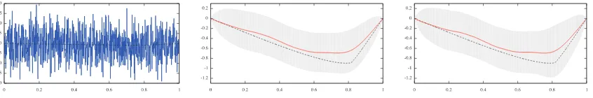
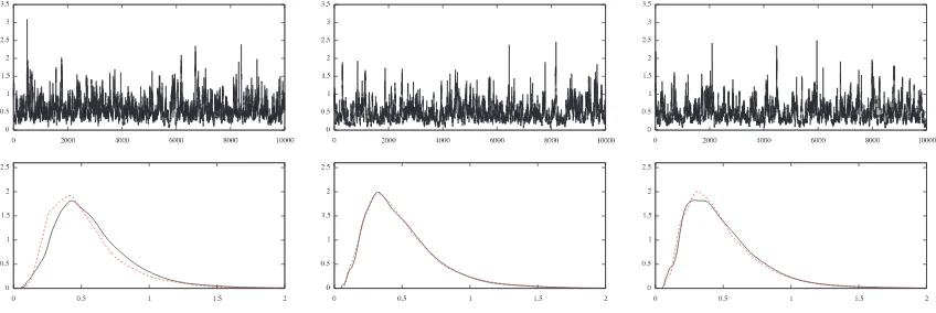
[image:19.612.93.516.563.633.2]In Figure1we plot the true solution, the noisy data, and the sample means and credibility bounds using CA and NCA forN = 8192. The sample means and credibility bounds at other discretization levels of the unknown are similar and are therefore omitted.
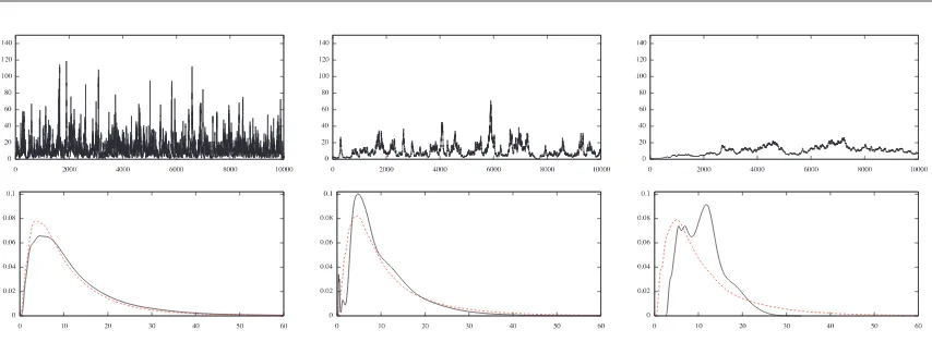
Figure 2. CA: δ-chains (top) and kernel density estimates of the posterior onδ (bottom) for dimensions
N = 32,512, and 8192 left to right. In dashed red in the density plots is the density estimate using MA, considered as the gold standard.
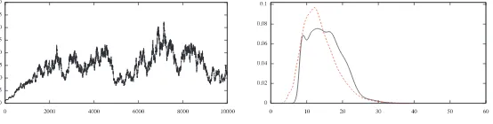
[image:20.612.96.523.427.570.2]In Figure 2 we see that for CA, in small dimensions the δ-chain has a healthy mixing; however, as predicted by Theorem 3.4, as N increases, it becomes increasingly slower and exhibits diffusive behavior. This is also reflected in the density plots where we observe that as N increases, the kernel density estimates computed using CA look less and less like the density estimates computed using MA which we consider to be optimal in this setting. In Figure 3 we see that for NCA, as expected, theδ-chain appears to be robust with respect to the increase in dimension; this is also reflected in the density estimates using NCA which now look very close to the ones obtained using MA for all discretization levels.
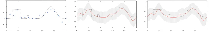
Figure 3. NCA:δ-chains (top) and kernel density estimates of the posterior onδ(bottom) for dimensions
N = 32,512, and 8192 left to right. In dashed red in the density plots is the density estimate using MA, considered as the gold standard.
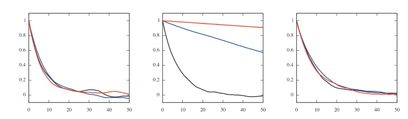
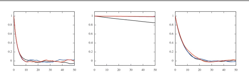
Figure 4. Autocorrelation functions ofδ-chain, dimensions32(black),512(red), and8192 (blue); left for MA, middle for CA, and right for NCA.
5.2. Linear Bayesian inverse problem with coarse data using finite difference discretiza-tion. We consider a modification of the simultaneously diagonalizable setup described in sub-section 4.1, where X =L2(I),I = (0,1), and we allow K to map X into RM and hence have data y ∈ RM. This setting is not directly covered by the theoretical analysis presented in section 3; however, our theory readily generalizes to cover this setting; we refer the interested reader to the Ph.D. thesis [2, section 4.5] for more details. The generalized analysis holds again under Assumptions3.2on the discrete level based on intuition which holds for problems satisfying Assumptions3.1 on the underlying continuum model for the unknownu.
In particular, we consider the problem of recovering a true signalu†by observing a blurred version of it at M equally spaced points{M1+1, . . . ,MM+1}, polluted by additive independent Gaussian noise of constant variance λ−1. We define A0 to be the negative Laplacian with Dirichlet boundary conditions in I. We let P be defined as in subsection 1.2.2 and define
˜
K = (I+ 1001π2A0)−1, and we consider the case K = PK˜, C0 =A−01, and C1 = IM in the setting of subsection 1.1and whereIM is theM×M identity matrix. Notice that due to the
smoothing effect of ˜K, the operatorK is bounded in X. However, due to the presence ofP,
K is not simultaneously diagonalizable withC0.
We now check that this problem satisfies Assumptions3.1. Indeed, assuming without loss of generality that λ = δ = 1, by [39, Example 6.23] we have that the posterior covariance
and mean satisfy (1.5) and (1.6), and hence C−12
0 m(y) = C−
1 2
0 (C−01+K∗K)−1K∗y = (I + C12
0K∗KC
1 2
0)−1C
1 2
0K∗y, where C
1 2
0K∗y ∈ X, and (I+C
1 2
0K∗KC
1 2
0)−1 is bounded in X by the
nonnegativity ofC 1 2
0K∗KC
1 2
0. Furthermore, we have that Tr(C−
1 2
1 KC0K∗C−
1 2
1 ) = Tr(KC0K∗), which is finite since KC0K∗ is anM ×M matrix.
We discretize this setup at level N, using the finite difference approximation as explained in subsection 1.2.2. In particular, we discretize A0,P, and P∗ by replacing them with the matricesA0, P, and (N+1)PT, respectively, as in subsection1.2.2; this induces a discretization of the operators K and C0 by replacing them with the corresponding matrices K and C0 calculated through the appropriate functions of A0 and P. In defining K, we also replace the identity operator by the N×N identity matrix. We do not prove that this discretization scheme satisfies Assumptions 3.2; however, we expect this to be the case.