Low degree multi spectral p mode fitting

(1)

http://wrap.warwick.ac.uk

Original citation:

Howe, R., Broomhall, A. -M., Chaplin, W. J., Elsworth, Y. and Jain, K.. (2013) Low-degree multi-spectralp-mode fitting. Journal of Physics: Conference Series, Volume 440 . Article number 012011. ISSN 1742-6596

Permanent WRAP url:

http://wrap.warwick.ac.uk/59072

Copyright and reuse:

The Warwick Research Archive Portal (WRAP) makes this work of researchers of the University of Warwick available open access under the following conditions.

This article is made available under the Creative Commons Attribution 3.0 (CC BY 3.0) license and may be reused according to the conditions of the license. For more details see: http://creativecommons.org/licenses/by/3.0/

A note on versions:

The version presented in WRAP is the published version, or, version of record, and may be cited as it appears here.

(2)

Download details:

IP Address: 137.205.202.72

This content was downloaded on 23/01/2014 at 15:54

Please note that terms and conditions apply.

View the table of contents for this issue, or go to the journal homepage for more 2013 J. Phys.: Conf. Ser. 440 012011

(3)

Low-degree multi-spectral

p

-mode fitting

R Howe1

, A-M Broomhall1,2,3, W J Chaplin1, Y Elsworth1

and K Jain4 1

School of Physics and Astronomy, University of Birmingham, UK

2

Centre for Fusion, Space and Astrophysics, Department of Physics, University of Warwick, Coventry, CV4 7AL

3

Institute of Advanced Study, University of Warwick, Coventry, CV4 7AL

4

National Solar Observatory, 950 N Cherry Ave., Tucson, AZ 85719, USA E-mail: [email protected]

Abstract. _{We combine unresolved-Sun velocity and intensity observations at multiple}

wavelengths from the Helioseismic and Magnetic Imager and Atmospheric Imaging Array onboard the Solar Dynamics Observatory to investigate the possibility of multi-spectral mode-frequency estimation at low spherical harmonic degree. We test a simple multi-spectral algorithm using a common line width and frequency for each mode and a separate amplitude, background and asymmetry parameter, and compare the results with those from fits to the individual spectra. The preliminary results suggest that this approach may provide a more stable fit than using the observables separately.

1. Introduction

The 1700 and 1600 ˚A bands of the Atmospheric Imaging Assembly (AIA) onboard the Solar Dynamics Observatory (SDO) are formed higher in the solar atmosphere than the lines typically used for Doppler velocity measurements – around 360 km for the 1700 ˚A and 480 km for the 1600 ˚A band [1], extending from the upper photosphere into the chromosphere. They neverthless show a clear p-mode spectrum for integrated-Sun measurements [2]. Although the velocity and intensity spectra formed at different heights differ in many details and reflect different mode physics, the underlying mode frequency and lifetime should be independent of the height of formation or the details of the observation, allowing us to use several spectra together to obtain an improved estimate of the underlying mode parameters. In this article, we attempt to improve our estimates of the parameters of low-degree p-modes, using data from AIA and from the Helioseismic and Magnetic Imager (HMI) also onboard SDO.

2. Data

The data used cover 691 days starting with 13 May 2010, giving a frequency resolution of 17 nHz. Time series were formed from the AIA 1600 ˚A and 1700 ˚A bands and the HMI Doppler Velocity [V], Continuum Intensity [Ic], and Line Core Intensity [Lc, formed by subtracting the Line Depth observable from Ic], using the DATAMEAN keyword supplied with each HMI and AIA image in the JSOC database1

. The heights of formation of the HMI observables are around

1

http:/jsoc.stanford.edu/

Eclipse on the Coral Sea: Cycle 24 Ascending (GONG 2012, LWS/SDO-5, and SOHO 27) IOP Publishing Journal of Physics: Conference Series 440 (2013) 012011 doi:10.1088/1742-6596/440/1/012011

Content from this work may be used under the terms of theCreative Commons Attribution 3.0 licence. Any further distribution of this work must maintain attribution to the author(s) and the title of the work, journal citation and DOI.

(4)

and background parameters were independent for each spectrum. The peak profile was that of [5]:

P(x) =A(1 +Sx) 2

+S2

(1 +x2₎ +B, (1)

where A is the amplitude,S is the asymmetry parameter, B is the background parameter and x = 2(ν −ν0)/γ, γ being the FWHM and ν0 the central frequency. For the sake of a more stable fit we fixed the rotational splitting at 0.41 µHz and also fixed the amplitude ratios of the rotationally split components, but the relative amplitudes of ℓ= 1,3 and ℓ= 0,2 mode pairs were not constrained.

We use an AMOEBA-based [6] maximum likelihood estimation fitting algorithm, with a first pass on a lightly (15-bin) smoothed power spectrum to improve the first guesses for the final fit. We fit each ℓ = 0,2 and ℓ = 1,3 pair separately in a 50-µHz frequency window. For each mode pair, the observables were scaled so that all of the smoothed spectra had the same maximum value and roughly the same weight in the fit. Formal uncertainties on the estimated parameters were approximated using the inverse of a numerically computed Hessian matrix, neglecting off-diagonal terms to save computing time.

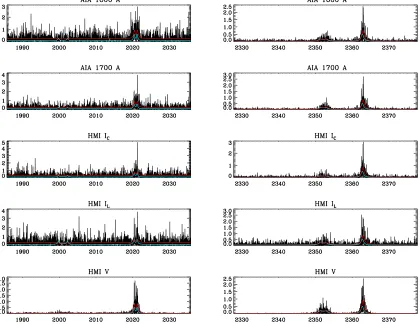
In Figure 1 we show some sample multi-spectral fits with the first-guess and final models superimposed on the spectrum. This figure also serves to illustrate the differing signal-to-noise ratios of the various observables, with HMI Ic having the lowest signal-to-noise and HMI V the highest. After fitting, we rejected results where the fit did not converge properly (non-finite error), as well as those with unreasonably small line widths or negative amplitude parameters. This weeding does not remove all of the obviously “out of line” fits, particularly when signal-to-noise is poor, and some further criteria will be needed in future work. To test the efficacy of the simultaneous fitting, we fitted the five spectra both together and individually using the same model and first-guess parameters.

4. Results and discussion

In Figure 2 we show the linewidth and frequency parameters from the multi-spectral and single-spectral fits, with frequency being represented by the difference between the input first-guess and final estimated frequency so as to show the scatter. By definition all of the frequency and width estimates fall on top of one another for the multi-spectral case, so HMI V dominates the left-hand panels because it was plotted last and has the largest number of successful fits. There are a couple of cases where the multi-spectral fit failed for HMI V but succeeded for HMI Lc, which show as green points. Clearly the scatter in the frequency and width estimates is larger in the single-fit case for the noiser observables, with many of the width estimates falling so far off the curve as to indicate that the fit has effectively failed in these cases.

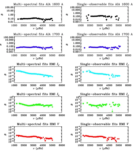
Figures 3, 4 and 5 show the amplitude, background and asymmetry for each observable. For every observable except HMI V (which has much the highest signal-to-noise ratio), the simultaneous fit results in a larger number of successful parameter determinations than the individual fits, where success is defined as having all of the parameters for a given mode and observable pass the simple checks outlined above. The amplitude and background results also seem to follow a smoother curve for the multi-spectral fits, particularly for the weak ℓ = 3

(5)

[image:5.595.97.517.119.449.2]

Figure 1. Sample segments of spectra for the various observables. The light-blue curve shows the first-guess model and the red curve the final fit.

Figure 2. Fitted frequency relative to first-guess frequency (top) and fitted line width (bottom) for the multi-spectral fit (left) and for the individual spectral fits (right). Black represents AIA 1600 A, blue AIA 1700 A, light blue HMI Ic, green HMI Lc, and red HMI V; the different degrees are shown as circles (ℓ= 0), squares (ℓ= 1), diamonds (ℓ= 2) and triangles (ℓ= 3).

[image:5.595.120.481.519.696.2]

(6)

[image:6.595.73.529.112.622.2]

Figure 3. Comparison of fitting results from multi-spectra (left) and single (right) fits showing amplitude for each observable. The different degrees are shown as circles (ℓ= 0), squares (ℓ= 1), diamonds (ℓ= 2) and triangles (ℓ= 3).

(7)

[image:7.595.72.529.107.624.2]

Figure 4. Comparison of fitting results from multi-spectral (left) and single-spectrum (right) fits showing background parameter for each observable. Circles indicate ℓ = 0,2 pairs and squaresℓ= 1,3.

(8)

[image:8.595.82.528.109.622.2]

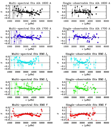
Figure 5. Comparison of fitting results from multi-spectral (left) and single (right) fits, showing asymmetry parameter for each observable. The different degrees are shown as circles (ℓ = 0), squares (ℓ= 1), diamonds (ℓ= 2) and triangles (ℓ= 3).

(9)

modes in the intensity observables. This may be because the information from the HMI V helps to fix the frequency of these modes and ensure that the correct peak is being fitted even when it is buried in the noise. The asymmetry estimates are noisier, but the predominantly negative asymmetry for HMI V, and positive asymmetry for HMI Ic, are clearly seen, whereas the observables formed higher in the atmosphere – the AIA bands and HMI Lc – show a tendency towards positve asymmetry at low frequencies and negative at high frequencies. As the asymmetry depends on the interaction of the modes with the solar background noise, such as granulation, this may perhaps be understood as a lesser influence of granulation higher in the atmosphere. At the highest frequencies, close to the acoustic cut-off, where the modes are broad and not resolved, the fitting is less robust and the trend is less clear, but there are hints that the HMI Ic asymmetry decreases again, while those for the other observables may be increasing.

The results from this preliminary exercise are promising, but there is plenty of room to improve the method. A more sophisticated fitting algorithm might well give better results even for the single-spectrum case. To take full advantage of the multiple observables we need to use the phase and coherence information as well as the power spectra. We hope to do this in future work.

Acknowledgments

HMI data courtesy of SDO (NASA) and the HMI consortium. The National Solar Observatory is operated by the Association of Universities for Research in Astronomy (AURA), Inc. under a cooperative agreement with the National Science Foundation. This work was partly supported by NASA grant NNH12AT11I to NSO. RH acknowledges computing support from NSO.

References

[1] Fossum A and Carlsson M 2005 Astrophys. J.625 556–562

[2] Howe R, Hill F, Komm R, Broomhall A, Chaplin W J and Elsworth Y 2011 Journal of

Physics Conference Series 271 012058–+

[3] Norton A A, Graham J P, Ulrich R K, Schou J, Tomczyk S, Liu Y, Lites B W, L´opez Ariste A, Bush R I, Socas-Navarro H and Scherrer P H 2006 Solar Phys. 239 69–91 (Preprint

arXiv:astro-ph/0608124)

[4] Fleck B, Couvidat S and Straus T 2011 Solar Phys.271 27–40 (Preprint 1104.5166) [5] Nigam R and Kosovichev A G 1998 Astrophys. J. Lett. 505 L51–54

[6] Press W H, Flannery B P and Teukolsky S A 1989 Numerical recipes. The art of scientific

computing (FORTRAN Version) (Cambridge University Press)