Statistical Delay QoS Driven Energy Efficiency and Effective Capacity Tradeoff for Uplink Multi User Multi Carrier Systems

Statistical Delay QoS Driven Energy Efficiency and

Effective Capacity Tradeoff for Uplink Multi-User

Multi-Carrier Systems

Wenjuan Yu, Leila Musavian and Qiang Ni

Abstract—In this paper, the total system effective capacity

(EC) maximization problem for the uplink transmission, in a multi-user multi-carrier OFDMA system, is formulated as a combinatorial integer programming problem, subject to each user’s link-layer energy efficiency (EE) requirement as well as the individual’s average transmission power limit. To solve this challenging problem, we first decouple it into a frequency provisioning problem and an independent multi-carrier link-layer EE-EC tradeoff problem for each user. In order to obtain the subcarrier assignment solution, a low-complexity heuristic algorithm is proposed, which not only offers close-to-optimal solutions, while serving as many users as possible, but also has a complexity linearly relating to the size of the problem. After obtaining the subcarrier assignment matrix, the multi-carrier link-layer EE-EC tradeoff problem for each user is formulated and solved by using Karush-Kuhn-Tucker (KKT) conditions. The per-user optimal power allocation strategy, which is across both frequency and time domains, is then derived. Further, we theoretically investigate the impact of the circuit power and the EE requirement factor on each user’s EE level and optimal average power value. The low-complexity heuristic algorithm is then simulated to compare with the traditional exhaustive algorithm and a fair-exhaustive algorithm. Simulation results confirm our proofs and design intentions, and further show the effects of delay quality-of-service (QoS) exponent, the total number of users and the number of subcarriers on the system tradeoff performance.

Index Terms—Link-layer energy-rate tradeoff, delay-outage

probability, effective capacity, energy efficiency.

I. INTRODUCTION

Green communication networks, which not only emphasize on spectrum efficiency (SE), but also promise high energy efficiency (EE), have become imperative needs of future communication systems. However, by nature, EE and SE could require conflicting design approaches. From the information-theoretic point of view, the EE-SE tradeoff problem in a down-link orthogonal frequency division multiple access (OFDMA) network was analyzed in [2], in which the impact of the channel power gain and the circuit power on the EE-SE relation was discussed. Considering the cognitive radio net-works, a multi-objective optimization was formulated in [3], in which the ergodic capacity was maximized and the total

This work was supported in part by the China Scholarship Council, UK EPSRC under grant number EP/K011693/1, and grant number EP/N032268/1, and the EU FP7 under grant number PIRSES-GA-2013-610524. Part of this work was presented in [1]. (Corresponding author: Qiang Ni)

W. Yu and Q. Ni are with the School of Computing and Communica-tions, InfoLab21, Lancaster University, LA1 4WA, UK (Emails: {w.yu1, q.ni}@lancaster.ac.uk). L. Musavian is with the School of Computer Science and Electronic Engineering, University of Essex, CO4 3SQ, UK (Email: [email protected]).

transmission power of femtocell base stations was minimized. A general power consumption model in multi-user OFDMA systems, including the transmission power, signal processing power, and circuit power from both the transmitter and the receiver sides, was first established in [4]. Then the authors in [4] proposed a joint optimization method to iteratively find the optimal solution for the EE-maximization problem, subject to a peak transmit power constraint and a minimum system data rate requirement. The EE and SE tradeoff problem has also been extensively studied for other kinds of wireless communication networks, such as energy-constrained wire-less multi-hop networks with a single source-destination pair [5], general narrowband interference-limited systems [6] and OFDMA-based cooperative cognitive radio networks [7]. In the aforementioned studies, however, the system throughput was given by Shannon limit, without taking into account delay constraints. For systems with delay-sensitive applica-tions, such as video conferencing and online gaming, the physical-layer based power and rate adaptation techniques may not be efficient. In fact, 5G, the next generation of mobile communication technology, has been anticipated to offer >1 Gbps downlink data rate, sub-1ms end-to-end latency and 90% reduction in network energy usage [8]. This infers that the future wireless communication networks are targeted at satisfying the end-user applications’ delay quality-of-service (QoS) requirements, while at the same time increasing EE and SE for green communications.

considers and confines the delay bound violation probability to a required value range. In this direction, the authors in [13] introduced a link-layer capacity notion supporting statistical delay QoS requirements, which is the concept of effective ca-pacity (EC). Formulated as the dual of the effective bandwidth, EC specifies the maximum arrival rate that can be supported by a wireless channel given that a target delay-outage probability requirement is guaranteed [13] [19]. Therefore, EC can be regarded as the link-layer SE. The link-layer EE, henceforth, can be formulated as the ratio of the EC to the total power expenditure [14].

Due to the inconsistent property of the link-layer EE and EC, many researchers have elaborately studied how to balance the two metrics. Considering frequency flat-fading channels, an optimal power allocation strategy to maximize EC sub-ject to a link-layer EE constraint, for delay-limited mobile multimedia applications was obtained in [15]. For a Rayleigh flat-fading channel under delay-outage probability constraints, a multi-objective optimization problem to jointly maximize EE and EC was formulated and solved in [16]. The above mentioned papers, however, focus on a point-to-point single-channel communication system.

We note that based on the theory of Shannon limit, the total average rate of a multi-carrier system is a linear sum-mation of each subcarrier’s achievable average rate. This, however, does not apply to systems with limited statistical delay requirements. Specifically, in delay-constrained systems, the concavity and monotonicity of the EC do not remain homogeneous for single-carrier and multi-carrier systems [17]. In addition, for systems with statistical delay QoS constraints, it has been proven that the optimal power allocation strategy for single-carrier communications cannot be simply extended to the multi-carrier communications [17]. Hence, considering a single-user multi-carrier link over a frequency-selective fading channel, the delay-constrained EC maximization and EE max-imization problem were separately addressed in [17] and [18], respectively. However, the link-layer EE-EC tradeoff problem for the multi-carrier communications is not investigated and analyzed in the literature. Especially, when we consider a multi-user multi-carrier network, the link-layer EE-EC tradeoff problem becomes more challenging. The formulated problem will be a complex combinatorial integer programming prob-lem, rather than a convex optimization problem in [17] which was solved using Lagrangian method. In [20] and [21], an EE optimization problem with statistical delay provisioning and per-user’s EC requirement constraint was analyzed for a downlink multi-user OFDMA network. In these papers, the power allocation for each subcarrier is assumed to be only related to its subcarrier’s channel power gain, and not related to the same user’s other subcarriers’ channel power gains. Therefore, based on this assumption and the independent and identically distributed (i.i.d.) property of all subcarriers, the EC value for a single-user multi-carrier system can be formulated as a linear summation of the EC values of all subcarriers. While this independent optimization approach is optimal in maximizing the Shannon capacity (e.g., water-filling power control for multi-carrier transmissions), it is not the optimal policy to maximize the EC-based problems for an arbitrary statistical delay provisioning [17]. In this paper, we will not

make this assumption, and aim to derive the optimal power allocation strategy for each user, which is not only across the time domain, but also across the frequency domain.

In this paper, we target to maximize the system total EC for the uplink transmission in a multi-user multi-carrier OFDMA network, subject to each user’s required link-layer EE performance level and its individual resource limits. We decouple the problem into two parts and provide the subcarrier assignment solution and optimal power allocation strategy for each user. In more detail, we propose a low-complexity heuristic algorithm, which first allocates each served user the exact number of its required subcarriers, and then implements the optimal per-user power allocation strategy to calculate each user’s current EC value. Finally, the remaining subcarriers will be allocated by adopting the strategy that the user with current minimum EC value has the allocation priority.

To sum up, this paper has the following contributions:

• A novel total EC maximization problem for the uplink transmission, in a multi-user multi-carrier OFDMA sys-tem, is formulated as a complex combinatorial integer programming problem, subject to each user’s link-layer EE requirement and the individual’s average input power limit. A new adjustable EE requirement factor is defined to further tune each user’s EE constraint value, which transforms the formulated problem into a tradeoff prob-lem between the system total EC and the users’ individual EE achievements.

• The formulated challenging problem is first decoupled into a frequency provisioning problem and an indepen-dent link-layer multi-carrier EE-EC tradeoff problem for each user. The traditional exhaustive algorithm and a fair-exhaustive algorithm are introduced first, followed by a low-complexity heuristic algorithm, which cares about user fairness, offers a close-to-optimal performance, and also has a complexity linearly relating to the size of the problem.

• The independent multi-carrier power-constrained link-layer EE-EC tradeoff problem is then solved and analyzed for each user, given a subcarrier assignment matrix. The optimal power allocation strategy, which is across frequency and time domains, and the Pseudocode of the power allocation process are derived and proposed. • We prove that each user’s average optimal power level

monotonically decreases with its EE requirement factor. Furthermore, we prove that each user’s link-layer EE value monotonically decreases with its circuit power value, but increases with its EE requirement factor. • Simulation results reveal that when there is a link-layer

EE constraint, each user’s operational tradeoff EC value 1 _{will not show a monotonic trend with its delay QoS} exponent. Further, the tradeoff EC value achieved with a smaller number of available subcarriers may be higher than the one obtained with larger number of subcarriers.

Fig. 1: Uplink transmission in a multi-user multi-carrier network.

II. SYSTEMMODEL ANDPROBLEMFORMULATION

A. Multi-user Multi-carrier System Model

We consider the uplink transmission, where the K active users send their own information to the base station, in a multi-user multi-carrier OFDMA system depicted in Fig. 1. A total bandwidth of B is divided into N subcarriers, each

with a bandwidth of B

N. Assume that each subcarrier is

exclusively assigned to at most one user at each time to avoid interference among different users. The total number of allocated subcarriers for all users does not exceed the available frequency resources. Therefore, a feasible subcarrier assignment indicator matrix can be denoted as φ, which satisfies

φ∈Φ,

(

[φk,n]K×N |φk,n ∈ {0,1}, K

X

k=1

φk,n ≤1,

K

X

k=1

N

X

n=1

φk,n≤N, k∈ K0, n∈ N0

)

. (1)

Here, Φ denotes the set of all possible subcarrier alloca-tion indicator matrices, and K0 = {1,2, . . . , K}, N0 =

{1,2, . . . , N} denote the set of all users and all subcarriers, respectively. The number of allocated subcarriers for the kth user is denoted by Nk, namely, Nk =

N

P

n=1

φk,n, and the

bandwidth allocated to the kth _{user is denoted by B} k, i.e.,

Bk=Nk

B N.

Each transmitter implements a first-in-first-out (FIFO) buffer, which prevents loss of packets that could occur when the source rate is higher than the service rate, at the expense of increasing the delay [13]. The upper-layer packets are divided into frames at the data-link layer and are stored at the transmit buffer. The frames are then split into bit streams at the physical layer. By utilizing perfect channel state information (CSI) knowledge fed back from the receiver and the predetermined statistical QoS constraint, adaptive modulation and coding (AMC) and adaptive power control policy are applied at the transmitter side [17]. Then, the bit streams are read out of the buffer and are transmitted through the wireless fading subcarriers. At the receiver side, the reverse operations are performed and the frames are recovered for further processing. We assume that each subcarrier experiences block fading, i.e., the channel gains of N subcarriers are invariant within a

Fig. 2: Queuing system model for each transmitter.

fading-block’s time durationTf, but independently varies from one fading block to another. In addition, the length of each fading-block, Tf, is considered to be an integer multiple of the symbol duration Ts, and is assumed to be less than the fading coherence time [17].

For the kth _{user on the n}th _{subcarrier at the fading-block} index t, the subcarrier power gain is denoted by γk,n[t], k ∈ K0, n∈ N0. Also, each subcarrier is assumed to experience

i.i.d. additive white Gaussian noise (AWGN) with power spectral density η0

2 . Therefore, the instantaneous maximum

achievable rate of the kth _{user on then}th _{subcarrier at thet}th fading-block is given by

Rk,n[t] =

B

NTflog2 1 +Pk,n[t]

γk,n[t]

Pk Lη0 BN

!

(bits), (2)

where Pk

L denotes the distance-based path-loss power and

Pk,n[t] is the nonnegative transmission power for the kth user on the nth _{subcarrier, at the t}th _{fading-block, i.e.,}

Pk,n[t] ≥ 0. Specifically, for the kth user, the sub-carrier power allocation vector is denoted as Pk[t] =

Pk,1[t] Pk,2[t] ... Pk,N[t]

₂

. The total achievable rate over all allocated subcarriers for thekth_{user, which depends on} the subcarrier allocation indicator matrixφand the subcarrier power allocation vector_P Pk, can be denoted asRk(φ,Pk) = n∈Nk

φk,nRk,n, where Nk is the set of subcarriers allocated

to thekth _user.

B. Multi-user Multi-carrier Effective Capacity and Link-layer Energy Efficiency

For each transmitter, the FIFO buffer is assumed to be a dynamic queueing system with stationary ergodic arrival and service processes, depicted in Fig. 2 [22]. By using the large deviation theory, the queue length processQ(t)converges in distribution to a steady-state queue length Q(∞) such that [22]

− lim

x→∞

ln (Pr{Q(∞)> x})

x =θ, (3)

wherePr{a > b}shows the probability thata > bholds. This definition implies that the probability of the queue length ex-ceeding a certain thresholdxdecays exponentially fast asx in-creases [23]. Note that in (3), the parameterθ(θ >0)indicates the exponential decay rate of the QoS violation probability. A smaller value of θ denotes a looser QoS requirement, while larger θ implies a lower probability of violating the queue length and a more stringent delay constraint. Particularly, when

2_{Since the service rate process of the} kth _{user on the}nth _{subcarrier is}

considered to be stationary and ergodic [17], hereafter, the block index t

θ→0, which refers to a system with no delay constraint, the optimum power allocation strategy is the traditional water-filling approach and the maximum achievable rate is ergodic capacity. For a transmitter withθ→ ∞, the optimum power allocation is the channel inversion with fixed rate transmission technique, under which the delay-limited capacity can be achieved. In other words, the ergodic capacity and the delay-limited capacity can be considered as two extreme cases of the effective capacity.

Taking the delay experienced by a source packet arriving at timet, defined by D(t), into consideration, the probability that the delay exceeds a maximum delay boundDmax, can be estimated as [13]

Pout

delay= Pr{D(t)> Dmax} ≈Pr{Q(t)>0}e

−θµDmax_{, (4)}

where Pout

delay presents the delay-outage probability, Dmax is in the unit of a symbol period, Pr{Q(t) > 0} denotes the probability of a non-empty buffer at time t, and can be approximated by the ratio of the constant arrival rate to the average service rate [17], [22], i.e.,Pr{Q(t)>0} ≈ µ

E[R[t]].

Hence, in order to meet a target delay-outage probability limit

Pout

delay, a source needs to limit its data rate to the maximum of

µ, whereµis the solution to (4).

Assume that the Gartner-Ellis theorem [24, Pages 34-36] is satisfied. For thekth _{user, the EC value, in b/s/Hz, over a} multi-carrier transmission with a total bandwidthBk can be expressed as [13]

Eck(θk,φ,Pk) =−

1

θkTfBk

lnE

h

e−θkRk(φ,Pk)

i

, (5)

whereθk stands for the delay QoS exponent of the kth user which is associated with the statistical delay QoS requirement andE[·]indicates the expectation operator. Henceforth, EC of thekth _{user becomes a function of θ}

k,φ, andPk.

By expanding R_{k(φ,Pk) and inserting it into (5), EC of} thekth _{user can be further expressed as}

Ek

c (θk,φ,Pk) =−

1

θkTfBk

ln

E

e

−θk P n∈N_k

φk,nRk,n

.

(6)

For the multi-user OFDMA network, the overall EC value can be expressed as

Ec(θ,φ,P) =

PK

k=1NkEck(θk,φ,Pk)

PK k=1Nk

(b/s/Hz), (7)

where θ = θ1 θ2 ... θK is the K × 1 vector of delay exponents for all K users. P denotes the transmission power allocation matrix, for all users over all subcarriers, i.e., P ∈ P ,

n

[Pk,n]_K×N ∈R+|Eγk

hPN

n=1φk,nPk,n

i

≤Pk

max, k∈ K0

o

. Here, P is all the possible power allocation matrices, Eγk[·] indicates the expectation over the PDF of γk,

where γk is the kth user’s subcarrier power gains, i.e., γk =

γk,1 γk,2 ... γk,Nk

.Pk

maxrepresents the maximum average power limit of thekth _user.

Moreover, for thekth_{user, we define the link-layer EE as the} ratio of EC to the sum of its circuit powerPk

c, and the average

transmission power scaled by the power amplifier efficiency

ǫ, yielding

EEk_(θ

k,φ,Pk) =

Ek

c(θk,φ,Pk)

Pk

c +

1

ǫEγk

" P

n∈Nk

φk,nPk,n

#. (8)

C. Problem Formulation

From a system point of view, the overall EC value needs to be maximized to achieve the best system performance. On the other hand, from the individual user point of view, each user has its own link-layer EE requirement, average transmission power limit and delay QoS constraint. Therefore, considering a multi-user multi-carrier network, the overall system throughput maximization problem, subject to each user’s resource constraints, can be formulated as

Q1 : max

φ∈Φ,P∈P Ec(θ,φ,P) (9a) subject to: EEk_(θ

k,φ,Pk)≥ηkreq, ∀k, (9b) Eγk

" _N X

n=1

φk,nPk,n

#

≤Pk

max, ∀k, (9c) K

X

k=1

φk,n≤1, ∀n, (9d)

K

X

k=1

N

X

n=1

φk,n≤N, (9e)

φk,n ∈ {0,1}, ∀k,∀n, (9f)

Pk,n≥0, ∀k,∀n, (9g)

whereηk

reqis thekthuser’s required link-layer EE level, defined by a certain ratio of its maximum achievable link-layer EE value, i.e., ηk

req = χkEE×η k,N

max. Here, ηmaxk,N = EEk

Nk=N

Pk=Pk

∗

EE

denotes the kth _{user’s maximum achievable EE value, when} all N subcarriers in the system are allocated to it. Pk∗

EE is the operational average input power which achieves ηk,Nmax. Further, χk

EE ∈[0,1]is an adjustable EE requirement factor, which reveals the strictness of thekth _{user’s required EE level} and directly influences the system performance. In particular,

χk

EE = 0 indicates that the kth user has no EE requirement, while χk

EE = 1means that userk requires an operational EE value at ηk,Nmax. Since ηk,Nmax depends on the individual user’s delay QoS exponent and its maximum averge power limit, its value is different for each user. Therefore, the kth _user’s required EE level ηk

req is different from the other users, even when they have the same EE requirement factors.

Due to the conflicting property of the total system EC and each user’s personal EE achievement, after introducing χk

III. OPTIMAL ANDSUB-OPTIMALSOLUTIONS

Since we assume that one subcarrier can be assigned to only one user at a time, therefore there could beKN _possible subcarrier assignments [25]. Hence, the complexity of the above combinatorial integer programming problem in finding the jointly optimal subcarrier and power allocation grows exponentially with the number of subcarriers. Furthermore, we note that it is very difficult to jointly obtain the optimal subcarrier allocation sets and all power allocation values in every frame, due to the reasons below. Firstly, from (6), we can notice that the EC formulation of the kth _{user not only} requires the multiplication of two unknown parameters, i.e.,

φk,n, and Rk,n, but also involves the expectation over the joint PDF of all subcarriers’ channel power gains, i.e., γk. Secondly, the expectation and the multiplication operations cannot be interchanged, even if all subcarriers are assumed to be i.i.d., and that is because the power allocation value on each subcarrier is related to the other subcarriers.

Henceforth, in order to make the formulated problem Q1

tractable, we divide the solving process into two steps: fre-quency provisioning which decides the number of subcarriers to be allocated to each user; and then optimal power allocation for each user over all its allocated subcarriers. Specifically, the proposed frequency provisioning algorithms, which are independent of the instantaneous CSI knowledge in each frame, will be implemented only once within a period of time. On the other hand, for each user, the proposed optimal power allocation strategy on each subcarrier, not only relies on the instantaneous CSI of this subcarrier, but also depends on the other subcarriers’ CSI knowledge in each frame.

We start from introducing three frequency provisioning algorithms: traditional exhaustive algorithm, fair-exhaustive al-gorithm and our proposed low-complexity heuristic frequency allocation algorithm. After obtaining the subcarrier assign-ments, the optimal power allocation strategy for each single-user multi-carrier system will then be derived and obtained in Section III-B.

A. Frequency Provisioning Algorithms

By applying frequency provisioning, we assume that all subcarriers follows the same distribution. It is the number of designated subcarriers which matters, regardless where those subcarriers are located in the frequency band [25]. To reduce the problem complexity and the solving time, we first build a pre-calculated offline database D which stores all users’ maximum achievable link-layer EE values, i.e., ηmax=η1

max ηmax2 ... ηmaxK

T

, in terms of certain settings of Pc, θ and N. Here ηkmax is a 1 ×N vector of the k

th user’s maximum achievable EE values with different number of allocated subcarriers, i.e.,ηk

max=

ηmaxk,1 ηk,max2 ... ηmaxk,N

.

Defineηreq=η1

req ηreq2 ... ηreqK

T

as theK×1 vector of the EE requirement values for allKusers, then we will trans-formηreqto aK×1vector which specifies all users’ required number of subcarriers, i.e., Sreq = S1

req Sreq2 ... SreqK

T . Let us consider thekth _{user as an example. Its required} link-layer EE value is denoted by ηk

req, and correspondingly, its subcarrier requirement value will be stored asSk

req.

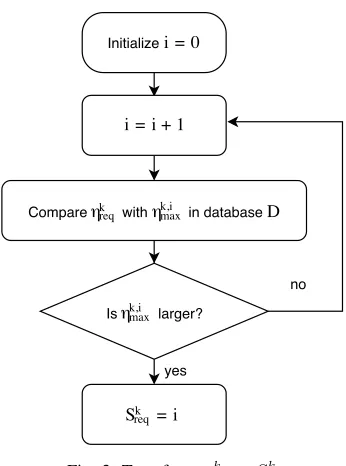
Fig. 3: Transformηk

reqtoS

k

req.

To obtainSk

req, we provide a flowchart in Fig. 3 to compare

ηk

req withηkmax. If the maximum achievable EE value obtained with i subcarriers is larger than the required EE value, i.e.,

ηmaxk,i ≥ηkreq, then we can conclude that the minimum number of subcarriers required to satisfy thekth_{user’s EE requirement}

ηk

req, isi, i.e., Sreqk =i. Henceforth, allK users’ EE require-ments inηreqcan be transformed to the subcarrier requirement vectorSreq, by utilizing the flowchart in Fig. 3. In this way, the feasibility of each user’s EE constraint can be easily checked by comparing the number of allocated subcarriers with the number of required subcarriers.

1) Traditional Exhaustive Algorithm

The traditional way to solve an NP-hard problem, like the one we formulated in (9a)-(9g), is to carry out an exhaustive search, which systematically enumerates all possible combi-nations and finally locates the solution which optimizes the objective function and satisfies all the problem constraints [25]. Specifically, for problem Q1, the set of feasible com-binations is found first. Then, the optimal power allocation strategy proposed in the next section, will be applied to all the feasible combinations. Finally, the feasible combination which offers the maximum system throughput will be chosen as the optimal solution. Although exhaustive search is able to find the optimal frequency provisioning solution, it also lacks user fairness and has a high computational complexity which exponentially grows with the size of the problem.

2) Fair-Exhaustive Algorithm

most. Secondly, the set of feasible subcarrier allocation vectors is found, in which each allocation vector not only satisfies all served users’ subcarrier requirements, but also serves the maximum allowed number of users. Then, the optimal power allocation strategy proposed in Section III-B will be applied to all feasible allocation vectors to locate the fair and optimal solution which outperforms the others.

Clearly, by enumerating all possible subcarrier allocation vectors which can serve the allowed maximum number of users, the above proposed algorithm exhaustively find the optimal solution in a fair way. Although the fair-exhaustive algorithm is less complex compared to the traditional exhaus-tive algorithm, but its computational complexity is still very high, especially when the number of available subcarriersN

is large. To further reduce algorithm complexity, we provide the following heuristic algorithm, which is simple, fair and close-to-optimal.

3) Heuristic Algorithm

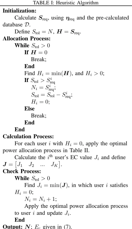
There are three steps included in the proposed heuristic frequency provisioning algorithm, which are allocation pro-cess, calculation process and check process. Firstly, in order to serve as many users as possible, in the allocation process, we start from the user which requires the minimum number of subcarriers. Each served user will be allocated the exact number of its required subcarriers, so that all the allocated users can satisfy their EE requirements. The allocation will be repeated until the remaining subcarriers run out, or there are not enough subcarriers to satisfy the next user’s EE requirement, or all users’ subcarrier requirements have already been satisfied. Then, the calculation process starts, in which each served user operates the optimal power allocation strategy described in Table II to obtain its corresponding EC value. In the check process, we aim to maximize the system throughput, based on the strategy that the user with current minimum EC value has the allocation priority. Therefore, the remaining subcarriers will be assigned one-by-one to the user who has the current minimum EC value, until all subcarriers run out.

Assume the final subcarrier allocation vector is denoted by N =N1 N2 ... NK

. The Pseudocode of the proposed heuristic algorithm is illustrated in Table I. We note that, the proposed algorithm only needs at most K−1 comparisons per iteration, given that each user’s EC values with various number of subcarriers, is pre-calculated off-line and is stored in a database. Therefore, the heuristic algorithm offers a relatively low computational complexity comparing to the two exhaustive algorithms whose complexity exponentially increase with the number of subcarriers. On the other hand, later, in simulation results, we will demonstrate that the proposed low-complexity algorithm offers a close performance with the fair-exhaustive algorithm.

Now, let us analyze and explain the strategies utilized in the proposed heuristic algorithm. Firstly, in the allocation process, the heuristic algorithm starts the allocation from the user which has the minimum subcarrier requirement. Assume that useri

has the relatively small number of required subcarriers,Si req. By regarding θi and χiEE as the two influencing parameters onSi

req, a small value of Sreqi may result from the following two possibilities: 1) user i has a small delay QoS exponent

TABLE I: Heuristic Algorithm

Initialization:

CalculateSreq, usingηreq and the pre-calculated databaseD.

DefineStol=N,H=Sreq.

Allocation Process: WhileStol>0

IfH= 0

Break;

End

Find Hi= min(H), andHi>0;

IfStol> Sreqi

Ni=Sreqi ;

Stol=Stol−Sireq;

Hi= 0;

Else

Break;

End End

Calculation Process:

For each useri withHi= 0, apply the optimal power allocation process in Table II.

Calculate theith _{user’s EC valueJ}

i and define J =J1 J2 ... JK

.

Check Process: WhileStol>0

Find Ji= min(J), in which useri satisfies

Hi= 0;

Ni=Ni+ 1;

Apply the optimal power allocation process to useriand updateJi.

End

Output:N;Ec given in (7).

θi and the same χiEE value, comparing to the other users; 2) userihas a small EE requirement factorχi

EE, and the sameθi value, comparing to the others. For the first situation, a small delay QoS exponent θi means a loose requirement on delay QoS, which will offer a bigger EC value, when the allocated number of subcarriers and χi

EE are fixed. Meanwhile, for the second situation, a small value ofχi

EEalso provides a larger EC value, because now the EE requirement constraint is easy to be satisfied and the multi-carrier system will have more resource and flexibility to maximize the EC performance. Consequently, the design idea of the allocation process not only makes sure that as many users as possible can be served, but also intends to serve the user which can contribute a larger EC value.

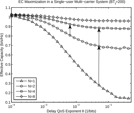
10−4 10−3 10−2 10−1 0.1 0.2 0.3 0.4 0.5 0.6 0.7 0.8 0.9 1 1.1

Delay QoS Exponent θ (1/bits)

Effective Capacity (b/s/Hz)

EC Maximization in a Single−user Multi−carrier System (BT_f=200)

N=1 N=2 N=4 N=8

Fig. 4: Effective capacity versus delay QoS exponentθ, for various values ofN.

number of subcarriers, when we allocate each user two more subcarriers, the user with relatively smaller EC value, namely, the one which has larger delay QoS exponent, will provide a larger EC-increase. Simulation results in Section IV confirm the effectiveness of our design method, and inform that the proposed heuristic algorithm offers very close performance with the fair-exhaustive algorithm.

B. Optimal Power Allocation For A Single-user Multi-carrier System

Given a subcarrier assignment matrix φ, the multi-user OFDMA system can be viewed as a frequency-division mul-tiple access (FDMA) system, where each user transmits data through a number of assigned subcarriers independently [26]. Therefore, the original total EC maximization problem, subject to each user’s link-layer EE requirement and maximum aver-age power limit, can be transformed into a link-layer EE-EC tradeoff problem for each single-user multi-carrier system.

Specifically, for thekth _{user, the problem can be expressed} as

Q2 : max

Pk,n≥0

n∈Nk

Eck(θk,Pk) (10a)

s.t. EEk_(θ

k,Pk)≥ηreqk , (10b) Eγk

"_Nk X

n=1 Pk,n

#

≤Pk

max. (10c) By recalling that the total bandwidth allocated to the kth user isBk, the total instantaneous service rate of thekth user is given by

Rk=

Bk Nk Tf Nk X n=1 log2    1+Pk,n

γk,n Pk Lη0 Bk Nk   

 (bits). (11)

By inserting (11) into (5), we get the mathematical expression of EC for thekth_{user. Correspondingly, the link-layer EE for} thekth_{user, as the ratio of EC to the total power expenditure,}

can be obtained. Therefore, problemQ2can be expanded as

Q3 : max

Pr k,n≥0

n∈Nk

−1

αk

log2

 Eγk

 

Nk

Y

n=1

1+NkPk,nr γk,n

−αk

Nk     (12a) s.t. −1 αk log2  Eγk

 QNk

n=1

1+NkPk,nr γk,n

−αk

Nk     Kk ℓ Pk

cr+

1

ǫEγk

_Nk P

n=1 Pr

k,n

≥ηk req,

(12b)

Kk ℓEγk

"_Nk X

n=1 Pr

k,n

#

≤Pk

max, (12c)

where αk ≡

θkTfBk

ln (2) , P

r k,n =

Pk,n

Kk ℓ

, and Pk

cr =

Pk c Kk ℓ . Here Kk

ℓ =PLkη0Bk, which denotes the path loss factor, including both AWGN power and path loss power. Set ηˆk

req =Kℓkηkreq, and Pˆk

max = Pmaxk /Kℓk. Then, Kℓk in (12a)-(12c) can be canceled to scale the system performance with respect to the path loss factor.

From (12a)-(12c), one can notice that the EC expression in a single-user multi-carrier system is not a linear summation of each subcarrier’s achievable EC value. Hence, the concavity and monotonicity of the EC function in a single-subcarrier system cannot be simply extended to the multi-carrier system. In order to find the joint energy and spectral efficient power allocation strategy in a single-user multi-carrier system, we start from analyzing the proposed problemQ3.

By referring to the scaled multi-carrier transmit power vector as Pr

k =

Pr

k,1 Pk,r2 ... Pk,Nr

, we note that the objective function (12a) is concave in Pr

k [18]. Then, the link-layer EE, as the ratio of a concave function over a non-negative affine function in Pr

k, is a quasi-concave function in subcarrier power allocations [18]. Therefore, its upper contour set defined by (12b) is convex [27]. Hence, (12a)-(12c) is a concave optimization problem and the Karush-Kuhn-Tucker (KKT) conditions are both sufficient and necessary for the global optimum value. Specifically, the proposed optimal power allocation strategy for thekth_{user is related to the joint} probability density function (PDF) of the subcarrier power gainsγk, given byρ(γk).

To solve the concave optimization problem (12a)-(12c), we start from analyzing the power-unconstrained problem (12a)-(12b), which paves the way for the power-constrained optimization problem. By transforming (12b) to

− 1

αk

log2

 Eγk

 

Nk

Y

n=1

1 +NkPk,nr γk,n

−αk

Nk

 

 

−ηˆk

req Pckr+

1

ǫEγk

"_Nk X

n=1 Pr

k,n

#!

we get the Lagrangian function as follows

L(P_kr, λ) =−1

αk

log2

 Eγk

 

Nk

Y

n=1

1+NkPk,nr γk,n

−αk

Nk     +λ  − 1

αk

log2

 Eγk

 

Nk

Y

n=1

1 +NkPk,nr γk,n

−αk

Nk

 

 

−ηˆk

req Pckr+

1

ǫEγk

"_Nk X n=1 Pr k,n #!! − N X n=1

µnPk,nr , (14) where λ ∈ R is the Lagrange multiplier associated to (13) andµn is the Lagrange multiplier associated to the constraint

Pr

k,n ≥0,∀n∈ Nk.

At the optimal power allocation, we have

∂L(Pr k, λ)

∂Pr k

= 0. (15)

Because of the complementary slackness condition [27], if

Pr

k,n > 0, then µn = 0, ∀ n ∈ Nk. On the other hand, if

Pr

k,n = 0, ∃ n ∈ Nk, then µn 6= 0. Thus, the following two cases need to be considered to find the optimal power allocation strategy.

1) Case 1:Pr

k,n >0,∀n∈ Nk

In this case, all Nk subcarriers are allocated non-zero transmission power. Therefore, based on the complementary slackness, {µn}Nn=1k = 0. Then, the KKT condition (15) can

be simplified as

Nk

Y

i=1

1 +NkPk,ir γk,i

−αk

Nk ₌ β

γk,n

1 +NkPk,nr γk,n

,

∀ n∈ Nk, (16)

whereβ= ληˆ

k req

ǫ(λ+ 1) log2e

Eγk

 QNk

n=1

1+NkPk,nr γk,n

−αk

Nk

 . By multiplying the right and left-hand sides of the Nk equations in (16), the optimal power allocation strategy can be obtained as

Pk,nr =

1

Nk



 1

βαk1+1QNk

i=1γ

αk

(αk+1)Nk

k,i

− 1

γk,n



,∀ n∈ Nk. (17)

The derived power allocation strategy (17) is optimal only when all subcarriers are assigned with positive powers. If there are one or more subcarriers which are allocated non-positive powers, then the second case needs to be taken into consideration.

2) Case 2:Pr

k,j = 0,∃ j∈ Nk If there exists Pr

k,j ≤0, then the set of subcarriers, which only positive powers should be assigned, needs to be found.

Firstly, we define Nbk as

b

Nk=

  n∈ Nk

1 Nk   1

βαk1+1QNk

i=1γ

αk

(αk+1)Nk

k,i

− 1

γk,n

 ≥0

  .

According to Lemma 1 in [17], the total power must be assigned to the subcarriers which belong to Nbk, while the

subcarriers n 6∈ Nbk should not be allocated any power. Therefore, a new power-unconstrained optimization problem could be expressed as

Q4 : max

Pr k,n≥0

n∈Nbk

−1

αk

log2

 Eγk

  b Nk Y n=1

1+NkPk,nr γk,n

−αk

Nk     (18a) s.t. −1 αk log2  Eγk

 QNbk

n=1

1+NkPk,nr γk,n

−αk

Nk     Kk ℓ Pckr+

1

ǫEγk

" b Nk P n=1 Pr k,n

#! ≥ηk req,

(18b)

whereNbk=|Nbk|represents the cardinality ofNbk. Therefore, if Pr

k,n > 0, ∀ n ∈ Nbk, then, the optimization problem can be solved exactly like Case 1. Otherwise, if there are subcarriersn ∈ Nbk having Pk,nr = 0, then Nbk must be further partitioned by recursively repeating the above process until a set N∗

k can be found, in which all subcarriers are allocated positive powers [18].

After obtaining N∗

k, the optimal power allocations are computed as Pr k,n=          1 Nk    1 β Nk Nk+_αkN∗

k Q

i∈N∗

kγ αk Nk+αkNk∗

k,i

− 1

γk,n

 

, n∈ N∗ k

0, otherwise

(19)

whereN∗

k =| Nk∗|.

The optimal value for β, referred to as β∗_{, is found when} thekth _{user’s EE constraint is satisfied with equality, yielding}

− 1

αk

log2

 Eγk

 

Nk

Y

n=1

1 +NkPk,nr γk,n

−αk

Nk

 

 

−ηˆk

req Pckr+

1

ǫEγk

"_Nk X

n=1 Pr

k,n

#!

= 0. (20)

Note that since EE versus EC is a bell shape curve, the required EE level, if possible, can be achieved at two different EC values, which means that there will be two solutions forβ, i.e.,

β1 andβ2, to satisfy (20). Assume thatPk1=Pk|β=β1, and

Pk2 =Pk |β=β2, where Pk stands for K k ℓEγk

hPNk

n=1P

r k,n

i

. Therefore, the feasible set of the average input power level sat-isfying the EE constraint (12b) can be written asPk1, Pk2

₃

. Considering our intention to maximize EC and the fact that EC is a monotonically increasing function in Pk [18], the optimal average input power value P∗

k, which solves the power-unconstrained problem (12a)-(12b), is chosen as the larger one which satisfies (20), i.e., P∗

k = max

Pk1, Pk2

. Based on the assumption thatPk2is larger thanPk1, therefore P∗

k =Pk2, and correspondingly,β∗=β2. Here we complete

the solving process of the optimal power allocation for the

TABLE II: Optimal Power Allocation Process

Input: φ, θk, Tf, B, N, Nk, Pck, ǫ, Kℓk,γk, Pmaxk , ηkreq

Step 1:

Have a initial guess ofβ.

Repeat

Create (20), using (17) or (19), which applies Monte Carlo method.

Updateβ using bisection method.

Until findβ∗ _{which solves (20).} Calculate Pr

k,n,n∈ Nk.

Calculate P∗

k =KℓkEγk

hPNk

n=1Pk,nr

i

β=β∗

.

Step 2:

IfPk

max< Pk∗: CreateP∗

k=Pmaxk and updateβ∗, correspondingly. CalculatePr

k,n,n∈ Nk, in (17) or (19).

Step 3:

Calculate the value ofEk

c given in (6) and the link-layer EEk value in (8).

Output: hPr k,n, P

∗

k, Eck,EEk

i

power-unconstrained problem (12a)-(12b).

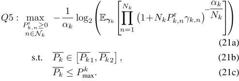
By utilizing the above proposed optimal power allocation strategy, we start to analyze the optimization problem (12a)-(12c) with the average input power constraint. After the feasi-ble set of the average power value for the EE constraint (12b) is found, the power-constrained EC maximization problem for the kth _{user, subject to a link-layer EE constraint, can be} simplified to

Q5 : max

Pr k,n≥0

n∈Nk

− 1

αk

log2

 Eγk

 

Nk

Y

n=1

1+NkPk,nr γk,n

−αk

Nk

   

(21a)

s.t. Pk ∈

Pk1, Pk2

, (21b)

Pk ≤Pmaxk . (21c)

We note that EC is a monotonically increasing function in

Pk [18], therefore, the optimal average power value which solves the problem in (21a)-(21c) will be achieved at one of the three endpoint values, i.e.,Pk1,Pk2, orPmaxk . In more detail, if

Pk2 ≤Pmaxk , the optimal power level Pk∗, equals toPk2, and

the optimal power allocation strategy (17) will be achieved and operated. On the other hand, ifPk1 < Pmaxk < Pk2, the

system has to operate atPk

maxand the optimal power allocation to solve (12a)-(12b) is according to (17), wherein, optimalβ∗

is found such thatP∗

k |β=β∗=Pmaxk . Moreover, ifPmaxk < Pk1,

the power-constrained problem Q5 has no feasible solution. For simplicity, we assume that each user’s maximum available power is always sufficient to support the feasibility of its required EE value, i.e,Pk

max ≥Pk1. Otherwise, the proposed

problem will be infeasible.

To summarize, the Pseudocode of the optimal power alloca-tion process to solve the power-constrained link-layer EE-EC tradeoff problem for thekth_{user, through multiple subcarriers,} is illustrated in Table II. After we obtain the optimal power allocation strategy and optimal operational average power

for problem Q3, further analysis is needed to thoroughly understand and investigate the impact of thekth_{user’s circuit} power value and the EE requirement factor on its link-layer EE-EC tradeoff performance. Hence, we provide the following lemmas4.

C. The effects ofPk

c andχkEEon thekthuser’s EE-EC tradeoff

performance

Lemma 1: The kth _{user’s tradeoff link-layer EE value}

EE P∗ k

decreases with Pk

c.

Proof: The proof is provided in Appendix A.

Furthermore, the tradeoff optimal power value and the system performance can also be influenced by the introduced EE requirement factor. Specifically, when χk

EE increases, the required link-layer EE level increases. Therefore, the final operational link-layer EE value which satisfies the EE require-ment equality increases. Since the proposed tradeoff average power operates at the EE-EC conflicting region, therefore the corresponding EC value will decrease due to the increase in EE level. Hence, we can obtain the following lemma 2.

Lemma 2: The optimal average power valueP∗

k monotoni-cally decreases withχk

EE, but the corresponding link-layer EE value EE P∗

k

increases withχk EE.

Proof: The proof follows the above explanations and is

omitted here due to page limit.

IV. SIMULATIONRESULTS

In this section, we simulate the uplink transmission in a multi-user multi-subcarrier system, in which the fading statistics of the different subcarriers are considered to be i.i.d. Rayleigh distributed such that the subcarrier power gains are realized as exponential random variables with unit mean. We numerically evaluate and compare the performance of the exhaustive algorithm, the fair-exhaustive algorithm, the heuristic algorithm and the algorithm proposed in [25], on the total system EC-maximization problem, under the con-straints of each user’s link-layer EE requirement and average transmission power limit. To further analyze the problem and confirm the lemmas proved in Section III-B, the impact of the delay QoS exponentθ, the EE requirement factorχEEand the circuit-to-noise power ratioPcr on each user’s operational EC value and the total system EC performance is simulated and analyzed. In the following simulations, we assume that

B·Tf = 200, the power amplifier efficiencyǫ= 1, each user’s individual average transmission power limit Pmax = 10dB, unless otherwise indicated.

In order to show the performance of the proposed heuristic algorithm, Fig. 5 shows the results of the total system EC ver-sus the number of subcarriersN, for the heuristic algorithm, the exhaustive algorithm and the fair-exhaustive algorithm. To get Fig. 5, the number of users K is fixed, i.e., K = 4, in which all users have the same settings of EE requirement factor, i.e.,χEE= 0.7, and the circuit-to-noise power ratio, i.e.,

Pcr =−10dB. The delay QoS exponent vectorθ is given by

4_{In these lemmas, we omit the influence of}Pk

max, by assuming that it is large enough to support the optimal power allocation strategy, i.e.,Pk

4 6 8 10 12 14 0.5

0.6 0.7 0.8 0.9 1 1.1 1.2 1.3 1.4 1.5

The number of subcarriers N

Total effective capacity (b/s/Hz)

Heuristic algorithm Fair−exhaustive algorithm Exhaustive algorithm

Fig. 5: The total effective capacity versus the number of subcarriers

N, for heuristic algorithm, exhaustive algorithm and fair-exhaustive algorithm.

4 6 8 10 12 14

0 1 2 3 4 5

The number of subcarriers N

The number of served users

Heuristic algorithm Exhaustive algorithm Fair−exhaustive algorithm

Fig. 6: The number of served users versus the number of subcarriersN, for heuristic algorithm, exhaustive algorithm and

fair-exhaustive algorithm.

[0.001,0.001,0.01,0.01]. For the exhaustive algorithm, when the number of subcarriers N increases, the total system EC value does not change very much, due to the loose delay QoS requirements for all the users. For fair-exhaustive algorithm and heuristic algorithm, the total EC performance curves are very close. This indicates that the proposed heuristic algorithm not only has a low complexity and guarantees user fairness, but also offers close-to-optimal performance.

To further compare the three algorithms, the plots for the number of served users versus the number of subcarriersN are included in Fig. 6. Although the exhaustive algorithm offers the best system performance in Fig. 5, Fig. 6 indicates that it serves the least number of users among all three algorithms. Especially, for the exhaustive algorithm, when N ∈ [4,8], it allocates all subcarriers to only one user, which shows a lack of fairness. On the contrary, for the heuristic algorithm and the fair-exhaustive algorithm, the number of served users shows an increasing trend until it equals to the total number of users K, i.e.,4. This happens because the increase ofN

10−4 10−3 10−2 10−1 100 12

14 16 18 20 22 24 26

Delay QoS exponent θ_k (1/bit)

Average power value (Watt)

N_k=2 N

k=4

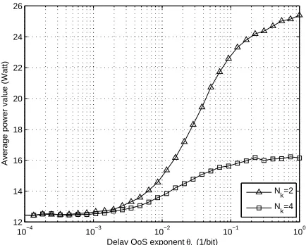
Fig. 7: Average tradeoff optimal power value versus delay QoS exponentθk, for various values ofNk.

means more available frequency resources and the ability of supporting more users increases. We further note that normally, the traditional exhaustive algorithm prefers to choose the best user and allocates all subcarriers to it. However, Fig. 6 indicates that whenN increases from 8 to 14, the number of served users for the exhaustive algorithm increases from 1 to 3 and then stays stable. This means that we may not have one single best user, when all users’ delay QoS exponent values are different.

To understand the above phenomenon thoroughly, we con-sider the kth _{user’s multi-carrier system, and plot Fig. 7 and} Fig. 8 which respectively include the curves of the average power versusθk, and the tradeoff EC value versusθk, for two different values of Nk, with χkEE = 0.2, and Pckr = −10dB. From Fig. 7, we note that with a fixedNk, whenθk increases, the average power value increases. To explain this, we first recall that, thekth _{user’s EE requirement value is defined as a} multiplication ofχk

EEandη k,Nk

max , in whichηmaxk,Nk is a function of θk and Nk. With the fixed values ofNk and χkEE, η

k,Nk

max decreases withθk [18], and in turn, the EE requirement value decreases. Furthermore, the curve of link-layer EE versus aver-age power becomes wider when the user’s delay QoS exponent becomes more stringent [15]. Therefore, when θk increases, the optimal tradeoff average power obtained at a reduced EE requirement equality will become larger. Furthermore, Fig. 7 indicates that with a fixed value of θk, when Nk becomes larger, the average power value reduces. This is due to the fact that when the values ofθk andχkEE are fixed,η

k,Nk

max increases withNk [18], as well as the required EE level. From Fig. 1 in [15], we note that a larger EE requirement will be satisfied at a smaller average power value. Hence, more available number of subcarriers could lead to less average power consumption.

10−4 10−3 10−2 10−1 100 2.5

2.6 2.7 2.8 2.9 3 3.1 3.2 3.3 3.4 3.5

X: 0.05125 Y: 3.218

Delay QoS exponent θ

k (1/bit)

Effective capacity (b/s/Hz)

N

k=2

N_k=4

Fig. 8: Effective capacity versus delay QoS exponentθk, for various values ofNk.

of EC versus delay QoS exponent, in the EC-maximization situation provided in [17]. From [17], we note that for a fixed delay QoS exponent, the EC value increases monotonically with the transmission power. Also, for a fixed transmission power, the EC value monotonically decreases with the delay QoS exponent. However, in our case, when θk is small, the

kth _{user’s link-layer EE requirement can be easily satisfied} with a small value of transmission power. In contrast, when

θkbecomes stringent, the required EE value has to be satisfied with a very large power value, like the trend indicated in Fig. 7. In other words, the operational average power value will increase withθk. But, the increase ofθk and the increase of the average power will have a conflicting influence on the user’s operational EC value. Therefore, with the inconsistent influence of these two parameters, EC will not show a mono-tonic trend, which can be confirmed from Fig. 8. Clearly, when

θk is loose, the tradeoff EC value will be more influenced by

θk. On the contrary, whenθk becomes stringent, the average power dominates the situation, therefore the operational EC value shows an increasing trend.

Secondly, Fig. 8 further reveals that one user’s tradeoff EC value achieved at a smaller number of subcarriers may be higher than the one obtained with relatively larger number of subcarriers, when there is a link-layer EE constraint. Specifically, whenθk is loose, e.g.,θk ∈[10−4,0.05125], the tradeoff EC value with 4 subcarriers is higher than the one obtained with 2 subcarriers. Whenθk becomes stringent, e.g.,

θk ∈ [0.05125,100], the tradeoff EC value achieved with 4 subcarriers is lower than the one obtained with 2 subcarriers. This phenomenon also violates the monotonic trend of EC versus the number of subcarriers in EC-maximization situation analyzed in [17]. This is due to the fact that with a link-layer EE requirement, whenNk increase, the average power value required to satisfy the EE constraint decreases. Since the increase of Nk and the corresponding decrease of the average power will have a conflicting influence on the user’s operational EC value, the EC will not show a monotonic trend. Apparently, Fig. 8 indicates that whenθk is loose, the tradeoff EC value will be more influenced by Nk. When θk becomes stringent, the average power dominates the situation,

2 3 4 5 6 7 8 9 10

0.95 0.96 0.97 0.98 0.99 1 1.01 1.02 1.03 1.04

The number of users K

The total effective capacity (b/s/Hz)

Heuristic algorithm Fair−exhaustive algorithm

Fig. 9: The total effective capacity versus the number of usersK, for heuristic algorithm and exhaustive algorithm.

therefore the operational EC value follows the same trend with the average power. In conclusion, Fig. 7 and Fig. 8 indicate that when there is a link-layer EE requirement, each user’s operational tradeoff EC value may not show a monotonic trend with its delay QoS exponent value or its available number of subcarriers. This reveals that we may have multiple best users, when all factors vary. Hence, in Fig. 6, the exhaustive algorithm starts to serve more than one user whenN >8.

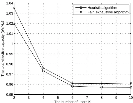
To examine the effect of the number of users on a multi-user multi-carrier system with limited resources, Fig. 9 includes the plots for the total EC value versus the number of users K, for the heuristic algorithm and the fair-exhaustive algorithm. Specifically, the total number of available subcarriers is fixed at N = 10. All users are assumed to have the same circuit-to-noise power ratio Pcr = −10dB, the same delay QoS exponent θ = 0.01, and the same EE requirement factor

χEE = 0.7. When the number of users K increases, the total EC values calculated from the two algorithms decrease and then stabilize when K ≥ 6. This happens because, when K

increases from 2 to 6, the number of served users increases and correspondingly, the number of subcarriers allocated to each served user decreases. Henceforth, the achievable EC for each served user reduces and the total EC value calculated from (7) decreases. WhenK≥6, the number of served users remains the same, due to the limited number of available subcarriers. Hence, the total EC value stays stable when K

becomes greater than 6.

4 6 8 10 12 14 1

1.01 1.02 1.03 1.04 1.05 1.06 1.07 1.08 1.09

The number of subcarriers N

Total effective capacity (b/s/Hz)

Heuristic algorithm Algorithm in [24]

Fig. 10: The total effective capacity versus the number of subcarriersN, for heuristic algorithm and algorithm in [25] .

needs to be minimized. Since in our paper, we have link-layer EE requirement for each user, for the initial subcarrier allocation vector, we will make the elements proportionate to the corresponding users’ EE requirements5_{. The number} of users is K = 4, and all the users are assumed to have the same delay QoS exponent, i.e.,θ= 0.001, and the same EE requirement factor, i.e.,χEE = 0.7. When the number of subcarriers increases, the total EC values calculated from the two algorithms first increase and then gradually stabilize. This indicates that when all users have loose delay QoS require-ments, increasing the number of available subcarriers will not greatly improve the total system EC value. Further, from Fig. 10, it shows that our proposed heuristic algorithm performs better than the algorithm in [25]. Apart from this, the allocation algorithm in [25] also has no guarantee of each user’s link-layer EE requirement, which can be confirmed from Fig. 14. Hence, we can conclude that, to solve the formulated total EC-maximization problem, subject to all users’ EE requirement constraints, our proposed heuristic algorithm is more suitable, because it outperforms the algorithm in [25], and is also simple, fair and close-to-optimal.

Assume that all K users, having the same θ value at

θ= 0.01, and the same circuit-to-noise power ratio value at

Pcr =−10dB, are split into two groups. In group 1, all K1 users are required to have the same χEE, i.e., χEE = 0.1. Meanwhile, the EE requirement factor value χEE for all

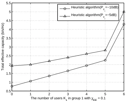
K −K1 users in group 2 is 0.8. This indicates that the users in group 1 have looser EE requirements compared to the users in group 2. Set the total number of users K = 6, and the total number of subcarriersN = 12. Fig. 11 includes the plots for the results of the system total EC versus the number of usersK1 in group 1, for various values of circuit-to-noise power ratioPcr. With fixed Pcr, whenK1 increases from 0 to 6, the total system EC value, in b/s/Hz, gradually increases. This is because when K1 increases, the number of users with χEE = 0.1 increases and correspondingly, the number of users with χEE = 0.8 reduces. We note that for

5_{Hence, we had to tweak the algorithm slightly to be able to provide these} results.

0 1 2 3 4 5 6

0.5 1 1.5 2 2.5 3 3.5 4 4.5 5 5.5

The number of users K₁ in group 1 with χ_EE = 0.1

Total effective capacity (b/s/Hz)

Heuristic algorithm(P

c_r=−10dB)

Heuristic algorithm(P

c_r=−5dB)

Fig. 11: The total effective capacity versus the number of usersK1

in group 1, for various values ofPc_r.

each user, a large χEE value means that the user has a strict requirement on its link-layer EE value and will end up with a relatively small EC value. Therefore, when the number of users withχEE= 0.8reduces, the system can save more resource to benefit the total system EC value, rather than sacrifice the system performance to support the strict EE requirements. When K1 increases from 5 to 6, the number of users with

χEE= 0.8 reduces from 1 to 0 and the total EC value grows dramatically. This is due to the fact that in the check process of heuristic algorithm, the user having current minimum EC value will get the priority, which, in this case, corresponds to the one with χEE = 0.8. Therefore, when K1 = 5, the heuristic algorithm spends many resources on the user with

χEE = 0.8. When K1 = 6, all users have the same loose EE requirements, i.e., χEE= 0.1, therefore, the system resources can be arranged evenly, which results in a great growth in the total EC value. Furthermore, from Fig. 11, we note that whenPcrbecomes larger, the system total EC value increases. Since a bigger value ofPcr for all users will not change their relative difference, and correspondingly, will not change the subcarrier assignment solution, this phenomenon indicates that given a fixed subcarrier assignment, when one user’s circuit power value increases, the system total EC value will increase, as well as its own EC value.

To analyze the impact of the circuit-to-noise power ratio

Pk

cr and the EE requirement factorχ k

EEon thekthuser’s multi-carrier system, Fig. 12 plots the results of the link-layer EE (on the left hand side (LHS) y-Axis, in solid lines) and the optimal tradeoff average power (on the right hand side (RHS) y-Axis, in dash lines) versusPk

cr, for two different values of

χk

EE, consideringNk = 4andθk = 0.01. WhenχkEE is fixed, the link-layer EE value decreases and the optimal average power increases withPk

cr, which confirms the proved Lemma 1. Furthermore, with a fixed value ofPk

cr, whenχ k

EEbecomes larger, the kth _{user’s link-layer EE value increases, but the} optimal average power decreases, which confirms the proposed Lemma 2 in Section III-B.

The plots of EE (on the RHS y-Axis, in dash lines) and EC (on the LHS y-Axis, in solid lines) versus χk

0.1 0.2 0.3 0.4 0.5 0.6 0.7 0.8 0

0.2 0.4 0.6 0.8 1

Circuit−to−noise power ratio

Link−layer energy efficiency (b/J/Hz)

0.1 0.2 0.3 0.4 0.5 0.6 0.7 0.80 2 4 6 8 10

Optimal average power (Watt)

χk EE=0.5

χk EE=0.7

×1/K

l

Fig. 12: Link-layer energy efficiency and the optimal average power versus circuit-to-noise power ratioPk

c_r, for various values ofχ

k

EE.

0 0.2 0.4 0.6 0.8 1

0 1 2 3 4 5 6 7 8 9 10

χk EE

Effective capacity (b/s/Hz)

0 0.2 0.4 0.6 0.8 10

1 2

Link−layer energy efficiency (b/J/Hz)

N

k=1, θk=0.001

N

k=1, θk=0.01

N

k=8, θk=0.001

N_k=8, θ_k=0.01 ×1/K_l

Fig. 13: Effective capacity and link-layer energy efficiency versus

χkEE, for various values ofθk andNk.

different values of delay QoS exponentθk and various values ofNk, are included in Fig. 13. From this figure, we note that with fixed number of subcarriersNk, whenχkEEincreases, EE increases. This confirms the proposed Lemma 2 in Section III-B. Furthermore, with a fixedNk, EC decreases withχkEE. This is due to the fact that the tradeoff system operates in the conflicting region of EE and EC, therefore the EE-increases result from EC-reductions. Moreover, with fixedχk

EEandθk, as the number of subcarriers increases, both EC and EE increase. With fixed Nk, when the delay QoS exponent θk increases from 0.001 to 0.01, both EE and EC decrease. Especially, whenNk= 1, the decreases of EE and EC, as a result of the increase in θk, are significant. However, when Nk is larger, e.g.,Nk = 8, the decreases of EE and EC are minor. This indicates that the multi-carrier communication system is more robust against delay requirements, in comparison with single-carrier communication systems. In other words, when the system QoS requirement becomes more stringent, the multi-carrier system would sacrifice less EE and EC to guarantee the requiredθk.

To further analyze and investigate the effect ofχEEon the

0.1 0.2 0.3 0.4 0.5 0.6 0.7 0.8 0.9 0.5

1 1.5 2 2.5 3 3.5 4 4.5

EE requirement factor χ

EE

Total effective capacity (b/s/Hz)

Heuristic algorithm(θ=0.001) Heuristic algorithm(θ=0.1) Fair−exhaustive algorithm(θ=0.001) Fair−exhaustive algorithm(θ=0.1) Algorithm in [24] (θ=0.001) Algorithm in [24] (θ=0.1)

Fig. 14: The total effective capacity versus EE requirement factor

χEEfor different values ofθin heuristic algorithm, fair-exhaustive

algorithm and algorithm in [25].

0 1 2 3 4 5 6 7 8 9

0.7 0.8 0.9 1 1.1 1.2 1.3 1.4 1.5 1.6 1.7

Per−user maximum available power value scaled by K_l (dB)

Total effective capacity (b/s/Hz)

Heuristic algorithm Fair−exhaustive algorithm all θ =0.001

all θ = 0.1

Fig. 15: The total effective capacity versus maximum power value, for different values ofθ_.

multi-user multi-carrier system, Fig. 14 includes the plots for the total EC value versus EE requirement factor χEE, with two different values of θ, for the heuristic algorithm, the fair-exhaustive algorithm and the algorithm in [25]. Assume that the total number of users K = 4 and the total number of available subcarriers N = 8. Specifically, all K users have the same settings of delay QoS exponentθ, χEE, with

Pcr =−10dB. WhenχEE increases, the total EC value of the multi-user multi-carrier system decreases in the heuristic al-gorithm and the fair-exhaustive alal-gorithm. Furthermore, when

θ = 0.001, the EC curves of the two algorithms are exactly the same. This indicates that for a system withKusers having loose delay requirements, the difference between the total EC values calculated from the two algorithms is very little, even under different subcarrier assignment solutions. Whenθ

10−4 10−3 10−2 10−1 10−5

10−4 10−3 10−2 10−1 100

Delay QoS exponent θ_k (1/bit)

Delay−outage probability

N_k = 8, χk_EE=0.9

N

k = 8, χ k EE=0.8

Fig. 16: Delay-outage probability versus delay QoS exponentθk, for different values ofχEE.

when χEE increases, the total EC value stays stable. This is because, this algorithm proposed in [25] does not guarantee all users’ EE requirements. Therefore, in this case,χEEhas no influence on the total EC value.

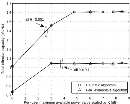
Considering that the value of the maximum available power for each user can influence the optimal results, we include Fig. 15 to show the performance of the heuristic algorithm and the fair-exhaustive algorithm, when the maximum available power value varies. The total number of subcarriers is fixed atN = 6, and the number of users isK = 4. All users are assumed to have the same settings for χEE, i.e., χEE = 0.5, and the same circuit-to-noise power ratio, i.e.,Pcr =−10dB. In addition, two different scenarios of delay QoS exponent vector θ are included in Fig. 15, i.e., all elements in θ are either 0.001 or 0.1. Firstly, we note that in both scenarios, the calculated final EC values from the two algorithms are close, only with very little difference which makes the two curves difficult to distinguish. This confirms that the proposed heuristic algorithm indeed guarantees a close-to-optimal per-formance. Furthermore, when all users have more stringent delay QoS requirements, the total EC value reduces, which means that the value of EC needs to be sacrificed in this situation. More importantly, from Fig. 15, we can notice that for a fixedθ, the curves first increase, and then stabilize. This is because when the maximum available power value is too small to support the proposed optimal power value, the system has to operate atPmax. Therefore, the final calculated EC value is smaller in this case, since it is obtained atPmax, rather than at the optimal power value. On the other hand, when the value of

Pmax becomes larger than the proposed optimal power value, then the system will operate at the optimal average power, which gives the maximum EC value, under each user’s EE constraint. To find detailed analysis, please refer to Section III-B.

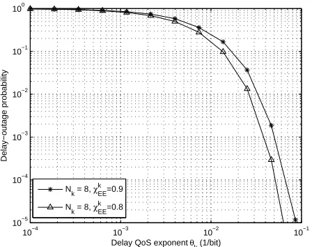
Fig. 16 plots the delay-outage probability for the kth _user,

Pout

delay, versus delay QoS exponentθk, for various values ofχkEE with a maximum tolerable delay thresholdDmax= 200and the circuit-to-noise power ratioPk

cr=−10dB. This figure reveals that for loose delay-constrained situations, e.g.,θk = 10−4,

the achievable Pout

delay values stay the same with different

χk

EE values. When the delay requirement is more stringent, e.g.,θk = 10−2, smaller χkEE ends up with less delay-outage probability. This happens because smaller χk

EE value means more sacrifices of EE from its maximum value, and in turn, results in more increases in its EC value. Therefore, the probability that the buffer length exceeds Dmax decreases, henceforth, the delay-outage probability reduces.

V. CONCLUSIONS

A close-to-optimal subcarrier assignment solution jointed with an optimal power allocation strategy for end users to maximize the system total EC value, subject to all users’ aver-age transmission power limits and link-layer EE constraints in a multi-user multi-carrier uplink network, were proposed and developed in this paper. The traditional exhaustive algorithm was introduced, followed by a fair-exhaustive algorithm, which offers the optimal frequency provisioning solution in a fair manner. To reduce the computational complexity, we proposed a fair heuristic algorithm, which offers close-to-optimal solu-tions, and has a low complexity linearly relating to the size of the problem. Given the subcarrier allocation matrix, the power-constrained EC maximization problem in the single-user multi-carrier system, under each single-user’s individual link-layer requirement level, was solved. To thoroughly analyze the tradeoff problem, the effects of the circuit power and the EE requirement factor were proved and investigated. Simulation results confirmed our design intentions, and further revealed that when there is a link-layer EE constraint, each user’s tradeoff EC value may not monotonically decrease with its delay QoS provisioning, and the tradeoff EC value obtained with less subcarriers may be higher than the one achieved with more subcarriers.

APPENDIXA: PROOF OFLEMMA1

Assume that the calculated tradeoff average power value for thekth _{user, obtained with a circuit power valueP}k

c,1, can

be denoted as P∗

k,1. Meanwhile, when the allocated number

of subcarriers is N, the maximum achievable EE value, i.e.,

ηmax,1k,N = EE k

Nk=N

Pk

c=Pck,1 Pk=Pk

∗

EE,1

, achieves at Pk∗

EE,1. If the kth user has

a higher circuit power, i.e, Pk

c,2 = Pck,1+ ∆Pck, ∆Pck >0,

the corresponding average power values which satisfy the EE requirement equality (20) and ηk,N_max,2 can be written as P∗

k,2

and Pk∗

EE,2, respectively. From (20), we have the following equations:

EEk

Pck=Pck,1 Pk=Pk,∗1

=χk

EE×EEk

Nk=N

Pk

c=Pck,1 Pk=Pk

∗

EE,1

, (22a)

EEk_Pk

c=Pck,2 Pk=Pk,∗2

=χk EE×EE

k

Nk=N

Pk

c=Pck,2 Pk=Pk

∗

EE,2

. (22b)

In order to investigate the influence of circuit powerPk

c on

the tradeoff EE value, we start from analyzing the effect ofPk

c