American Society of
Mechanical Engineers
ASME Accepted Manuscript Repository
Institutional Repository Cover Sheet
Michele Sergio Campobasso
First Last
ASME Paper Title: WIND TURBINE DESIGN OPTIMIZATION UNDER ENVIRONMENTAL UNCERTAINTY
Authors: M. Caboni, M.S. Campobasso, E. Minisci
ASME Journal Title: Journal of Engineering for Gas Turbines and Power
Volume/Issue 138(8) Date of Publication (VOR* Online) 15 March 2016
ASME Digital Collection URL:
http://gasturbinespower.asmedigitalcollection.asme.org/article.aspx?articleid=2491260&resultClick=1
DOI: 10.1115/1.4032665
ASME ©; CC-BY distribution license
PAPER GTP-15-1576
WIND TURBINE DESIGN OPTIMIZATION UNDER ENVIRONMENTAL UNCERTAINTY
Marco Caboni∗ School of Engineering
University of Glasgow
Glasgow, G12 8QQ, United Kingdom
M. Sergio Campobasso†
Department of Engineering
Lancaster University
Lancaster, LA1 4YR, United Kingdom
Edmondo Minisci Department of Mechanical and
Aerospace Engineering
University of Strathclyde
Glasgow, G1 1XJ, United Kingdom
ABSTRACT
Wind turbine design optimization is typically performed considering a given wind distribution. However, turbines so
de-signed often end up being used at sites characterized by different wind distributions, and this results in significant
perfor-mance penalties. This paper presents a probabilistic integrated multidisciplinary approach to the design optimization of
multi-megawatt wind turbines accounting for the stochastic variability of the mean wind speed. The presented technology is applied
to the design of a 5 MW rotor for use at sites of wind power class from 3 to 7, where the mean wind speed at 50 m above the
ground ranges from 6.4 to 11.9 m/s. Assuming the mean wind speed to vary stochastically in such range, the rotor design is
optimized by minimizing mean and standard deviation of the levelized cost of energy. Airfoil shapes, spanwise distributions
of blade chord and twist, blade internal structural layup and rotor speed are optimized concurrently, subject to structural
and aeroelastic constraints. The probabilistically designed turbine achieves a more favorable probabilistic performance than
the initial baseline turbine. The presented probabilistic design framework is portable and modular in that any of its analysis
modules can be replaced with counterparts of user-selected fidelity.
∗Researcher. Energy research Centre of the Netherlands. ECN, P.O. Box 1, 1755 ZG Petten, the Netherlands. Email: [email protected].
NOMENCLATURE
AoA Angle of Attack.
AEP Net annual energy production. BEM Blade-element momentum. BLC Bottom lease cost.
CD Drag coefficient.
CL Lift coefficient.
D Lifetime damage. DLC Design load case.
EWM Extreme wind speed model. FRC Fixed charge rate.
HAWT Horizontal axis wind turbine. ICC Initial capital cost.
IEC International Electrotechnical Commission.
K Torque control parameter in region 2. LCOE Levelized cost of energy.
LRC Levelized replacement/overhaul cost. MDO Multidisciplinary design optimization.
N Number of blades.
NTM Normal turbulence model.
O&M Levelized operations and maintenance cost. PPI Producer Price Index.
R Buckling parameter.
R Rotor radius.
RDO Robust design optimization.
T Generator torque.
W Blade weight.
ccc Array of constraints.
c Chord length.
f Blade first natural frequency.
s Thickness parameter.
u Wind speed. ¯
u Expectation of wind speed distribution.
xxx Array of design variables.
δ Out-of-plane tip deflection.
ϑ Section twist angle.
λ Tip-speed ratio.
µLCOE Expectation of LCOE . ω Rotor angular speed.
σ Normal stress.
σLCOE Standard deviation of LCOE.
INTRODUCTION
The design of wind turbines is a multidisciplinary process, integrating aerodynamic, structural, environmental, manufacturing, transportability and cost considerations. The use of multidisciplinary design optimization (MDO) [1] constitutes a promising way to enhance the profitability of wind turbines. In recent years, several studies have been devoted to the MDO of wind turbines, encompassing a wide variety of approaches and techniques [2–10].
Reduced Quadrature approach [14], and a two-stage multi-objective evolution-based optimization strategy was used. Caboni et al. [15] generalized the probabilistic design approach of [13] by including also the airfoil geometry in the probabilistic design environment, and applied this technology to maximize the expectation and minimize the standard deviation of the annual energy production of a multi-megawatt rotor subject to geometric uncertainty. Using a gradient-based optimizer, Ning et al. [16] designed a wind turbine rotor to be used across diverse sites characterized by a different mean of the wind distribution. Subject to a set of structural constraints, the expecta-tion of the levelized cost of energy (LCOE) was minimized by adopting optimal blade chord, twist, and spar cap thickness distribuexpecta-tions, and rotor speed, diameter and rated power.
To ensure structural integrity, wind turbines must satisfy an extensive set of structural requirements, relating to material ultimate and fatigue strength, deflections and structural stability. In the literature, however, wind turbine design optimization is generally subject only to a limited number of structural constraints, neglecting criteria the violation of which may result in structural failure. Ashuri et al. [17] defined the minimum number of structural constraints that should be considered to obtain a practical design. Using a gradient-based algorithm, these authors optimized the rotor and tower of a wind turbine for minimum LCOE. Blade design variables encompassed chord and twist distribution, blade length, rated rotor speed and structural thicknesses along the span.
Another important limitation affecting most reported HAWT MDO studies is that airfoil design is not handled within the rotor optimization, although such inclusion plays a fundamental role in both aerodynamic and structural turbine performance [2]. This issue was recently investigated by Bottasso et al. [18], who optimized concurrently the airfoil shapes and the chord and twist spanwise distributions of a 2 MW wind turbine blade subject to a set of structural constraints. A gradient-based algorithm was used to solve the optimization problem.
The paper starts by presenting the aerodynamic, aeroelastic, structural and cost analysis models. It then defines the rotor geometry parametrization, and it illustrates its use for the parametrization of the reference 5 MW HAWT rotor. This is followed by the definition of the optimization problem, including the design variables, the objective function and the constraints. Thereafter, the result of the probabilistic design optimization and the reference turbine are compared, whereas the main conclusions of the study and future work are summarized in the concluding section.
MULTIDISCIPLINARY ANALYSIS FRAMEWORK
The multidisciplinary analysis framework for the integrated rotor design is made up of several modules linked together in a MAT-LAB environment. Such framework is based on an aero-servo-elastic model that analyzes the aerodynamic, aeroelastic and structural characteristics of the rotor, and a cost model used to assess the economical performance of each rotor. All components of the multidis-ciplinary analysis system are briefly described below.
Aerodynamics. Rotor aerodynamic and aeroelastic analyses require airfoil aerodynamic loads. Two-dimensional (2D) airfoil lift and drag coefficients are calculated using the airfoil analysis code XFOIL [20]. In this code, transition from laminar to turbulent flow along the airfoil is modeled with the eNmethod. For all optimizations reported below, the turbulence intensity-related NCRIT parameter was kept at the default value of 9. Unfortunately, XFOIL is unsuitable for the solution of stalled flows. Thus, in this study the code was used for a relatively limited range of the angle of attack (AoA), namely from an angle close to the zero-lift AoA to an angle slightly higher than the maximum lift coefficient AoA, assumed to indicate the onset of stall. In these analyses, the Reynolds number varied from 2·106to 14·106. The three-dimensional (3D) aerodynamic analysis of HAWT rotor flows requires lift and drag data of the blade
airfoils over a wider range than that considered by the XFOIL simulations. Airfoil data over a wider AoA range were obtained using AERODAS, an empirically-derived model for airfoil force calculations [21]. AERODAS enables the calculation of near- and post-stall lift and drag airfoil characteristics using as input a limited amount of pre-stall 2D aerodynamic data of the airfoil being considered. In this study, AERODAS polars for AoA ranging from -180 to 180 deg were computed using the zero-lift AoA, the maximum lift and drag coefficients, the AoA at maximum lift and drag, the slope of the linear part of the lift curve, and the minimum drag coefficient, and all these input data were extracted by the XFOIL analyses. An interesting feature of the AERODAS equations is that they correct the infinite-length airfoil (2D) data to account for the effect of finite blade aspect ratios, thus taking into account tip and root losses.
the AoA of maximum lift [24]. Unfortunately, run-times of Navier-Stokes codes, even in 2D simulations, are still excessive for their use in design optimizations requiring hundreds or thousands of rotor analyses, and RFOIL is not an open-source tool and could thus not be used in this study. The use of AERODAS for near- and post-stall airfoil data prediction also introduces some uncertainty in the aerodynamic analysis. The AERODAS model was built with an empirical approach based on the trends of experimental data of several low-speed airfoils. These trends were modeled by a set of algebraic equations providing the best fit of the experimental data. The AERODAS analysis of wind turbine airfoils featuring aerodynamic characteristics significantly different from those of the airfoils used to build the model may yield insufficiently accurate results.
Due to the uncertainty associated with the use of XFOIL and AERODAS, some features of the probabilistic optimal design reported below may require further verification. The main objective of the probabilistic turbine design optimization exercise presented herein, however, is to explore the potential of robust design optimization for improving general integrated multidisciplinary HAWT design technologies, rather than proposing a ready-for-installation design.
Aeroelasticity and stress analysis. The aeroelastic simulations of the turbine rotor are performed by means of FAST [25], which is linked to an external library defining the control system described below. For each wind speed and rotor geometry, FAST is used to predict the rotor speed and power, as well as blade deformations and ultimate and fatigue loads. Rotor aerodynamics is analyzed with AeroDyn [26], a library implementing the blade-element momentum (BEM) theory [27] and several corrections, including the Prandtl’s correction to account for tip and hub losses, and the correction accounting for axial induction factors exceeding the maximum theoretical limit of 0.5. In the analyses below, however, Prandtl’s correction was disabled because the 2D airfoil data are already corrected to account for finite aspect ratio effects in AERODAS. FAST employs a linear modal representation to characterize blade flexibility. Blade modes depend on rotor speed, blade geometry and span-variant structural properties. Blade span-variant structural properties and blade modes are computed by means of the structural analysis code Co-Blade [28] and the preprocessor BModes [29], respectively. Making use of a blend of classical lamination theory, the Euler-Bernoulli theory and shear flow theory applied to composite beams, Co-Blade predicts both the composite blade structural properties, and its deformation and material stress fields. In this study, deformations and material stresses have been determined by Co-Blade using the aerodynamic loads calculated by AeroDyn.
Cost model. LCOE is the figure of merit used to assess the economical performance of each design and the LCOE model adopted herein is based on the DOE/NREL scaling model [30]. According to such model, the LCOE of an offshore HAWT is given by:
LCOE=(FRC·ICC) +BLC+O&M+LRC
where FRC is the fixed charge rate, ICC is the initial capital cost, BLC is the bottom lease cost, O&M is the levelized operations and maintenance cost, LRC is the levelized replacement/overhaul cost, and AEP is the net annual energy production. Although only the rotor design is considered in the optimization study of this paper, the LCOE of each design refers to the cost of the whole turbine, including drive train, nacelle, tower and foundations. This is accomplished by including in ICC the cost of all turbine components, which results in this variable being the sum of a term proportional to the blade mass varying with the particular rotor configuration, and a constant term, referring to the overall costs of all other components.
The costs of the turbine components indicated in the DOE/NREL scaling model were based on 2002 dollars. Therefore, these costs needed to be updated to account for the year-over-year change in products, material and labor costs. Cost escalation was based on the Producer Price Index (PPI). The PPI, maintained and updated on a monthly basis by the U.S. Department of Labor, Bureau of Labor Statistics, tracks the price change of a wide range of product (or commodity) categories. Commodity escalation factors were determined by using the PPI categories provided by the DOE/NREL scaling model for each turbine component.
DESIGN SPACE AND REFERENCE TURBINE
The airfoil schedule for each rotor blade considered in the optimization process is defined by the geometry of 3 airfoils, namely that at 16.67% blade length (root airfoil), 50% blade length (midspan airfoil) and 100% blade length (tip airfoil). An example of root, midspan and tip airfoil geometry is reported in Fig. 1. The geometry of the airfoils between the root and midspan radii, and the midspan and tip radii is obtained with linear interpolations. As reported below, the geometry of the interpolated airfoils is part of the input of Co-Blade. The geometry of the three base airfoils is parametrized by means of a composite Bezier curve based on 14 points, and made up of two 3rd-order Bezier curves and two 4th-order Bezier curves. The parametrization is illustrated considering the root airfoil reported in Fig. 1. The rear part of the airfoil upper side is based on pointsp1,p2,p3,p4, and is defined by a 3rd order Bezier curve; the front part
of the upper side is based on pointsp4,p5,p6,p7,p8, and is defined by a 4th order Bezier curve; the front part of the lower side is based
on points p8,p9,p10,p11,p12, and is defined by a 4th order Bezier curve; the rear part of the lower side is based on pointsp12,p13,
p14,p1, and defined by a 3rd order Bezier curve. The junction pointp1has only position continuity (C0), whereas position, tangent (C1)
and curvature continuity (C2) is enforced at the junction points p4,p8andp12. In the optimization process, pointsp4,p5, p6, p7,p11
andp12were actively controlled in both x- and y-directions, and this corresponds to 12 degrees of freedom. The leading edge position
(pointp8) and the trailing edge position (pointp1) are fixed at(x=0,y=0)and(x=1,y=0), respectively. Once the position of points
p4,p5,p6,p7,p11andp12is assigned, the coordinates of pointsp2,p3,p9,p10,p13andp14are determined by enforcingC0,C1andC2
continuity at the junctionsp4,p8andp12. Thus, each of the 3 base airfoils is described by 12 independent variables, and therefore 36
design variables, labeledxi, i=1,36, are used to define the blade airfoils from root to tip.
0 0.2 0.4 0.6 0.8 1 1.2 −0.4 −0.3 −0.2 −0.1 0 0.1 0.2 0.3 0.4 x/c y/c p8
p 7
p6 p5 p4
[image:9.612.193.416.134.273.2]p9 p 10 p11 p 12 p3 p2 p 1 p13 p 14 root midspan tip
FIGURE 1. PARAMETRIZATION OF ROOT, MIDSPAN AND TIP AIRFOILS. EACH AIRFOIL IS DEFINED BY A COMPOSITE BEZIER CURVE BASED ON 14 POINTS, HERE SHOWN ONLY FOR THE ROOT AIRFOIL. HORIZONTAL AND VERTICAL ARROWS DENOTE THE ACTUAL DEGREES OF FREEDOM.
0 0.2 0.4 0.6 0.8 1 0 1 2 3 4 5 6 r [−] c [m] c
1 c 2 c3 c4 c5
0 0.2 0.4 0.6 0.8 1 −2 0 2 4 6 8 10 12 14 16 r [−] ϑ [deg] ϑ1 ϑ2 ϑ3 ϑ4
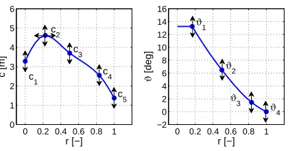
FIGURE 2. PARAMETRIZATION OF CHORD PROFILE (LEFT SUBPLOT) AND TWIST PROFILE (RIGHT SUBPLOT). THE CHORD PRO-FILE IS DEFINED BY A CUBIC SPLINE BASED ON 5 POINTS, AND THE TWIST PROPRO-FILE IS DEFINED BY A CUBIC SPLINE BASED ON 4 POINTS. HORIZONTAL AND VERTICAL ARROWS DENOTE THE ACTUAL DEGREES OF FREEDOM.
the chord profile and 4 control points for the twist distribution. The control points of the chord profilec1,c3,c4,c5are fixed at 0%, 50%,
83.33% and 100% the blade span, respectively, whereas pointc2is actively controlled also in the radial direction. Hence, 6 independent
design variables, labeledxi, i=37,42, are used to define the chord profile. The active degrees of freedom for the parametrization of
the chord profile are reported in the left subplot of Fig. 2. The control points of the twist profileϑi,i=1,4 are fixed at 16.67%, 50%,
83.33% and 100% blade span, respectively. Hence, 4 independent design variables, labeledxi, i=43,46, are used to define the twist
profile. The active degrees of freedom for the parametrization of the twist profile are reported in the right subplot of Fig. 2.
[image:9.612.201.411.361.471.2]controlling the blade internal structure and is labeledx47.
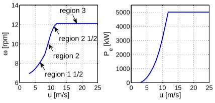
Turbine power control is accomplished by means of variable-speed and variable-pitch. The design specifications include that the cut-in and cut-out wind speeds are 3.0 and 25.0 m/s respectively, and the rated electrical power is 5 MW. A typical rotor speed curve is reported in the left subplot of Fig. 3. This curve consists of 5 regions denoted respectively by 1 (not shown), 11/2, 2, 21/2and 3. Region
1 is a region below the cut-in wind speed in which no power is generated, instead the wind is used to accelerate the rotor. In region 2, the power capture is optimized by making the rotor work at a constant optimal tip-speed ratio, allowing it to operate at the peak power coefficient. The tip-speed ratioλ is:
λ=ωR
u
whereω is the rotor angular speed, Ris the rotor radius anduis the wind speed. In region 3, the generator power is kept constant by varying the blade pitch. Region 11/2is a transition region between regions 1 and 2, while region 21/2is a transition region between regions 2 and 3. Region 21/2is needed to limit the tip speed (and therefore noise emissions) at rated power and above the rated wind
speed. Throughout region 2 the generator torqueT is controlled to maintain a constantλ. In this region, the control of the rotor speed is accomplished by varyingT proportionally to the square of the rotor speed, that is by imposing:
T=Kω2 (2)
whereKis a control variable discussed below. A typical power curve corresponding to the control strategy described above is reported in the right subplot of Fig. 3. In the design optimization reported below, the tip-speed ratio in region 2 is controlled by means of the torque control parameterKin Eq. 2, which is therefore treated as a design variable, and is labeledx48.
0 5 10 15 20 25 0
1000 2000 3000 4000 5000
u [m/s] Pe
[kW]
0 5 10 15 20 25 6
8 10 12 14
u [m/s]
ω
[rpm]
region 1 1/2 region 3
[image:11.612.200.414.153.256.2]region 2 region 2 1/2
FIGURE 3. ROTOR SPEED (LEFT SUBPLOT) AND ELECTRIC POWER (RIGHT SUBPLOT) AGAINST WIND SPEED. LEFT SUBPLOT REPORTS DIFFERENT CONTROL REGIONS.
starting the design optimization, the geometry of the blade of the NREL 5 MW turbine given in [19] as well as its internal structural layup and rotor speed have been redefined using the parametrization defined above. This has been done both to build a convenient initial solution for the optimization, and to determine the performance of the reference turbine using the same modeling set-up of the multidisciplinary analysis used to redesign the turbine and determine the performance of the new design. Parametrizing the external geometry of the reference turbine has involved finding the best geometric fit for the root, midspan and tip airfoils, which are the DU 99-W-405, DU 91-W2-250 NACA 64-618 airfoils, respectively. Parametrization control points of the reference turbine’s chord and twist distributions have been determined as the best fit to the NREL offshore 5-MW baseline wind turbine’s chord and twist distributions. In order to make a fair comparison between the optimized and the reference turbines, both the thickness parametersand the torque control parameterKof the reference turbine have been optimized for minimum LCOE subject to the structural constraints described below for a mean wind speed of 10.0 m/s. The rotor speed curve and the power curve depicted respectively in the left and right subplots of Fig. 3 refer to the modified reference turbine. Additional information on the design specifications and turbine definition of the original NREL 5 MW turbine is available in [19].
DESIGN OPTIMIZATION
Objective function. RDO aims at finding a design with the best possible performance and minimal sensitivity to design, control and/or environmental uncertainty. RDO problems are generally formulated and solved in terms of multiple objective functions, typically involving the mean and standard deviation of one or more deterministic objective functions. The performance parameter considered in this study is LCOE, the definition of which is provided by Eq. (1), and the goal of the RDO exercise reported below is to minimize both the expectation and the standard deviation of LCOE considering the uncertainty affecting the mean wind speed. This is a multi-objective design optimization problem, and it can be solved using either ad-hoc bi-multi-objective optimization approaches [33], including evolution-based algorithms [13], or single-objective approaches [33]. Optimizing the mean and minimizing the standard deviation are often conflicting targets, underlying the existence of a Pareto set of optimal solutions. One of the simplest single-objective approaches to robust optimization is the weighted sum method, whereby a single objective function is obtained by considering a weighted average of mean and standard deviation of the performance parameter of interest. When a Pareto front exists, each of its points could be determined by varying the weights and solving a new optimization problem. Although rather simple to implement and often quite robust, this approach to the calculation of the entire Pareto front suffers from some limitations, including its inadequacy to determine non-convex regions of the front [34].
Using the weighted average method, the objective function to be minimized in the considered HAWT design problem is:
f(xxx,u¯) =α
µLCOE(xxx,u¯)
µ∗
LCOE
+ (1−α)
σLCOE(xxx,u¯)
σ∗
LCOE
(3)
wherexxxis the array of 48 design variables defined in the preceding section,µLCOEandσLCOEare respectively the mean and the standard
deviation of LCOE of the current HAWT design, and µ∗
LCOE andσLCOE∗ denote the values of these two parameters for the reference
turbine. These two values are thus used to normalize the probabilistic estimate of LCOE of all considered HAWT rotor designs. The values ofµLCOEandσLCOEfor each HAWT are calculated by applying the definition of these variables to the set of mean wind speeds
obtained by subdividing the considered interval [7.0 m/s, 13.0 m/s] into 100 equally spaced intervals.
The constantsα and(1−α)define respectively the weight assigned toµLCOE andσLCOE. In this work, equal weights are given
toµLCOEandσLCOE, i.e. α=0.5. Thus, it has not been attempted to determine the entire Pareto front of optimal solutions. However,
Constraints. The IEC 61400-3 standard specifies an essential set of design requirements to ensure the structural integrity of offshore wind turbines. This standard prescribes a number of design load cases (DLCs) which define design situations, wind conditions and types of analysis to be considered during the structural design of wind turbine components. Design situations include normal, fault, and parked operating conditions, while wind conditions, divided into normal and extreme, depend on the wind turbine class. Wind turbine classes are defined in terms of wind speed and turbulence parameters of the intended installation site. The types of analysis prescribed by the standard are divided into analysis of ultimate loads and analysis of fatigue loads. Ultimate load analysis refers to the assessment of material strength, blade tip deflection and structural stability, while fatigue load analysis concerns fatigue strength. The standard also determines safety factors to be applied to ultimate and fatigue loads. In addition, the IEC 61400-3 standard specifies marine conditions (waves, sea currents, water level, etc.) which should be included in the design of offshore wind turbines. In this work, however, marine conditions were not considered. A few representative DLCs are taken into account in the present study, namely those denoted by 1.1, 1.2 and 6.1. A turbine class IB(defining a site reference wind speed of 50.0 m/s, and medium turbulence characteristics)
has been selected. For normal operating conditions, the DLCs 1.1 and 1.2 involve the analysis of ultimate and fatigue loads, respectively, using the normal turbulence model (NTM) to define wind conditions. The DLC 6.1 considers instead the analysis of ultimate loads in parked conditions using the extreme wind speed model (EWM) for wind conditions. The parked conditions considered by the DLC 6.1 are achieved by pitching the blades towards feather.
As recommended by the standard, loads were estimated by 6 10-minute stochastic simulations for each mean wind speed considered. These 6 mean wind speeds are chosen between cut-in and cut out speeds for the NTM, while for the EWM the mean of an extreme wind speed with a recurrence period of 50 years is considered. For DLCs 1.1 and 1.2, the wind speed distributions were defined by 11 bins. Each bin had a width of 2.0 m/s, and the mean values of the bins were 4.0, 6.0, 8.0, 10.0, 12.0, 14.0, 16.0, 18.0, 20.0, 22.0 and 24.0 m/s. For DLC 6.1, load calculations were performed for the extreme wind speed of 50.0 m/s with a recurrence period of 50 years. TurbSim [35] was used to create the turbulent wind files for all the DLCs considered. For each mean wind speed, turbulent wind files were generated using 6 different random seeds. With this configuration, 66 10-minute simulations were carried out for the DLCs 1.1 and 1.2, and 6 for the DLC 6.1. For DLCs 1.1 and 1.2, ultimate and fatigue loads were evaluated concurrently, using the same turbulent wind files.
For each ultimate load analysis, blade laminate (or panel) tensile stressσT, compressive stressσC, buckling margins and
out-of-plane tip deflectionδ are evaluated by means of Co-Blade. Panel buckling is assessed by means of a nondimensional buckling parameter R depending on the working compressive stresses and the critical buckling stress in the panel being considered. A panel to operates in a buckling-free mode if the parameter R is smaller than 1 [28]. Maximum tensile and compressive stresses and buckling parameter were calculated on the upper and lower surfaces and the webs of the blade at 0%, 14.3%, 34% and 63.3% of the blade length.
histories were processed by means of MLife [36], which computes fatigue cycles for each time-series using rainflow counting, and applies Miner’s rule to estimate the lifetime damageD. For design purposes, fatigue failure is assumed to occur whenDis equal to 1. The relationship between load range and cycles to failure (S-N curve) was modeled by means of a Wh¨oler exponent of 10.
To avoid blade resonance, a constraint on the minimum value of the blade first natural frequency f is also enforced. The constraint imposes that the f be greater than the blade passing frequency, namely:
f >Nω ∗
2π (4)
whereN=3 is the number of rotor blades, andω∗is a user-given value of the rotor angular velocity.
As a surrogate for noise constraint, the maximum rotor speed was set to 12.1 RPM, resulting in a maximum tip speed of 80.0 m/s. Each airfoil was subject to several feasibility tests, aiming to avoid unphysical or unconventional shapes. Airfoils with self-intersecting shapes, with more than 1 change of the curvature sign of the suction side, and with more than 2 changes of the curvature sign of the pressure side were discarded. Airfoil relative thickness and its chordwise locations were also subject to feasibility tests. The acceptable variability ranges of the relative thickness of the root, midspan and tip airfoils were chosen to be [38%, 42%], [23%, 27%] and [16%, 20%] respectively. Moreover, acceptable airfoils also had to achieve their maximum thickness between 20% and 40% of the chord.
Laminate tensile and compressive yield strengths were set to 325 MPa and -325 MPa, respectively. With a safety factor of 1.628, the maximum allowable tensile and compressive stresses were 200 MPa and -200 MPa, respectively. A safety factor of 1.628 was used in the buckling verification, resulting in a maximum allowable buckling parameter R of 0.6. The maximum allowable out-of-plane tip deflection was determined by dividing the total blade clearance in unloaded conditions, equal to 10.23 m, by a safety factor of 1.628. This resulted in a maximum allowable out-of-plane tip deflection of 6.28 m. The lifetime damage threshold of 1 was reduced by a safety factor of 1.43, yielding a maximum allowable lifetime damage of 0.7. A minimum value of 0.666 Hz for the first natural frequency of the blade was determined with Eq. (4) using the value ofω∗corresponding to a rotor speed of 12.1 RPM and adopting a safety factor of
1.1.
It should be noted that all the constraints described above, except those on lifetime damage, are deterministic. This means that they do no depend on the mean of the wind distribution. Conversely, the calculation of the lifetime damage is based on the mean of the selected wind distribution, and therefore the associated constraint is enforced on its mean value.
Solution of the optimization problem. Denoting byccc(xxx,u¯)the set of constraints described above, the robust optimization problem is:
Find:xxx={x1, ...,x48}
to minimize: f(xxx,u¯)
where: ¯u∼U(7.0,13.0)
subject to:c(xxx,u¯)
(5)
where f(xxx,u¯)is defined by Eq. (3). The symbols ¯u∼U(7.0,13.0)indicate that the mean wind speed ¯uis uniformly distributed in the range from 7.0 to 13.0 m/s.
ref. rob.
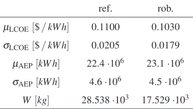
µLCOE[$/kW h] 0.1100 0.1030
σLCOE[$/kW h] 0.0205 0.0179
µAEP[kW h] 22.4·106 23.1·106
σAEP[kW h] 4.6·106 4.5·106
[image:16.612.212.401.128.235.2]W [kg] 28.538·103 17.529·103
TABLE 1. COMPARISON OF THE OVERALL PERFORMANCE OF THE REFERENCE AND ROBUST DESIGNS.µLCOEANDσLCOEARE
MEAN AND STANDARD DEVIATION OF LCOE, RESPECTIVELY;µAEPANDσAEPARE MEAN AND STANDARD DEVIATION OF AEP,
RESPECTIVELY;WIS THE BLADE WEIGHT.
around which the objective function becomes discontinuous and has reduced smoothness.
In this work, the MATLAB pattern search algorithm [37] has been used, and parallelized over 32 processors through the MATLAB distributed computing server tool. This optimizer searches the global minimum of a function by using a set of points, called pattern, which expands or shrinks depending on whether any point within the pattern has a lower objective function value than the current point. As a starting point for the optimization carried out in this study, the reference turbine was used. More detail on the optimizer and the adopted parallelization can be found in the MATLAB documentation [38].
RESULTS AND DISCUSSION
As reported in Tab. 1, the solution of the robust optimization Problem (5) leads to the design of an improved rotor with respect to the reference one, achieving a 6.36% and 12.68% reduction inµLCOEandσLCOE, respectively. The lowerµLCOEis due primarily to the
lower blade weight (- 38.58%), and the enhanced aerodynamic characteristics of the robust rotor, leading to a greater mean of AEP (+ 3.12%). The lowerσLCOEis determined by the 2.17% decrease in the standard deviation of AEP of the robust configuration with respect
to that of the reference turbine.
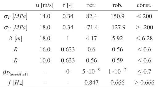
Table 2 compares some structural properties of the reference and the robust turbine blades at selected wind speeds (second column) and radial positions (third column). At a wind speed of 16.0 m/s, the blade of the reference turbine has an active constraint on the maximum allowable buckling stress on the suction side at 63.3% span. The blade of the robust turbine has instead an active constraint on the minimum allowable blade first natural frequency. Table 2 also reports the maximum tensile stressσT and maximum compressive
stressσCacting respectively on the bottom and top surfaces of the two blade designs. One sees that althoughσT andσChave increased
u [m/s] r [-] ref. rob. const.
σT [MPa] 14.0 0.34 82.4 150.9 ≤200 σC[MPa] 18.0 0.34 -71.4 -127.9 ≥-200
δ[m] 18.0 1 4.17 5.92 ≤6.28
R 16.0 0.633 0.6 0.56 ≤0.6
R 10.0 0.633 0.56 0.59 ≤0.6
µD(RootMyc1) - 0 5·10
−9 1·10−2 ≤0.7
[image:17.612.179.435.128.271.2]f [Hz] - - 0.847 0.666 ≥0.666
TABLE 2. COMPARISON OF THE STRUCTURAL CHARACTERISTICS OF THE REFERENCE AND THE ROBUST BLADE DESIGNS AT
SELECTED RADIAL POSITIONSrAND WIND SPEEDSu.σTANDσCDENOTE TENSILE AND THE COMPRESSIVE STRESSES,
RESPEC-TIVELY;δIS THE TIP DEFLECTION; R IS THE BUCKLING PARAMETER;µD(RootMyc1)IS THE MEAN OF THE LIFETIME DAMAGE CAUSED
BY THE OUT-OF-PLANE MOMENT AT THE BLADE ROOT;fIS THE BLADE FIRST NATURAL FREQUENCY AT A ROTOR SPEED OF 12.1
RPM.
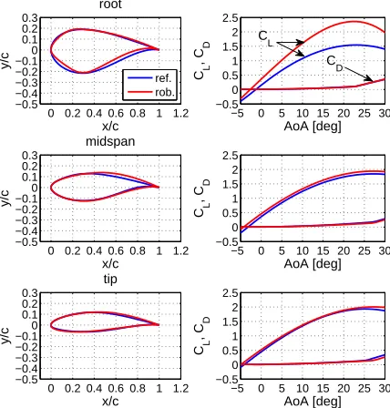
Figure 4 presents the comparison of the airfoils and force coefficients of the reference and robust blade designs. The root, midspan and tip airfoils of the robust design feature a higher lift-to-drag ratio than that of the corresponding reference turbine airfoils. It is observed that, while the maximum airfoil thickness and the chordwise position where such maximum is achieved vary fairly little between corresponding airfoils of the two blade designs, the airfoils of the robust blade are more cambered than those of the reference blade. The camber line, defined as the locus of the points midway between the suction and pressure sides, plays a crucial role in the improvements of the robust airfoils’ aerodynamic performance. Indeed, the larger amount of camber of the robust blade airfoils enables them to achieve a higher lift coefficient. This is particularly evident for the root airfoil, the maximumCLof which is about 50% higher
than that of the reference blade root airfoil. The optimization of the airfoil shapes is also driven by structural considerations. In particular, the midspan airfoil has a lower mean radius of curvature over the aft portion of the suction side with respect to the reference airfoil. This results in an increase of the buckling strength of the blade laminates at a location characterized by a high buckling stress concentration (i.e., over the aft part of the top surface, at around half-span of the blade).
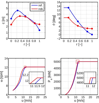
Radial chord and twist profiles of the two designs are reported respectively in the left and right top subplots of Fig. 5. Due to smaller chord lengths of the robust blade design (top left subplot of Fig. 5), this rotor has a lower solidity at most radii, and this occurrence contributes significantly to decrease the blade weight. The blade weight reduction is also a result of the 23.6% decrease of the internal structure thickness parameters(see below). The robust blade design also has less twist than the reference design along the inboard part of the blade and more twist along the outboard part. The consequences of this trend are discussed below. The left and right bottom subplots of Fig. 5 report respectively the rotor speed and the electric powerPeof the two turbines against the wind speed. As expected,
the power extracted by the robust HAWT design is higher than that of the reference turbine in regions 11/2, 2 and 21/2. It is also noted that
0 0.2 0.4 0.6 0.8 1 1.2 −0.5 −0.4 −0.3 −0.2 −0.10 0.1 0.2 0.3 x/c y/c root ref. rob.
−5 0 5 10 15 20 25 30 −0.5 0 0.5 1 1.5 2 2.5 AoA [deg] CL , C D
0 0.2 0.4 0.6 0.8 1 1.2 −0.5 −0.4 −0.3 −0.2 −0.10 0.1 0.2 0.3 x/c y/c midspan
−5 0 5 10 15 20 25 30 −0.5 0 0.5 1 1.5 2 2.5 AoA [deg] CL , C D
0 0.2 0.4 0.6 0.8 1 1.2 −0.5 −0.4 −0.3 −0.2 −0.10 0.1 0.2 0.3 x/c y/c tip
[image:18.612.197.411.140.364.2]−5 0 5 10 15 20 25 30 −0.5 0 0.5 1 1.5 2 2.5 AoA [deg] CL , C D CD CL
FIGURE 4. COMPARISON OF AIRFOIL SHAPES, AND LIFT (CL) AND DRAG (CD) COEFFICIENTS OF THE REFERENCE AND ROBUST
DESIGNS FOR A REYNOLDS NUMBER OF 12·106.
ref. rob.
λ [−] 7.3 8.0
K [N·m/s2] 2.33 1.89
s [−] 1 0.76
TABLE 3. TORQUE CONTROL PARAMETERKIN REGION 2 WITH RESULTING TIP-SPEED RATIO IN PARENTHESES, AND
THICK-NESS PARAMETERsOF THE REFERENCE AND ROBUST DESIGNS.
The tip-speed rationλ and the torque control parameterKof the two turbines in region 2 are provided in Tab. 3, which also reports the thickness parametersof the blades of the two turbines. These results highlight that the robust design features an increment of about 10% of the tip-speed ratio, and a reduction of 24% of the thickness of the internal structure over the reference turbine.
The higher mean of AEP of the robust over the reference turbine is determined by a higher power production of the former turbine in regions 11/2, 2 and 21/2, as highlighted above. This improvement is due to both the reported alterations of the outer blade shape, and a
higher rotational speed. All these alterations have conflicting effects on the net power production, and a discussion on their interactions in regions 11/2, 2 and 21/2is provided below. At the inboard sections, the twist reduction of the robust design visible in the top right
0 0.2 0.4 0.6 0.8 1 0 1 2 3 4 5 6 r [−] c [m] ref. rob.
0 0.2 0.4 0.6 0.8 1 −2 0 2 4 6 8 10 12 14 16 r [−] ϑ [deg]
0 5 10 15 20 25 0 1000 2000 3000 4000 5000 u [m/s] Pe [kW] 11 12 4800 5000 5200
0 5 10 15 20 25 6 8 10 12 14 u [m/s] ω [rpm]
[image:19.612.202.411.145.364.2]11 11.5 12 12 12.2
FIGURE 5. COMPARISON OF CHORD AND TWIST DISTRIBUTIONS (LEFT AND RIGHT TOP SUBPLOTS, RESPECTIVELY), AND RO-TOR SPEED AND ELECTRIC POWER AGAINST WIND SPEED (LEFT AND RIGHT BOTTOM SUBPLOTS, RESPECTIVELY) OF THE REF-ERENCE AND ROBUST DESIGNS.
−2 0 2 4 6 8 −60 −50 −40 −30 −20 −10 0 −14 −12 −10 −8 −6 −4 −2 0 x [m] y [m] z [m] aerodynamic forces weight forces a)
[image:20.612.206.411.125.526.2]−2 0 2 4 6 8 −60 −50 −40 −30 −20 −10 0 −14 −12 −10 −8 −6 −4 −2 0 x [m] y [m] z [m] aerodynamic forces weight forces b)
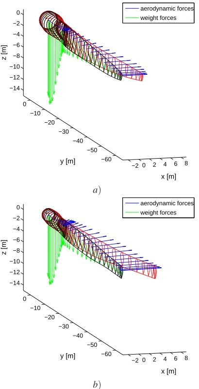
FIGURE 6. DISPLACEMENT AND APPLIED FORCES OFa)THE REFERENCE BLADE DESIGN ANDb)THE ROBUST BLADE DESIGN AT THE 3 O’CLOCK AZIMUTH POSITION FOR A WIND SPEED OF 12.0 M/S AND A ROTOR SPEED OF 12.1 RPM.
The blade displacements and the applied forces of the reference blade design and the robust blade design at the 3 o’clock azimuthal position for a wind speed of 12.0 m/s and a rotor speed of 12.1 RPM are reported in Fig. 6-a and Fig.6-b respectively. Comparing these two sets of results highlightsa)the lighter weight of the inboard part of the robust design, andb)the larger deflections of the robust design resulting from its lower stiffness with respect to the reference blade. The larger deflections are also due to the larger normal component of the aerodynamic force.
a)
[image:21.612.172.464.122.605.2]b)
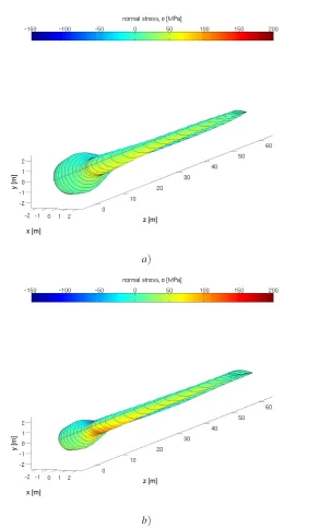
FIGURE 7. LAMINATE NORMAL STRESS OFa)THE REFERENCE BLADE ANDb)THE PROBABILISTICALLY DESIGNED BLADE AT THE 3 O’CLOCK AZIMUTH POSITION FOR A WIND SPEED OF 12.0 M/S AND A ROTOR SPEED OF 12.1 RPM.
REFERENCES REFERENCES
CONCLUSIONS
A novel integrated aero-servo-elastic design framework for the aerostructural design optimization of HAWT rotors has been pre-sented. The developed framework enables the concurrent optimization of the airfoil geometry, the radial profiles of blade chord and twist, the internal structure layup and the rotor speed. Enforcing a comprehensive set of constraints to ensure rotor structural integrity, the design framework has been successfully used to optimize the design of a HAWT rotor subject to the environmental uncertainty associated with the mean value of the wind speed frequency distribution. The robust turbine design achieves a reduction of about 6.4% of the expectation of LCOE, and a reduction of about 12.7% of the standard deviation of this objective function with respect to the deterministic turbine design.
The optimal solutions examined herein may require further verifications due to significant uncertainty affecting the pre-stall air-foil performance predictions of XFOIL, particularly the maximum lift coefficient at the onset of stall, and the corresponding AoA. A significant level of uncertainty is also likely to affect the post-stall airfoil performance prediction of AERODAS, which depends on the pre-stall characteristics predicted by XFOIL and is computed using a good fitting of pre- and post-stall airfoil data referring to a relatively limited number of airfoils. Other sources of uncertainty on aerodynamic performance predictions include the semi-empirical corrections accounting for 3D flow effects in the BEM analysis. The main objective of the probabilistic turbine design optimization exercise presented herein, however, has been to highlight the potential of robust fully integrated multidisciplinary design optimization of improving HAWT design technologies, and this objective has been accomplished.
On the methodology front, future improvements of the developed design framework include the incorporation of higher-fidelity analysis modules, such as transitional Navier-Stokes computational fluid dynamics for pre- and post-stall airfoil aerodynamics, and possibly a full three-dimensional finite element stress analysis code for rotor structural analysis. On the application side, it is envisaged that the developed methodology will be used to carry out the design optimization of utility-scale wind turbine rotors considering other sources of uncertainty, such as those associated with blade manufacturing errors, and the variability of the wind shear associated with the thermodynamic state of the atmospheric boundary layer [39].
ACKNOWLEDGMENT
This project was carried out with support of the wind turbine manufacturer Gaia-Wind, which is hereby acknowledged.
REFERENCES
[1] Martins, J. R. R. A., and Lambe, A. B., 2013. “Multidisciplinary design optimization: A survey of architectures”. AIAA Journal, 51(9), pp. 2049–2075.
REFERENCES REFERENCES
[3] Diveux, T., Sebastian, P., Bernard, D., Puiggali, J. R., and Grandidier, J. Y., 2001. “Horizontal axis wind turbine systems: opti-mization using genetic algorithms”.Wind Energy, 4(4), pp. 151–171.
[4] Fuglsang, P., and Thomsen, K., 2001. “Site-specific design optimization of 1.52.0 MW wind turbines”. Journal of Solar Energy Engineering, Transactions of the ASME, 123(4), pp. 296–303.
[5] Fuglsang, P., Bak, C., Schepers, J. G., Bulder, B., Cockerill, T. T., Claiden, P., Olesen, A., and van Rossen, R., 2002. “Site-specific design optimization of wind turbines”.Wind Energy, 5(4), pp. 261–279.
[6] Kenway, G., and Martins, J. R. R. A., 2008. “Aerostructural shape optimization of wind turbine blades considering site-specific winds”. In 12th AIAA/ISSMO Multidisciplinary Analysis and Optimization Conference, MAO.
[7] Xudong, W., Shen, W. Z., Zhu, W. J., Sørensen, J. N., and Jin, C., 2009. “Shape optimization of wind turbine blades”. Wind Energy, 12(8), pp. 781–803.
[8] Maki, K., Sbragio, R., and Vlahopoulos, N., 2012. “System design of a wind turbine using a multi-level optimization approach”.
Renewable Energy, 43, pp. 101–110.
[9] Bottasso, C. L., Campagnolo, F., and Croce, A., 2012. “Multi-disciplinary constrained optimization of wind turbines”. Multibody System Dynamics, 27(1), pp. 21–53.
[10] Vesel, R. W., and McNamara, J. J., 2014. “Performance enhancement and load reduction of a 5 MW wind turbine blade”.Renewable Energy, 66, pp. 391–401.
[11] Park, G. J., Lee, T. H., Lee, K. H., and Hwang, K. H., 2006. “Robust design: An overview”.AIAA Journal, 44(1).
[12] Petrone, G., de Nicola, C., Quagliarella, D., Witteveen, J., and Iaccarino, G., 2011. “Wind turbine optimization under uncertainty with high performance computing”. In 29th AIAA Applied Aerodynamics Conference 2011.
[13] Campobasso, M. S., Minisci, E., and Caboni, M., 2014. “Aerodynamic design optimization of wind turbine rotors under geometric uncertainty”.Wind Energy. DOI: 10.1002/we.1820.
[14] Padulo, M., Campobasso, M., and Guenov, M., 2011. “A Novel Uncertainty Propagation Method for Robust Aerodynamic Design”.
AIAA Journal, 49(3), pp. 530–543.
[15] Caboni, M., Minisci, E., and Campobasso, M. S., 2014. “Robust aerodynamic design optimization of horizontal axis wind turbine rotors”. InAdvances in Evolutionary and Deterministic Methods for Design, Optimization and Control in Engineering and Sci-ences, D. Greiner, B. Galv´an, J. Periaux, N. Gauger, K. Giannakoglou, and G. Winter, eds., Vol. 36 ofComputational Methods in Applied Sciences. Springer. ISBN 978-3-319-11540-5.
[16] Ning, S. A., Damiani, R., and Moriarty, P. J., 2014. “Objectives and constraints for wind turbine optimization”. Journal of Solar Energy Engineering, Transactions of the ASME, 136(4).
REFERENCES REFERENCES
[18] Bottasso, C. L., Croce, A., Sartori, L., and Grasso, F., 2014. “Free-form design of rotor blades”. Journal of Physics: Conference Series, 524(1).
[19] Jonkman, J., Butterfield, S., Musial, W., and Scott, G., 2009. Definition of a 5-MW Reference Wind Turbine for Offshore System Development. Tech. rep., National Renewable Energy Laboratory, Golden, Colorado, USA. NREL/TP-500-38060.
[20] Drela, M. XFOIL: Subsonic Airfoil Development System. http://web.mit.edu/drela/Public/web/xfoil/, accessed on 30 December 2015.
[21] Spera, D., 2008. Models of Lift and Drag Coefficients of Stalled and Unstalled Airfoils in Wind Turbines and Wind Tunnels. Tech. rep., National Aeronautics and Space Administration, Cleveland, Ohio, USA. NASA/CR2008-215434.
[22] Timmer, W., and van Rooij, R., 2003. “Summary of the Delft University Wind Turbine Dedicated Airfoils”. Journal of Solar Energy Engineering, Transactions of the ASME, 125, pp. 488–496.
[23] Sørensen, N., 2009. “CFD Modelling of Laminar-Turbulent Transition for Airfoils and Rotors Using theγ−Re˜ θ Model”. Wind Energy, 12, pp. 715–733.
[24] Aranake, A., Lakshminarayan, V., and Duraysami, K., 2015. “Computational analysis of shrouded wind turbine configurations using a 3-dimensional RANS solver”.Renewable Energy, 75, pp. 818–832.
[25] Jonkman, J. FAST: An aeroelastic computer-aided engineering (CAE) tool for horizontal axis wind turbines. https://nwtc.nrel.gov/FAST, accessed on 30 December 2015.
[26] Laino, D. J. AeroDyn: A time-domain wind turbine aerodynamics module. https://nwtc.nrel.gov/AeroDyn, accessed on 30 December 2015.
[27] Manwell, J., McGowan, J., and Rogers, A., 2002.Wind Energy Explained. Theory, Design and Application. John Wiley and Sons Ltd.
[28] Sale, D. C. Co-Blade: Software for Analysis and Design of Composite Blades. https://code.google.com/p/co-blade/, accessed on 30 December 2015.
[29] Bir, G. BModes: Software for Computing Rotating Blade Coupled Modes. https://nwtc.nrel.gov/BModes, accessed on 30 Decem-ber 2015.
[30] Fingersh, L., Hand, M., and Laxson, A., 2006. Wind Turbine Design Cost and Scaling Model. Tech. rep., National Renewable Energy Laboratory, Golden, Colorado, USA. NREL/TP-500-40566.
[31] Griffith, D. T., and Ashwill, T. D., 2011. The Sandia 100-meter All-glass Baseline Wind Turbine Blade: SNL100-00. Tech. rep., Sandia National Laboratories, Albuquerque, New Mexico, USA. SAND2011-3779.
[32] IEC 61400-3 Edition 1.0, 2009-02. International Standard. International Electrotechnical Commission.
REFERENCES REFERENCES
[34] Das, I., and Dennis, J., 1997. “A closer look at drawbacks of minimizing weighted sums of objectives for pareto set generation in multicriteria optimization problems”.Structural Optimization, 14(1), pp. 63–69.
[35] Kelley, N., and Jonkman, B. TurbSim: A stochastic, full-field, turbulence simulator primarily for use with InflowWind/AeroDyn-based simulation tools. https://nwtc.nrel.gov/TurbSim, accessed on 30 December 2015.
[36] Hayman, G. MLife: A MATLAB-based Estimator of Fatigue Life. https://nwtc.nrel.gov/MLife, accessed on 30 December 2015. [37] Audet, C., and Dennis, J. E., 2003. “Analysis of Generalized Pattern Searches”. SIAM Journal on Optimization, 13(3), pp. 889–
903.
[38] Mathworks. MATLAB documentation. http://www.mathworks.co.uk/help/matlab/, accessed on 30 December 2015.